A population-based optimization method using Newton fractal

(1)

저작자표시-비영리-변경금지 2.0 대한민국 이용자는 아래의 조건을 따르는 경우에 한하여 자유롭게 l 이 저작물을 복제, 배포, 전송, 전시, 공연 및 방송할 수 있습니다. 다음과 같은 조건을 따라야 합니다: l 귀하는, 이 저작물의 재이용이나 배포의 경우, 이 저작물에 적용된 이용허락조건 을 명확하게 나타내어야 합니다. l 저작권자로부터 별도의 허가를 받으면 이러한 조건들은 적용되지 않습니다. 저작권법에 따른 이용자의 권리는 위의 내용에 의하여 영향을 받지 않습니다. 이것은 이용허락규약(Legal Code)을 이해하기 쉽게 요약한 것입니다. Disclaimer 저작자표시. 귀하는 원저작자를 표시하여야 합니다. 비영리. 귀하는 이 저작물을 영리 목적으로 이용할 수 없습니다. 변경금지. 귀하는 이 저작물을 개작, 변형 또는 가공할 수 없습니다.

(2)

A population-based optimization method

using Newton fractal

Soyeong Jeong

Department of Mathematical Sciences

Graduate School of UNIST

(3)

A population-based optimization method using

Newton fractal

A dissertation

submitted to the Graduate School of UNIST

in partial fulfillment of the

requirements for the degree of

Doctor of Philosophy

(4)

A population-based optimization method using

Newton fractal

Soyeong Jeong

This certifies that the dissertation of Soyeong Jeong is approved.

(5)

Abstract

Metaheuristic is a general procedure to draw an agreement in a group based on the decision making of each individual beyond heuristic. For last decade, there have been many attempts to develop metaheuristic methods based on swarm intelligence to solve global optimization such as particle swarm optimizer, ant colony optimizer, firefly optimizer. These methods are mostly stochastic and independent on specific problems.

Since metaheuristic methods based on swarm intelligence require no central coor-dination (or minimal, if any), they are especially well-applicable to those problems which have distributed or parallel structures. Each individual follows few simple rules, keeping the searching cost at a decent level. Despite its simplicity, the meth-ods often yield a fast approximation in good precision, compared to conventional methods.

Exploration and exploitation are two important features that we need to consider to find a global optimum in a high dimensional domain, especially when prior in-formation is not given. Exploration is to investigate the unknown space without using the information from history to find undiscovered optimum. Exploitation is to trace the neighborhood of the current best to improve it using the information from history. Because these two concepts are at opposite ends of spectrum, the tradeoff significantly affects the performance at the limited cost of search.

In this work, we develop a chaos-based metaheuristic method, Newton Particle Opti-mization(NPO), to solve global optimization problems. The method is based on the Newton method which is a well-established mathematical root-finding procedure. It actively utilizes the chaotic nature of the Newton method to place a proper bal-ance between exploration and exploitation. While most current population-based methods adopt stochastic effects to maximize exploration, they often suffer from weak exploitation. In addition, stochastic methods generally show poor reproducing ability and premature convergence. It has been argued that an alternative approach using chaos may mitigate such disadvantages. The unpredictability of chaos is cor-respondent with the randomness of stochastic methods. Chaos-based methods are deterministic and therefore easy to reproduce the results with less memory. It has been shown that chaos avoids local optimum better than stochastic methods and

(6)

Newton method is deterministic but shows chaotic movements near the roots. It is such complexity that enables the particles to search the space for global optimiza-tion. We initialize the particles position randomly at first and choose the leading particles to attract other particles near them. We can make a polynomial function whose roots are those leading particles, called a guiding function. Then we update the positions of particles using the guiding function by Newton method. Since the roots are not updated by Newton method, the leading particles survive after up-date. For diverse movements of particles, we use modified newton method, which has a coefficient m in the variation of movements for each particle. Efficiency in local search is closely related to the value of m which determines the convergence rate of the Newton method. We can control the balance between exploration and exploitation by choice of leading particles.

It is interesting that selection of excellent particles as leading particles not always re-sults in the best result. Including mediocre particles in the roots of guiding function maintains the diversity of particles in position. Though diversity seems to be in-efficient at first, those particles contribute to the exploration for global search finally. We study the conditions for the convergence of NPO. NPO enjoys the well-established analysis of the Newton method. This contrasts with other nature-inspired algorithms which have often been criticized for lack of rigorous mathematical ground. We com-pare the results of NPO with those of two popular metaheuristic methods, particle swarm optimizer(PSO) and firefly optimizer(FO). Though it has been shown that there are no such algorithms superior to all problems by no free lunch theorem, that is why the researchers are concerned about adaptable global optimizer for specific problems. NPO shows good performance to CEC 2013 competition test problems comparing to PSO and FO.

(7)

(8)

List of Figures

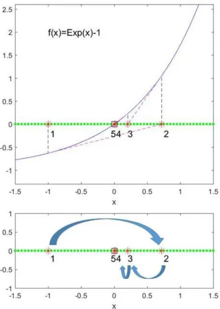
Figure 3-1 An example of dynamics of a particle under a (guiding) function in the 1-dimensional search space: A particle starting from −1 denoted by ‘10 is searching around a root (boxed point) to find a better approximation. The movement is denoted from ‘10 to ‘50.[74] . . . 18

Figure 3-2 Illrustration of the sequences staring from same points. They show dif-ferent behaviors depending on degree coefficientmfor the (guiding) func-tionf(x) =x(x−1)(x−2)[74] . . . 19

Figure 3-3 The basin of attraction of Newton Method shows the Newton fractal. This is an example of Julia sets associated to the Newton method for

f(z) = (z−p₁)(z−p2)· · ·(z−p5). The positions of pi are denoted by

white circles. Each different color region stands for a set of points that converge to the same root by Newton method. Under the same (guiding) function it shows varied fractality depending on degree coefficientm.[74] 21

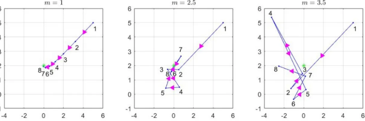
Figure 3-4 Three Newton paths with different degree coefficient m: They are ini-tiated from the same point (5,5). The guiding function is f(z) =

z(z−2i)(z+ 1−i).[74] . . . 21

Figure 3-5 Newton paths generated from slightly different initial points near (3,3) (marked with a black circle): both eventually joins again at the target point (2,−1) (marked with a black square)[74]. . . 22

Figure 3-6 The distribution of particles’ distance from a leading particle(after 50 times of iterations) follows the power law. All particles are initially located on the unit ball centered at the position of a leading particle. The straight lines are the least squares fitting line for log-log scale depending onm. . . 23

(11)

LIST OF FIGURES

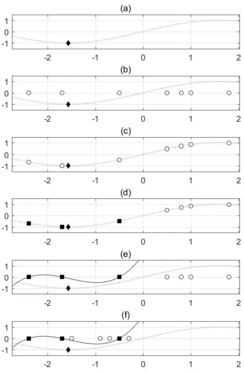
Figure 4-1 NPO Algorithm. (a)A dotted line is represented the hidden fitness func-tion and the global optimum labeled by diamond shape should be found. (b)Distribute the particles in uniformly random manner. These parti-cles are candidate solution and marked by white circle. (c)Evaluate the fitness of the particles. (d)Choose the top 3 best fitters as leading parti-cles. Leading particles are marked with black square label. (e)Make the guiding function with leading particles. (f)Update the other particle’s positions near the best fitter by applying Newton method with guiding

function. Then repeat from (c) until it satisfies the stopping criterion. . 27

Figure 4-2 Performance according tommax. The parameter settings are 200 parti-cles with 4 leading partiparti-cles for rosenbrock function.[74] . . . 33

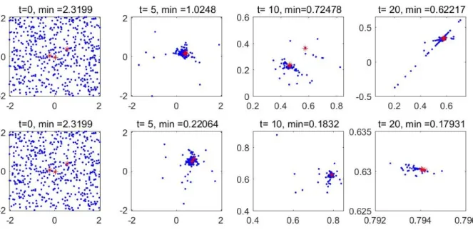
Figure 5-1 A nullcline of a factored guiding function in 2-dimensional space as (4.1.2). 35 Figure 5-2 The distribution of particles using a biased guiding function(above) and a proposed guiding function(below), with same initial condition for the position of particles and degree coefficient m. t counters the iteration step for NPO. mindenotes temporal best. . . 37

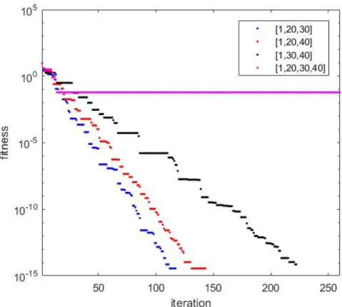
Figure 5-3 The number of leading particles is important. Label denotes the ranking of leading particles among 100 particles. It shows the results ofn= 3 is better than that ofn= 4. . . 38

Figure 5-4 Choice of leading particles affects the result: the above adopts top 5 rank performers out of 100 particles as leading particles. The below uses four best fitters and one 40th rank fitter. The blue and red dots indicate the cost values of ordinary and leading particles, respectively.[74] . . . 39

Figure 6-1 Test functions which have no local minima. . . 44

Figure 6-2 Test functions which have several local minima. . . 45

Figure 6-3 Test functions which have many local minima. . . 46

(12)

List of Tables

Table 6-1 Test Functions[42]. Each minimum of the functions is 0. . . 43

Table 6-2 Benchmark for NPO, PSO, FO: tested with 10-dimensional functions in CEC 2013 competition[74] . . . 49

Table 6-3 Performance comparison of NPO, PSO, and FO in the mean ranking[74] . 50

Table 6-4 Benchmark for NPO, PSO, FO: tested with 30-dimensional functions in CEC 2013 competition . . . 51

(13)

1

Introduction

1.1 Overview

Groups have different characteristics from each individual. Albeit it is insignificant that a taxi driver has a day off, it is significant that taxi drivers have a day off because it is a strike to express their opinion. To settle some big problems, we gather and exchange ideas. Even though feeble organisms such as ants, birds, fishes in nature, they also go around into a group to achieve their goal. It is surprising that they solve the problem effectively pretending to be an intelligent organism. Swarm intelligence emerges in a scale of groups from nature.

Swarm intelligence has been discussed for last two decades. It is closely related with self-organization, decentralized system, dynamical networks, artificial intelligence, etc. Since the swarm intelligence is not a central-control system, it is adaptable to distributed problem-solving. Their decision making process is a natural selection. Natural selection does not mean that na-ture selects the fittest but that the decision is made naturally from multi-agents’ behavior. This kind of decision process is ideal and reasonable for the equality and fairness of members. Each individual follows some simple rules but their actions result in a powerful and economical collec-tive behavior. In the point of usage for interactions in population it is beneficial to describe the interactive system. This is simulated as a population-based model in computer science. Those population-based models belong to metaheuristic in nature-inspired algorithms[19].

Metaheuristic is a higher-level procedure to take advantage of a heuristic. It is indepen-dent on specific problems whereas heuristic is depenindepen-dent[61]. Population-based metaheuristics are widely used to observe the behavior patterns of people in traffic, trades, etc, or to solve a mathematical optimization problem. Each agent in the swarm is called a ‘particle’ and has a po-sition in a search space. Each popo-sition represents a candidate solution for a global optimization problem. Especially there are many global optimizers derived from a swarm in nature such as Particle swarm optimizer(PSO)[11], Ant colony optimizer(ACO)[8], Firefly optimizer(FO)[65].

(14)

Ex-1.1 Overview

ploration is to investigate the space without using the information from history to prevent the particles from searching near the current best and getting trapped in a local minimum. Ex-ploitation is to trace the neighborhood of the current best to improve it using the information from history. Since these two concepts are at opposite ends of spectrum, the tradeoff among population is the main consideration to reach the global optimum[53, 25].

There are two main categories for global optimization methods. One is deterministic meth-ods, the other is stochastic methods. Classic deterministic methods are well-known gradient descent method, state space search and so on. Typical stochastic methods are the proposed above, metaheuristics using population. These methods are powerful and simple, but they have demerits in difficult replay of implementation, premature convergence, weak exploitation.

Chaos-based optimizer can mitigate these disadvantages. The unpredictability of chaos is correspondent with the randomness of stochastic methods. Because chaos is deterministic, it is easy for a replay with less memory. There are some research papers showing that chaos avoids local optimum better than stochastic methods and buffers the premature convergence issue. There are many trying to use disorder in chaos in conventional stochastic methods and they work well[55, 15, 12, 31, 39]. But stochastic optimization has been studied more often until a recent date because of its simplicity and fast convergence. Stochasticity includes the uncertainty and has a limitation to analyse what is going on in the system. Chaos has different characteristics from randomness of stochastic methods. We utilize the benefit of chaos and make up for the weakness of stochastic methods.

In this dissertation, we propose a population-based metaheuristic, Newton particle opti-mizer(NPO), which is in press[74]. As suggested from its name, NPO uses the fractality of Newton method in order to update the movements of particle positions in the search space. Though the Newton method is well-known, the chaotic nature of Newton method is rarely known. Newton method is deterministic but shows unpredictable movements in chaos. This complexity of Newton method enables the particles to develop an efficient candidate solution.

The simple procedure for NPO is as follows. Firstly, initialize the position of population in the search space with uniformly distributed random numbers. Secondly, calculate the fitness. And choose some particles to be a candidate for optimum and make them the roots of a poly-nomial function. These chosen particles are called ‘leading particles’. The polypoly-nomial function whose roots are the leading particles drive other particles near them to exploit their neighbour-hood by Newton method. It is favorable to choose current best fitters as leading particles but it is tactically more beneficial to maintain the diversity among the leading particles. We achieve the balance between exploration and exploitation by choice of leading particles and the degree coefficientm in Newton method.

The polynomial function made by these leading particles is called ‘a guiding function’. Then we can apply the Newton method to this guiding function in order to update the positions of particles. Iterate these steps from choosing the adaptable leading particles based on their grades

(15)

1.2 Global optimization problems

and diversity to updating the particle position using guiding function. For monotonicity, the current best fitter should include the leading particles. Since the roots are not updated by Newton method, the current best fitter always survives after the update as long as it is chosen as leading particles.

Construction of an ideal guiding function is crucial as well as choosing proper leading par-ticles. It is easy to come up with one in 2 dimensional search space because we have complex number system. We can make such a guiding function satisfying that whose roots are only leading particles and symmetric in dimension and easy to handle. That is nothing but the multiplication of the first order polynomial whose roots are leading particles. But we have to extend the guiding function to higher dimension. The construction rule to multi-dimensional space is discussed in detail later.

We clarify the local convergence of NPO with a modification. Though metaheuristic in nature-inspired optimization has suffered for the difficulties of rigorous mathematical analysis[72], NPO enjoys the strong analysis of Newton method, which has already been studied for a long time. With the results of two popular metaheuristic methods, particle swarm optimizer(PSO) and firefly optimizer(FO), we compare those of NPO. Because there are no such algorithms dom-inant to all problems by no free lunch theorem[62], the researchers should consider the proper global optimizer for the problems. NPO gives good performance to CEC 2013 competition test problems comparing to PSO and FO.

1.2 Global optimization problems

Optimization is one of common tasks that occur in many aspects of a real life. There are many sophisticated optimization tools developed to deal with such optimization problems. We give some examples such as gradient descent method, simplex method, etc. But applying such methods to the problem that we face in our daily life is too expensive and not efficient. We often settle problems by trial and error using our intuition and experience. It is observed that many organisms in nature do in the same way. It is surprising that they sometimes find the nearly optimal solution naturally. We apply this principle into computer simulation for optimization. We make clear some definitions and issues in these following subsections.

1.2.1 Problem settings

A function to be optimized, f:X → Y ⊂ R is called an objective(cost, fitness) function. The

global optimization problem is defined as:

(16)

where S is the search(parameter) space. d is the dimension of the problem space. ~x is the candidate solution in the search space. In this dissertation, we solve so called “the black-box optimization”, which is to find the global minimum off with limited prior-information known. There are some reasons that we prefer not to use conventional methods for this type of optimization problems[67]. Conventional methods usually :

• focus on local search, which is not appropriate for global search.

• require more information on the cost function, such as derivatives.

• are hard to deal with highly nonlinear, multimodal problems and discontinuous functions.

• sensitively depend on starting point.

For these drawbacks in the conventional methods we take approaches from heuristic methods instead. Roughly, ‘heuristic’ means a way of solving problems based on trial-and-errors. It is fast and efficient while trading off between accuracy and precison. In heuristic methods, an agent or a determinant finds the optimum through its own experience and intuition. Heuristics are usually problem-specific[61]. Heuristic approaches can be also computationally expensive and difficult for replay of implementation[67]. The most expensive part of optimizing process is usually calculating the fitness. Most heuristic methods require more iterations to complement the lack of information such as derivative. Heuristic methods include the generation of random numbers.

A metaheuristic is a way of taking advantage of a heuristic to solve general classes of prob-lems, regardless of the specific characteristic of the problems. Metaheuristic methods can be applied to various problems without many confinements[61]. Most metaheuristic algorithms are gradient-free and does not require much information of fitness functions. Metaheuristics do not have to consider nonlinearity, differentiability, or even the continuity, of f. Though many metaheuristic algorithms include randomness, they are less sensitive than conventional methods or heuristics on starting point because it can remedy the sensitivity using population and escape from the local minima. It can give different solutions even with same staring point like heuristic methods. Thus multiple runs are required with statistical analysis such as mean, variance, median to evaluate the performance.

1.2.2 Exploration and exploitation

For an optimal global search, it is essential to make a proper balance between exploration and exploitation. The ideal balance between exploration and exploitation leads us to a global optimum economically. Exploration is to investigate the search space without the information from history, to prevent the particles from getting trapped in a local minimum. Exploitation is to trace the neighbourhood of the temporal best to improve it using the information from history. Not many rigorous studies on the relation between exploration and exploitation has

(17)

been done yet in spite of its importance. It is difficult to make clear the universality and uncertainty in global optimization problems.

Main issues about exploration and exploitation are following from a perspective of developing an global optimizer[23]:

• definitions of exploration and exploitation.

• whether their relation is the ends of a continuum or orthogonal.

• how they achieve the balance through ambidexterity or punctuated equilibrium.

• which is better, flexibility or professionalism.

Though these concepts are derived from social science, they are worth considering for the practical use in computational optimization. These concepts help us to enrich the contents for optimization. There are some studies like realizing the diverse exploration without sacrificing the exploitation[7] based on a different definition. It is generally accepted that the exploration and exploitation cannot be achieved at the same time but they can sometimes, from the different definition of exploration and exploitation. Another issue is to dealing with problem-specific property. The structure of the given problems affects the manner of the agents’ moving during the iterations of optimal processes. And we can divide the process into two parts, exploration and exploitation. Then we assign the tasks for the searching agents. They may have flexibility or professionalism. This affects to the performance.

To guarantee the validity for the optimizer to be introduced, it should be supposed that, at least, the objective function has a decreasing trend near the minimum, on the premise. Because most metaheuristic methods apply the exploitation as putting searching agent near the temporal best. But even in the case that the premise breaks, we still can apply those metaheuristics, since metaheuristic methods are supposed to be independent on problems.

There is so called ‘no free lunch’ theorem[62] that no algorithm gives the best solution all the time. That is, the average of computation for all optimization problems in the same class is same for all methods. There are no free lunches if the probability distribution on problem instances of solvers is equally distributed. It means no algorithm is dominant all the time : Best optimizer differs across problems. This implies that it is important to use proper metaheuristic method depending on the characteristics of problems.

1.2.3 Technical issues

We describe some technical issues involved in the global optimization problems.

Initialization

(18)

dis-1.3 Summary of contents

widely used. Here we use random initialization for all experiments.

Stopping criteria

The termination of a global optimizer is a trade-off between efficiency and accuracy. Since it is never guaranteed to find a global optimum, we have to set the stopping criteria. We ex-pect that the more iterations the optimizer did, the better the result would be as long as the population avoid the local minimum successfully. But as iterations progress, it is much harder to improve the current best. From the perspective of reliability and efficiency, setting proper stopping criteria is important.

Limitation of the number of fitness evaluations is one of the most popular options. Evalua-tion of fitness is usually a computaEvalua-tionally-expensive part. Thus it is better with less number of fitness evaluations though two experiments result in the same minimum values. Usually, the adaptable number of fitness evaluation is the multiplication of 10000 and the dimension of the search space[42]. One of the widely known problem sets, CEC 2013 problem set is also chosen that. Here we use this criteria.

For other options, there are various performance metric such as generational distance[71], ep-silon indicators[60], density[50]. These various metrics are adaptable for more difficult problems. Because the accuracy limited to the number of fitness evaluations is insufficient for converging to the global minimum[52]. There has been not much research done on stopping criteria for various problems yet.

Performance evaluation

Due to the stochasticity, the performances are usually evaluated in statistical sense. Muti-ple runs are required to validate the experimental results and we did 51 runs as suggested in CEC 2013 problems set[42]. To get the median, an odd number is chosen. We tried to repeat the process more than 51 times but the results seemed not to converge as the iteration number increased because of the complex structure with limited computer memory.

Usually, the average of cost of current best for multiple runs is an important factor. An global optimizer is said to be better if it has higher probability to the reach the better result for multiple runs.

1.3 Summary of contents

In chapter 2, we introduce some backgrounds to understand the usage of swarm intelligence. In §2.1, some typical population-based metaheuristics are introduced, such as particle swarm optimizer, ant colony optimizer, firefly optimizer. And the applications of swarm intelligence

(19)

1.3 Summary of contents

optimization are discussed in§2.2.

In chapter 3, we consider the trade-off between exploration and exploitation using chaos. This chapter explains how chaos is used for global optimization problems. In the first section, the difference of chaos and randomness is introduced. Metaheuristics introduced in the previous chapter can be modified using chaos instead of generation of random numbers. Because chaos can be controlled with fewer variables and is well-structured, this property is effective for global optimization. The detailed is written in §3.2. Finally, we check the chaotic nature of Newton method to make a link between Newton method and global optimization problems.

In chapter 4, we propose the Newton particle optimizer(NPO)[74]. We elaborate on the algorithmic procedure of NPO in the first section. And searching manner of NPO is in the following section comparing with other conventional methods. In§4.3 the convergence issues are written mainly based on the premature convergence, local convergence, and global convergence. In§4.4 guaranteed convergence NPO is suggested for local convergence. In the last section, the control of parameters, degree of coefficient m, is suggested for the better performance.

In chapter 5, we discuss the construction of an ideal guiding function for NPO. The extension of a guiding function in multi-dimensional space is the main issue to apply NPO in the dimension beyond 2-dimensional space. This chapter contributes to the improvement of the performance of NPO. We introduce some practical issues for the choice of leading particles in§5.3. Dealing with particles outside the searching domain is discussed in§5.4. And we suggest the exploration indicator to measure the ratio between exploration and exploitation in NPO in§5.5.

In chapter 6, we apply NPO to the real problem set. We introduce some test functions and show the 2-dimensional results in§6.2. We compare the results with PSO and FO in 10 and 30 dimensional space using CEC 2013 problem set, which consists of widely renowned benchmark functions for global optimization.

(20)

2

Population-based Metaheuristics

Population-based optimization algorithms mimic the swarm intelligence in nature basically. We see the swarm intelligence in our daily life, such as bird flocking, fish schooling, ant colonies or human social behaviours. Closely observing these collective behaviours, many researchers came up with ideas about population-based optimizations. Popular examples are particle swarm optimization, firefly optimization, ant colony optimization, and so on.

Collective behaviours are interesting in the way that the swarm intelligence is decentralized and self-organized, without any controller to govern the whole phenomena or to give any order to each agent. Each individual in a swarm follows some simple rules, which results in the collective behaviour in macro scale. From the outside, it seems that the swarm is an intelligent agent but the swarm has a system to achieve their goal based on their implicit patterns of behaviours. We are interested in how the system works because it is effective or close to be optimal. The system is working in the way to take best advantages of the limited resources. That is why they survive for last thousands of times in the nature.

We use these kinds of systems as metaheuristics in computer science and mathematical optimization. The term ‘metaheuristic’ was proposed by Glover[19]. Each agent in a swarm behaves by trial and error based on its experience, that is, in a heuristic way. A metaheuristic is literally a higher level of procedure beyond heuristic to utilise the information from heuristic. A heuristic is dependent on the specific characteristic of problems, whereas a metaheuristic is independent. Metaheuristics can be applied when we have little information. We call those kinds of problems black box problems. It is difficult to solve black box problem with conventional methods such as gradient descent method. We introduce some nature-inspired metaheuristic methods, especially population-based optimization algorithms in this chapter.

Search through the interaction of multiagent is more beneficial than the sum of information of each agent’s search. An agent inspects the search space using its experience and makes a decision for the next step. The strategy for the next step is based on simple rules with a little uncertainty. However the experience for an agent is often not enough to make a decision in

(21)

2.1 Population-based metaheuristics

complex life. And the data is likely too big and complex to analyse. So multiagent can search the space more stably. If they interact each other, multiagent move with more information though it is computationally heavy. Since the computation of fitness is usually much more expensive than data processing, population-based methods are favorable.

2.1 Population-based metaheuristics

We introduce four conventional population-based metaheuristics which have been widely used in practial applications. The proper population size should be ‘not as large as to be dealt with statistical averages’ and ‘not as small as to be dealt with as a few-body problem’[3].

Particle swarm optimization

Particle swarm optimization(PSO) has been proposed by Kennedy and Eberhart in 1995, in the effect of imitating swarm behaviours of bird flocking and fish schooling[11]. Because PSO is simple and convergent fastly, it is one of the most popular metaheuristics. PSO is juggling with these following 4 main vectors to update the positions of particles[73].

• P osition(xi_t) : The position vector of the i-th particle at iterationtstep.

• V elocity(vi_t) : The velocity vector of the i-th particle at iterationtstep.

•P ersonalBest(pi

t) : The best position of i-thparticle from all iterations in history.

• GlobalBest(gt) : The best position of all the particles at iterationtstep.

With these 4 vectors, PSO updates the particle’s position as follows.

vi_t₊₁ =ωvi_t+φprp(pit−xit) +φgrg(gt−xit) xi_t₊₁ =xi_t+vi_t₊₁ pi_t₊₁ = ( xi_t₊₁ iff(x_ti₊₁)< f(pi_t) pi_t otherwise gt=xjt where f(x j t)≤f(xit) fori∈P.

where P is the population set. rp, rg are uniformly distributed random numbers in [0,1].

Pa-rameterω, φp, φg are the inertia weight, cognitive weight, social weight, respectively[73]. These

three weights are parameters to control the update of velocity. Inertia weight ω was intro-duced in 1998. Ifω is 1, then it is called Original PSO(OPSO). Otherwise it is called Standard PSO(SPSO). Cognitive weightφp and social weightφg are sometimes called acceleration

coeffi-cients. The first term of velocity(vi_t) update rule is reflected the impact of the previous velocity controlled by ω. The second term is called cognitive impact, and the third is social impact.

(22)

Since the personal best is replaced once they find the better particles from each particle’s his-tory, this has something to with cognitive skill of individual. Moreover the global best is found through the interaction of all particles. This term relates with the social skill of a swarm.

The convergence of PSO has been studied in many ways[44]. There has been done many researches about the convergence of PSO using constriction coefficient[6], limit[36], differential equation[69], matrix[57, 35], difference equation[17], Z transformation[32], etc. We show the main convergence result using limit.

Definition 2.1.1. (Variance of population’s fitness)[36] The variance of the population’s fitness,

σ2_{, is defines as} σ2 = n X i=1 f_i−avg(f) f 2

wherenis the number of particles,fiis the fitness value of particlei,avg(f) means the average

value of all fitness of the swarm, f is the normalizing factor to restrictσ2.

This following theorem shows the relation between the convergence and fitness values.

Theorem 2.1.1. [36] If PSO algorithm is prematurely convergent or global convergent, the

particles converge to one or some places in the search space S, and σ2 = 0.

We say PSO tends to lose diversity as the iteration goes on. As a matter of fact, most metaheuristic suffers from this phenomenon before the population finds the optimum. We call this convergence premature convergence.

Ant colony optimization

Ant colony optimization(ACO) has been developed by Marco Dorigo in 1992[8]. This algorithm is the first attempt to establish a link between the behaviour of ants and computer science. All of the individual ants communicate each other locally with ‘pheromone’. This chemical substance, pheromone, carries out as a messenger by deposition and evaporation. To survive in the barren land, it is essential for ants to find the shortest path connecting the ants’ nest and food. No ants control the colony and give an order to each agent.

But it is interesting that they find the shortest way in the end. It is a good example of problem-distributed solving and natural selection in nature. Each ant just follow the simple rule. They lay down the pheromone in the way they pass at random initially. Then some follower ants tend to choose strong pheromone trail. If the path is shorter, the more ants go and come more often for the same time. It means that it is naturally selected for a shorter path to have a strong pheromone by ants. As time goes on, the pheromone will be evaporated for a path no ants choose. On the other hand, the strong pheromone trail attracts more ants resulting in stronger pheromone path. This positive feedback system can be taken advantage

(23)

of combinatorial and continuous optimization problems.

Firefly optimization

Firefly optimization(FO) has been proposed by Xin-She Yang in 2008 mimicking the pattern of light-flashing of fireflies[65]. The fireflies follow these three rules. First, all fireflies are uni-sexual. Any individual firefly will be attracted to all other fireflies. Second, attractiveness is proportional to their brightness. For any two fireflies, the less bright one will be attracted by the brighter one and move towards that. The brightness intensity decrease as their distance increases. Third, the fireflies will move randomly if no other firefly is brighter than them.

The light absorption decays exponentially and light variation follows the inverse square law by distance. FO updates the position as follows.

xt_i+1 =xt_i+β0e−γr

2

ij₍_xt

j−xti) +αti

whereα is the scaling factor for controlling the step sizes of the random numbers. γ is a scale-dependent parameter for controlling the visibility of the fireflies. β0 is the attractive constant.

It is worthy of comparing FO and PSO[66]. Note that as γ, in FO, converges to 0, that would be the standard PSO. Computationally, FO is nonlinear whereas PSO is linear. Thus we enjoy more dynamic nature with FO. Actually, FO can implement the multi-swarming with strong nonlinearity. This implies that FO can be more efficiently applied to solve multimodal problems. And we do not have to consider the initialization of velocity with FO, unlike PSO, because there is no velocity terms in FO. On the other hand, FO has a scaling factor,γ, which is used for various problems with less manipulation.

Genetic algorithm

Genetic algorithm(GA) has been developed by John Holland in 1975[27]. It simulates based on evolution theory of Darwin. The main operators are ‘crossover, mutation, selection’. Through the generation of populations, the operators are applied probabilistically. It is hard to apply for design problems because the mutation often happens in a large search space. So it should be taken apart into the simple representation. Like other metaheuristics, GA tends to stuck in the local minima. One way to avoid this phenomenon is maintaining the diversity. For GA, the importance of diversity is bigger than other methods because the crossover of a homoge-neous population is not proper for the generation of new solutions. One way is imposing some disadvantages for some similar populations but it is inefficient and dependent on the specific problem.

(24)

2.2 Applications of population-based methods

Here we present several applications which population-based optimizations show outstanding preformances in[45].

Clustering and classification

Clustering and classification are fundamental techniques for machine learning and data minin-ing. For clustering the input data, each particle in an optimizer is a cluster centroid vector[59]. Population represents candidate clusterings for the data set. Then the fitness of particles is as follows. f itness:= PNc j=1[ P zp∈Cijd(zp, mj)/|Cij|] Nc d(zp, mj) := v u u t Nd X j=1 (zpk−mjk)

wherezp is p-th data vector andmj denotes the centroid vector of clusterj. Subscript kis the

dimension. Here Nd is the input dimension, and Nc is the number of cluster centroids. |Cij|

is the number of data vectors belonging to cluster Cij. PSO shows a better convergence with

lower fitness errors[2, 29].

Control

There are many optimization-related issues in a wide range of control problems such as adap-tive control, fuzzy control, proportional-integral-derivaadap-tive(PID) control. Especially in handling the difficulties from high order, time delays, and nonlinearities, heuristic methods yield great performances[16]. Many artificial intelligence (AI) techniques such as neural network, fuzzy sys-tem, and neural-fuzzy logic have been taken to tune controller parameters. Especially genetic algorithm has been successfully applied to such problems. However, due to the lack of diversity and the premature convergence, it deteriorates numerical performance. We can apply any other metaheuristics to overcome such difficulties[24, 22, 1].

Image and video

Maintaining the high resolution with as small capacity as possible in the image and video is the important issue. As watching video is on-trend, the traffic for video has been increased so rapidly. It needs to be found how much bitrate should be assigned with limited resources on

(25)

2.2 Applications of population-based methods

a video. Within the framework of optimization problems, each particle represents the combina-tion of resolucombina-tion and bitrate with a constraint. Because the feature is changing in a video, the adaptable combination keeps changing. This mechanism is similar to an evolutionary process against constantly changing environment in nature.

Neural network training

Artificial neural networks are being used to process the input data in many areas, such as clas-sification, feature extraction, clustering, and approximate inference. A neural network function is defined as a composition of weighted sum of nonlinear activation functions, mathematically. Hyperbolic tangent, sigmoid or rectifier function are popular for an activation function.

Training a neural network is an optimization problem to find the weight of a neural net-work function that minimizes an error function. From the perspective of global optimization problems, it is desirable that a smooth change of the neural network function’s weight results in a smooth change of the value of an error function. In this case, gradient descent method works well. But if an activation function is non-differentiable, or complicated, population-based metaheuristics are adapable.[13, 47] Population-based metaheuristics does not require much information about the cost function. In addition, evolutionary algorithms(a subset population-based metaheuristics) can be used to optimize network structure as well as network parameters in combination sense.[10] In this permutation problem, due to the topological symmetry in the error function, there exists many local minima.

(26)

3

Exploration and Exploitation in

Chaos-based searches

We introduce the concept of chaotic-based search and its nature, especially in terms of balancing between exploration and exploitation in this chapter. Chaos theory is a theory of nonlinear dynamical systems that deals with interaction between order and disorder. Though a chaotic system may follow few simple rules, it can generate irregular dynamics in a bounded region. Such characteristic of chaos can be applied to find an optimal solution. Chaos-based search has these three important properties[64].

• the sensitive dependence on initial conditions

• the semi-stochastic property

• ergodicity

Even with a slightly different initial condition, the behaviour of chaotic system is totally different. This attribute is distinct from the predictability of linear systems. Strictly speaking, chaos is predictable as long as we know the exact information of the state, which is almost impossible. As of now, chaos is extremely hard to predict due to the limitation of observation equipments. Randomness of stochasticity is a disorder, whereas chaos is complex like random-ness but well-structured. That is why we say chaos has the semi-stochastic property. This property can be used for optimization algorithm instead of randomness. Though chaos is sen-sitive on initial condition, the chaos based optimizer is quite stable on initial condition because of the third property of chaos, ergodicity.

Ergodicity has something to do with the uniformly distribution of random numbers with respect to time and space. Ergodicity means the time average of random process is the same as its average over the probability space. This enables the optimizer to inspect the space metic-ulously in search space. Since chaos has an ergodic property and is densely periodic, chaotic based optimizer finds the optimum stably regardless of the initial condition.

(27)

3.1 Chaos v.s. randomness in optimization

In following sections we will see using chaos is reasonable for global optimization problem enabling us to tune the balance between exploration and exploitation effectively.

3.1 Chaos v.s. randomness in optimization

A deterministic system consists of three followings ingredients[26]:

• the time-evolution equations

• the values of the parameters describing the system

• the initial condition.

Deterministic optimizers such as gradient descent method are good at finding local minima in convex problems. But they often fail to find a global minimum especially in non-convex and complex problems. By using chaos we enjoy not only the advantages of deterministic system, but also semi-randomness which is similar to stochastic system. So chaos sometimes is said to be ‘semi-deterministic’[49] or pseudo random[9].

The characteristics of a deterministic system make it more beneficial to use chaos instead of randomness in global optimizer. Usually global optimizer has many iterations. So stochastic optimizer needs many random numbers and computational memory to repeat the implemen-tation. But we can get the semi-random numbers from chaos as time goes by. What is more, these random numers can be somewhat predictable within a few steps and are senstive on initial condition with a few degrees of freedom because it has only a few parameters in the system. A degree of freedom is the number of independent variables to describe the system[26]. Comparing with the fact that randomness has so many degrees of freedom, the random numbers from chaos saves us the computational memory and cost.

Strictly speaking, chaos is hard to predict while random noise is completely unpredictable. Being hard to predict is different from being unpredictable. Though the behaviour of chaos is very hard to predict, it is already determined depending on the initial condition and a few pa-rameters. The more information of the system we have, the better the prediction of behaviour would be improved. We can gather more evidence to guess. But for stochastic system, we cannot know the result even if we have all the exact information of the current state. No one knows the result until it has been done though it has same initial condition. The nature of stochasticity involves uncertainty, which is not desired.

3.2 Adoption of chaos in global optimizers

This section contributes to check the characteristics of chaos for global optimizers. There are many conventional optimizers such as PSO, FO, GA using chaos[55, 15, 12, 31, 39]. They show the chaotic nature is effective for global optimization. There are two main advantages in the

(28)

3.3 Chaos created by Newton method

Strong exploitation

Chaos system is aperiodic which means that the state is never repeated no matter how much time passes[26]. Actually chaos has a dense periodic orbit. This enables the particles to exploit near temporal best candidate solution. This is a desired phenamenon as it has been shown that the particles’ state space of PSO is not a recurrent process[48].

Though chaos is hard to predict, it is bounded in a region for a few initial steps. Using this property we can enjoy exploitation by control of the number of iterations. Lower number of iterations enables exploitation whereas higher number enables exploration in the bounded domain.

Avoidance from local minima

Since most population-based metaheuristics move particles by the interaction among popu-lation, this finally results in the prematurely convergence to some places in the search space[43]. Particles’ stagnation mostly happens before they find the global minima because of lack of diversity within the population[37]. However, the chaos-based optimizers drive particles using chaotic nature regardless of the interaction by accident. Chaos makes the continuous search in a wide area, say, exploration. Chaos is topological mixing and this property plays a role like uniformly distributed random numbers. The particles driven by chaos never gather, and never stop.

3.3 Chaos created by Newton method

Newton method is widely renowned but not many people know that Newton method has a chaotic nature. We introduce the chaos created by Newton method in this section.

Newton’s (or the Newton-Raphson) method[28, 51] is one of the most popular iteration methods to find roots of the continuously nonlinear differentiable functions where

x:f(x) = 0.

It linearly approximates one of the roots depending on initial guessx0according to this recurrent

process

xn+1=xn− f(xn) f0₍_x

n)

as n gets a larger integer. It can be proved in many ways. Assume that f ∈ C2[a, b], where

(29)

|x−x0|is small. By Taylor series,

f(x) =f(x0) + (x−x0)f0(x0) +

(x−x0)2

2 f

00₍_ξ₍_x₎₎

where ξ ∈ (x, x0). Higher order terms are small and negligible. Since we are looking for x

satisfying thatf(x) = 0, 0 =f(x0) + (x−x0)f0(x0). Then, x=x0− f(x0) f0₍_x 0) :=x1.

For diverse movements, we apply modified newton method, which includes a degree coeffi-cient m. For a nonlinear function f, the approximations to the roots are updated as

x←−x−mf(x)

f0₍_x₎. (3.3.1)

If we choosex close to one of its roots off initially, it fastly converges to the corresponding roots. The sequence generated from (3.3.1) can be susceptible to the starting point and the degree coefficientm. We can check the sensitivity through visulatization of basin of attraction in complex system. If f :C→Cis a complex function then the basin of attraction of Newton

method shows a fractal nature[38]. The trace ofx is called Newton path. A polynomial function whose roots are p1, p2,· · · , pn can be constructed as

f(x) = (x−p1)(x−p2)· · ·(x−pn) (3.3.2)

where pi are n locations of interest in R. If we apply the Newton method (3.3.1) to (3.3.2)

iteratively, the particle x wanders around those roots. We check that in Figure 3-1. We call this function as ‘guiding function’ as in (4.1.1), introduced later.

The behaviour of a point is sensitive depending on the choice of m. As in Figure 3-2 the sequence of a particle whose degree coefficient m is 1 converges so fast to one of the roots,

x = 2, in (a), whereas the sequences of m = 2.5 andm = 4 in (b) and (c), respectively, seem to wander around the roots, x = 0,1, or 2, during the iterations. The movement of a particle whose degree coefficient m is a higher value is more irregular around the root, even jumping around 60. However, it is an important observation that the movements are bounded and never escape fromx= 2.

In the 2-dimensional space the dynamics is even more diversified under the (guiding) func-tion, f =f(z), z ∈ _C. Sensitivity on the initial point, of Newton method, divides the domain into complicated regions. We call them Julia sets, according to the points where the elements of the each region converge to. In Figure 3-3, each region with a different color stands for a set

(30)

Figure 3-1: An example of dynamics of a particle under a (guiding) function in the 1-dimensional search space: A particle starting from −1 denoted by ‘10 is searching around a root (boxed point) to find a better approximation. The movement is denoted from ‘10 to ‘50.[74]

(31)

Figure 3-2: Illrustration of the sequences staring from same points. They show different behaviors depending on degree coefficientmfor the (guiding) functionf(x) =x(x−1)(x−2)[74]

(32)

of points that converge to the same root by Newton method. The boundaries of such regions show the fractal geometry, implying the corresponding Newton paths are very diverse.

We compare three Newton paths in Figure 3-4 with distinct values of m in the complex plane. Three examples show the movement of particles initiated at the same point (5,5). Those are attracted to the origin under the same (guiding) function f(z) =z(z−2i)(z+ 1−i). The particle with m = 1 make a gradual search toward the origin, whereas the ones with m = 2.5 and m = 3.5 show rather irregular motions around it. It is remarkable that the movements of the latter cases are erratic mix of jumping and mincing. Figure 3-5 shows the sensitivity on the initial points. The Newton paths are totally different though we start from the slightly different initial points near (3,3). They converge to the same point in the end. This “diversely- conver-gent” searching paths enables the population to search the space balancing between exploration and exploitation.

It is notable that the particles jump depending on long tail distribution as in Figure 3-6. The distribution covers a wider area withmincreased, indicating stronger exploration. However, the presence of the power-law implies that the particles exploit as well as explore simultaneously.

(33)

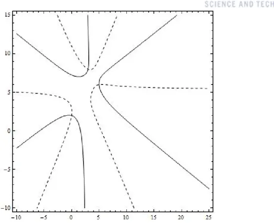
Figure 3-3: The basin of attraction of Newton Method shows the Newton fractal. This is an example of Julia sets associated to the Newton method forf(z) = (z−p1)(z−p2)· · ·(z−p5). The positions ofpi are denoted by white circles. Each different color region stands for a set of points

that converge to the same root by Newton method. Under the same (guiding) function it shows varied fractality depending on degree coefficientm.[74]

(34)

Figure 3-5: Newton paths generated from slightly different initial points near (3,3) (marked with a black circle): both eventually joins again at the target point (2,−1) (marked with a black square)[74].

(35)

Figure 3-6: The distribution of particles’ distance from a leading particle(after 50 times of iter-ations) follows the power law. All particles are initially located on the unit ball centered at the position of a leading particle. The straight lines are the least squares fitting line for log-log scale depending onm.

(36)

4

Newton Particle Optimizer

1

We propose Newton particle optimization(NPO) algorithm[74] and its convergence in this chap-ter. NPO is a population-based metaheuristic for global optimization problems. NPO enables the particles to search the space balancing between exploitation and exploration based on the chaotic nature of Newton method. Using chaos, NPO can control the irregular behavior with a few degree of freedom. This implies that NPO requires less random numbers than other stochastic metaheuristic methods. NPO is simple and powerful. In addition NPO is convergent fastly due to the convergence property of Newton method.

Complexity of the Newton paths can used to develop a global optimizer. It can be con-structed for a guiding functionf whose roots are the temporal best, or candidate for optimums, of population according to fitness functiong. By (3.3.1) all other particles are attracted to the temporal best ofg along the Newton paths. The sequences of particles’ positions are irregular, likely to wander around the temporal best, or sometimes take an unexpected jump away from them. If the temporal best is improved, the guiding functionf is updated accordingly. We up-date the position of particles with newly constructed guiding function whose roots are temporal best by Newton method at every iteration step.

4.1 Algorithm

We explain the algorithm of NPO in 2-dimensional search space first. A fitness function(or cost function) g :C→ Ris a function to be optimized. Each particle is a searching agent and the

population is N. Their positions are denoted as zi ∈C, 1≤i≤N. Each particle has a degree

coefficientmi∈C. By Newton method the position ofi-th particlezi is updated as following: zi ←zi−mi f(zi) f0₍_z i) (4.1.1) 1

This work will be published as: Jeong, S. and Kim, P, “A population based optimization method using Newton fractal.” Complexity,in press.

(37)

4.1 Algorithm

where f is a polynomial function that is defined to be a guiding function. Do not confuse f

withg, to be optimized. We can attract the particles near its roots by (4.1.1). That is why we need a root finding method like Newton method. The main concern is about how to construct the guiding functionf to apply (4.1.1) for all particles.

We easily come up with a guiding function in 2-dimensional space because of the complex system. A guiding functionf(z) is constructed as a polynomial of degreenwhose roots coincide withp1,· · · ,pn,as

f(z) = (z−p1)(z−p2)· · ·(z−pn). (4.1.2)

We can use the guiding function to search the space around its roots, possibly temporal best solutions, which are the candidate optimum.

At each iteration of the scheme, we choosenbest fitters with respect to the fitness function

g asleading particles. That is, we pick p1,· · · ,pn,such that

pi =zk whereg(zk) is the i-th minimum among g(z1)· · · , g(zN) (4.1.3)

fori= 1,· · · , n. It always needs notnbest fitters to be leading particles but the first best fitter should belong to the leading particles for monotonicity to the optimum.

Note that all the particles except the leading particles are attracted toward leading particles. Once the positions of all particles are updated, we examine their fitness to choose the next leading particlesp1,p2,· · · ,pn. Then we refresh the guiding functionf accordingly, and reapply

(4.1.1) to the particles. As long as the guiding function is a polynomial function, convergence of the algorithm is guaranteed from the convergence of the Newton’s method and the monotone convergence theorem. However, like other heuristic optimization methods, convergence here means convergence of the sequence of solutions in which all particles have converged to the points of leading particles, which is called ‘premature convergence’. In the search-space, those points may or may not be the optimum.

The pseudo code of the whole process is in Algorithm 1.

We want to extend the NPO to higher dimension, in Rd, d≥3. We set a guiding function f(x) = (f1(x),· · ·, fd(x))T wherex∈Rdandfi(x) is a real valued function inRd.Now (4.1.1)

becomes the multi-dimensional Newton method

x←x−M Df|−_x1 f(x), (4.1.4) whereM is ad-by-dconstant matrix andDf|−1

x is an inverse of the Jacobian matrix off atx.

The eigenvalues of M are related with local search tendency, m. As the eigenvalues increases from 0, the searching paths around the leading particles become more and more irregular as we

(38)

4.2 Searching manner of NPO

Algorithm 1 Newton Particle Optimization (inC)[74]

for each particledo

Initialize particle zi withmi.

end for

while maximum iterations or minimum error criteria is not attaineddo foreach particle do

Calculate fitness value g.

end for

Choose nbest membersp1,p2,· · · ,pn in the search domain.

Set the guiding function f(z) = (z−p1)(z−p2)· · ·(z−pn).

foreach particle do

zi ←zi−mi_ff0(₍z_zi) i)

end for end while

observed in 2-dimensional case in Figure 3-2 to 3-4. We will check the appropriate value of m

later in this chapter.

4.2 Searching manner of NPO

The searching manner of NPO is in contrast to conventional methods. We compare NPO with the two typical optimizers, gradient descent method(GDM) and PSO. When it comes to using population, NPO and PSO belong to same class and GDM belong to the other class. Before we move on to this topic, it needs to be mentioned that NPO and PSO are heuristic whereas GDM is algorithmic, which is the opposite concept of heuristic. Being algorithmic is following step-by-step procedure based on the information, not on the intuition or randomness. Other than that the algorithmic way requires more information than heuristic style, they have a dif-ferent type of uncertainty.

As a matter of fact, GDM has a hidden uncertainty which derives from the initial guess. GDM may give us different results depending on the initial condition not as long as the function to be optimized is convex. In order to keep the uncertainty from the initial guess off, it is safe to start with multi-agent as population-based methods do. Because the most expensive part of optimization is usually the evaluation of fitness, population-based methods are computationally heavy but it is worth using if the fitness function is complicated. Though population-based methods usually start with uniformly random distributed candidate solutions, the interaction among population lessens the impact of initial guess.

Population-based methods can relieve the uncertainty from initial guess, but most of population-based methods are stochastic and bring randomness to move particles. As we mentioned above, population-based methods are adaptable to solve the intricate problem. Without randomness, it is hard to take action for current situation flexibly. So most population-based methods include the generation of random numbers.

(39)

4.2 Searching manner of NPO

Figure 4-1: NPO Algorithm. (a)A dotted line is represented the hidden fitness function and the global optimum labeled by diamond shape should be found. (b)Distribute the particles in uniformly random manner. These particles are candidate solution and marked by white circle. (c)Evaluate the fitness of the particles. (d)Choose the top 3 best fitters as leading particles. Leading particles are marked with black square label. (e)Make the guiding function with leading particles. (f)Update the other particle’s positions near the best fitter by applying Newton method with guiding function.

(40)

4.3 Convergence of metaheuristics

With regard to randomness, NPO and PSO are different. NPO uses the property of chaos whereas PSO generates the random numbers to search the space. The biggest difference is the degree of freedom to control the stochasticity. NPO needs the random numbers for initialization of particles’ positions and their degree coefficient m. On the other hand, PSO needs random numbers at every iteration from the initialization step. This implies that NPO is less uncertain than PSO. In addition NPO can get the same result as long as the initial condition is same. As a population based method, NPO suppresses the uncertainty from every iteration but keeps the uncertainty from initial guess, like GDM.

From the structure of the algorithm, each particle in PSO compares the best current opti-mum with its own private best and makes a noisy crawling toward the target. The particles in NPO do not memorize their history and simply jump toward one of the best known optimums in a diverse way.

4.3 Convergence of metaheuristics

For convergence of metaheuristic methods, there are three types that should be considered. First is premature convergence, which means that the particles gather somewhere and stop moving before the stopping criteria is satisfied. We want to avoid this convergence because it results in getting trapped in local minima, leading to bad performance. Many metaheuristics have an issue of premature convergence. There are some researches proposed to avoid the premature convergence. Premature convergence of a global optimizer should be checked carefully.

Second is local convergence, which means that the particles converge to a local minimum. This is the basic ability to be expected to achieve for an optimizer. Third is global convergence, which means that the particles find a global minimum. This convergence is the most desired convergence but no algorithm can guarantee this convergence regardless of the characteristics of fitness functions. Generally it is hard to distinct whether the particles are prematurely vergent, locally convergent, or globally convergent. Without local convergence, the global con-vergence is also not guaranteed even for a convex function. Check the definition in the following.

Definition 4.3.1. (Particle’s convergence)[57] A particleiis said to be convergent if

lim

t→+∞xi,t =p

where xi,t is the position of particle i at time t, and p is the any fixed position in the search

space S. The optimizer is said to be ‘prematurely convergent’ if all particles are convergent. Let f :Rd →Rbe a measurable function to be optimized in the search spaceS⊂Rd. The

(41)

4.3 Convergence of metaheuristics function D is defined as D(yt, xi,t) = ( yt iff(g(xi,t))≥f(yt), g(xi,t) iff(g(xi,t))< f(yt) (4.3.1)

whereg(xi,t) denotes the application of an optimizer[57]. yt denotes the current global best at

timet. The following condition is a necessary condition for local and global convergence of an optimizer.

Definition 4.3.2. (Algorithm condition)[57]The mapping D :S×_Rd_→_S_{should satisfy}_f₍_D₍_{x, ξ}₎₎_≤

f(x) and if ξ ∈S, thenf(D(x, ξ))≤f(ξ).

From the construction, D is satisfying the algorithm condition.

Definition 4.3.3. (Optimality region)[57] The algorithm is said to have found a solution if it is

able to generate a point in the optimality region,R, defined as

R ={z∈S|f(z)< ψ+},

whereψ denotes the essential infimum off.

This following is the sufficient condition for convergence to a local minimum.

Definition 4.3.4. (Local convergence)[57] For anyxt∈Sthere exists a γ >0 and an 0< η≤1

such that

µt(dist(xt+1, R)≤dist(xt, R)−γ orxt∈R)≥η

Let{xt}∞t=0 be a sequence generated by the algorithm, D. Then

lim

t→∞P(xt∈R) = 1.

This following is the sufficient condition for convergence to a global minimum.

Definition 4.3.5. (Global convergence)[57] For any (Borel) subsetAof Swith m(A)>0,

∞ Y t=0 1−µt(A) = 0

(42)

4.4 Local convergence of NPO

by the algorithm, D, then

lim

t→∞P(xt∈R) = 1.

To understand how an optimizer finds the optimum effectively, it might be a good choice to study about the convergence of an optimizer. PSO keeps moving until all particles’ fitness values are same. Note that it does not mean the particles gather in a point. They can be scat-tered in some points as long as their fitness values are same. Whereas the particles of NPO can be scattered in a few points without reference to fitness values. NPO maintains the diversity of particles well.

Though PSO algorithm cannot guarantee the local convergence, it can be guaranteed with modification of the position of the global best particle only. F. van den Bergh et al. showed premature convergence of PSO and modified PSO to achieve local convergence[57]. This mod-ified PSO is referred to as guaranteed convergence PSO(GCPSO). For GCPSO, the update of global best particlexτ, whose index isτ, is

xτ,t+1=yt+wvτ,t+ρt(1−2rt),

where rt is randomly chosen from uniformly distributed [0,1]. The previous two terms in the

update equation is same with standard PSO algorithm. Outstanding modified part,ρt, is defined

as follows. ρt+1=      2ρt if #successes> sc 0.5ρt if #failures> fcand ρt> m ρt otherwise (4.3.2)

wherem represents the smallest allowable value ofρ, maybe the machine precision. A ‘failure’

occurs when f(ˆyt) ≥ f(ˆyt−1) and a ‘success’ occurs when f(ˆyt) < f(ˆyt−1). The number of

successes, or failures is reset to zero when the failure, or success happens, respectively.

4.4 Local convergence of NPO

Standard NPO is prematurely convergent. A guiding function has a neighborhood convergent to the roots, called radius of convergence, by Newton method. On the other hand, finding minimum within finite candidate solution is impossible for black box problems. Thus the particles stagnate before they find the minimum.

But it can be guaranteed with variation similar to the procedure of GCPSO in the previous section[57]. We call modified NPO as guaranteed convergence NPO(GCNPO). For NPO, there needs to keep updating the positions of leading particles to avoid premature convergence. This following theorem and its proof are similar to those of PSO[57].

(43)

4.4 Local convergence of NPO

Theorem 4.4.1. (Local convergence of GCNPO) GCNPO is locally convergent if the particle updated with

xτ,t+1 =yt+ρt(1−2rt)

belongs to leading particles as well as the global best particleyt does so. ρt is defined in (4.3.2)

andrt is a random number in[0,1]. By entry of random numbers, the particles keep moving in

any situation and search the space densely or sparsely.

Proof. Randomness, ρt part is exactly from the GCPSO[57]. This update is about sampling a

point from a hypercube whose length is 2ρcentered at temporal best,yt. Sinceρtis changing, we

denote ρinstead. Mk denotes that hypercube and µk denotes the uniform probability measure

defined on Mk. Premature convergence never happens because it keeps updating the position

of leading particles by randomness regardless of any interaction of particles or environment. We define a compact set

L0 ={x∈S:f(x)≤f(x0)} (4.4.1)

wherex0 is the particle who has the largest fitness value, defined as

x0 =argmaxxi{f(xi)}, i∈Z,1≤i≤N (4.4.2)

where N is the population. Then yt ∈ L0. And yt ∈ Mk. Thus m[Mk∩L0] >0. m denotes

the Lebesgue measure of a set. A non-degenerate sampling volumeµk with support Mk exists.

Now we check the local convergence of GCNPO.

S is compact and has a non-empty interior. Then so does L0. By definition, R ⊂ L0.

Because a closed subset of compact set is compact, R is compact with a non-empty interior.

Refer [57] in detail. We choose a ball, B0, centered at c0 in R. x0 is the argument of x ∈ L0

for the maximum distance with c0. B is the hypercube centered at c0 whose side length is 2(dist(c0, x0)−0.5ρ). C is the convex hull ofx0 and B0. The tangent line connecting B0 andx0

is the longest line of x0 and B0. This implies that the volume surrounded by any other convex hull made by any x∈L0 is greater than the volume ofC∩B. Therefore for any x∈L0,

µk[dist(D(ˆy, xτ), R)< dist(x, R)−0.5ρ]≥η=µ[C∩B]>0

A population-based optimization method using Newton fractal

A population-based optimization method

using Newton fractal

Soyeong Jeong

Department of Mathematical Sciences

Graduate School of UNIST

A population-based optimization method using

Newton fractal

A dissertation

submitted to the Graduate School of UNIST

in partial fulfillment of the

requirements for the degree of

Doctor of Philosophy

A population-based optimization method using

Newton fractal

Soyeong Jeong

This certifies that the dissertation of Soyeong Jeong is approved.

Abstract

Contents

List of Figures

List of Tables

1

Introduction

1.1

Overview

1.2

Global optimization problems

1.3

Summary of contents

2

Population-based Metaheuristics

2.1

Population-based metaheuristics

2.2

Applications of population-based methods

3

Exploration and Exploitation in

Chaos-based searches

3.1

Chaos v.s. randomness in optimization

3.2

Adoption of chaos in global optimizers

3.3

Chaos created by Newton method

4

Newton Particle Optimizer

1

4.1

Algorithm

4.2

Searching manner of NPO

4.3

Convergence of metaheuristics

4.4

Local convergence of NPO