Bayesian moment-based inference in a regression model with misclassification error By: Christopher R. Bollinger, Martijn van Hasselt
Bollinger, C. R. & Van Hasselt, M. (2017). Bayesian Moment-Based Inference in a Regression Model with Misclassification Error. Journal of Econometrics, 200(2), 282-294. DOI:
10.1016/j.jeconom.2017.06.011.
Made available courtesy of Elsevier: http://dx.doi.org/10.1016/j.jeconom.2017.06.011
This work is licensed under a Creative Commons Attribution-NonCommercial-NoDerivatives 4.0 International License.
Abstract:
We present a Bayesian analysis of a regression model with a binary covariate that may have classification (measurement) error. Prior research demonstrates that the regression coefficient is only partially identified. We take a Bayesian approach which adds assumptions in the form of priors on the unknown misclassification probabilities. The approach is intermediate between the frequentist bounds of previous literature and strong assumptions which achieve point
identification, and thus preferable in many settings. We present two simple algorithms to sample from the posterior distribution when the likelihood function is not fully parametric but only satisfies a set of moment restrictions. We focus on how varying amounts of information
contained in a prior distribution on the misclassification probabilities change the posterior of the parameters of interest. While the priors add information to the model, they do not necessarily tighten the identified set. However, the information is sufficient to tighten Bayesian inferences. We also consider the case where the mismeasured binary regressor is endogenous. We illustrate the use of our Bayesian approach in a simulated data set and an empirical application
investigating the association between narcotic pain reliever use and earnings.
Keywords: Binary misclassification | Partial identification | Bayesian bootstrap | Empirical likelihood
Article:
1. Introduction
In this paper we consider a regression model with a binary explanatory variable that is subject to measurement error: there is some nonzero probability that an observation is classified into the wrong category. Such a model is relevant, for example, for estimating treatment effects when compliance with treatment is not observed. Other examples include measuring the union wage differential Bollinger (1996), Bollinger and David (1997), Card (1996), Freeman (1984), measuring the impact of IT training and certification on earnings (Vakhitova, 2006), measuring the impact of disability status on earnings and employment (Kreider and Pepper, 2007), or
measuring the impact of food stamps (SNAP) on food security or health (Gundersen et al., 2012). Misclassification also occurs in survey data, which are known to suffer from response error
(Biemer et al. 1991; Bound et al., 2001). Failing to account for this problem may result in serious bias. If one is willing to impose a strong identifying assumption (for example, assuming that the misclassification rate is known or consistently estimable as in Aigner (1973)), it is possible to consistently estimate the parameters of interest. Some recent models have achieved identification when certain location parameters of the mismeasured variable are identified (Hu and Schennach, 2008). Hu (2008) provides an identification approach using instruments and (weak) restrictions on the misclassification rates, whereas Card (1996) uses validation data to obtain estimates of misclassification rates. In the absence of instruments, validation data or tight restrictions on misclassification rates, the parameter of interest is typically no longer point identified. In certain models, however, it may still be feasible to find identified and informative bounds for the parameter. A derivation of such bounds can be found in Klepper (1988a), Klepper (1988b) and Bollinger (1996).
Bounding results are obtained for models without additional assumptions on misclassification. However, imposing parametric distributional assumptions is typically undesirable; while these may lead to identification, the results are likely to be fragile. Differences in distributions may result in large changes in the estimates. Instead, as is the case for the model considered in this paper, informative bounds can be derived by only assuming that the second moments of the observed variables are finite. Unfortunately, the resulting bounds are often quite far apart. For example, our empirical application bounds the earnings gap associated with narcotic pain reliever use between $7618 and $3.1 million. Adding the assumption that drug use is not over-reported, the upper bound shrinks to $243,900. This example and earlier work by Bollinger (1996) demonstrate that additional information about the extent of measurement error has a substantial effect on the bounds of the identified region. While this is one form of useful information, in many cases the assumptions necessary for this approach may be difficult to justify. However, researchers may have information about the misclassification rates that can be formalized as a Bayesian prior distribution. In this paper, we examine the link between
information in the form of a prior and the implications for posterior distributions and inference. There is only a small literature on using Bayesian inference in set-identified models. One of the earliest contributions in this area is Erickson (1989). More recently, Poirier (1998) and Moon and Schorfheide (2012) consider a broad variety of models with non-identified parameters. In these models the data are informative about a set of reduced form parameters (we adopt the
terminology of Moon and Schorfheide (2012)). It is well known (e.g. Walker, 1969; Heyde and Johnstone, 1979) that in parametric models the posterior of these parameters is asymptotically normal. In the limit, the posterior distribution and the asymptotic distribution of the maximum likelihood estimator coincide. However, rarely are the reduced form parameters of primary interest. We will refer to the latter as “primary” parameters. In our context, these are the
regression parameters that determine the outcome model. In partially identified models, there is a mapping from primary parameters to reduced form parameters which is not one-to-one. From a Bayesian perspective, the posterior distribution of the primary parameters is only partially
updated. In fact, Poirier (1998) shows that the (marginal) posterior of the primary parameters is a weighted average of their conditional prior, given the reduced form parameters.
The analysis we propose here is different from previous work such as Moon and Schorfheide (2012) in that we consider likelihoods that are defined by a simple set of moment restrictions.
Thus, we do not impose distributional assumptions. As shown in van Hasselt and Bollinger (2012), even assumptions such as homoskedasticity can lead to a change in the identified set in the model studied here. Most non-Bayesian treatments of this model share the focus on moments. Rather than utilizing an approximate likelihood as in Liao and Jiang (2010), we incorporate two versions of a semiparametric likelihood that are particularly convenient in the context of moment functions. Depending on the prior information that the researcher entertains, inference can be based on the Bayesian bootstrap Rubin (1981), Chamberlain and Imbens (2003), or on the Bayesian exponentially tilted empirical likelihood (BETEL) approach of Schennach (2005). We focus on adding information to the model through the prior distributions on the misclassification rates. This is a natural approach to adding information and compliments the approach taken in Bollinger (1996), where (deterministic) information on the measurement error rates was found to tighten the identified region. In the context of our model, we assess how priors change the posterior distribution and hence change inference about the parameter of interest. We extend these results to allow for endogeneity. Here, in particular, we highlight that the prior provides identifying information that results in finite highest posterior density (HPD) intervals.
Partial or set identification requires a careful approach to inference. In practice, many authors (e.g. Bollinger, 1996) simply use standard confidence intervals for the estimated upper and lower bounds. There is a substantive difference, however, between inference about the identified set and inference about the parameter itself. For the case of a single parameter, Horowitz and Manski (2000) demonstrate how to construct a confidence region with a given (asymptotic) coverage probability for the entire identified set. Chernozhukov et al. (2007) extend these results to vector-valued parameters and a broader class of econometric models. Such confidence regions are conservative for the parameter itself. Imbens and Manski (2004) show how to construct the confidence set for a (scalar) parameter. Their method entails properly adjusting the critical value so that the coverage probability converges to the desired level uniformly over the parameter space. From a Bayesian perspective, it is natural to focus on inference about the regression parameters rather than the identified set. As such, we will compare our results to frequentist inference based on the work of Imbens and Manski (2004). As our results show, it is possible for Bayesian credible intervals to be strictly contained in frequentist confidence sets (Moon and Schorfheide, 2012).
The approach here is intermediate between the frequentist bounds, which incorporate no prior information on the parameters beyond the main model and the data, and cases where additional information such as bounds on misclassification rates or further distributional assumptions tighten the identified set. We examine priors that do not change the identified set yet lead to stronger inferential conclusions through a more concentrated posterior distribution and narrower highest posterior density intervals. We also demonstrate that approaches with strong information can be nested in the Bayesian prior, resulting in both a tightening of the identified set and a concentration of the posterior of the parameter of interest. The focus here is how information, stated in the form of a prior on the misclassification rates, sharpens the inference or identified set, as compared to the approach of Bollinger (1996).
Recently, several papers have addressed both misclassification errors and endogeneity of a binary explanatory variable Kreider et al. (2012), Frazis and Loewenstein (2003), Hu et al. (2015), Hu et al. (2016), Shiu (2016). In the model here, without further information about the
extent of the endogeneity, set identification fails and the model parameters are completely unidentified (Manski, 1995). We show how to incorporate endogeneity in the Bayesian model and calculate Bayesian credible intervals under different priors about the endogeneity. These priors can again be seen as incorporating different amounts of identifying information into the model. Here the identifying information results in finite HPD intervals which allow for
inference.
The remainder of this paper is organized as follows. Section 2 introduces the model, whereas Section 3 presents algorithms to sample from the posteriors, based on the Bayesian bootstrap and BETEL. We illustrate the use of these algorithms with simulated data in Section 4. In section 5 we expand the model to include endogeneity. In Section 6, we apply the algorithms to estimate the wage gap between individuals who use and those who do not use prescription pain relievers. Section 7 concludes.
2. The model
We consider a simple regression model with a single binary regressor taking values of zero or one. The regression coefficient in this case is the difference between two conditional means. It is possible to incorporate additional covariates into the analysis that follows, but such an extension complicates the notation and is not necessary to convey the main points. Our discussion here closely follows Bollinger (1996) and van Hasselt and Bollinger (2012), whose notation we adopt. The outcome for sampling unit i is given by
(1) where Xi∗∈{0,1} has a Bernoulli distribution with Pr{𝑋𝑖∗=1} = π and π ∈(0,1). The linearity of Eq. (1) is not restrictive because Xi∗ is binary. The regression coefficients satisfy α = E(Yi|Xi∗=0) and β = E(Yi|Xi∗ = 1) − E(Yi|Xi∗ = 0), and the model is saturated. We refer, throughout, to the parameters in this model as the regression parameters.
The binary covariate Xi∗ is not always observed. Instead, the data contain a variable Xi, where
(2) Here p is the conditional probability of observing a false positive while q is the conditional probability of observing a false negative. The difference Xi−Xi∗ is measurement error, which is non-classical because its conditional distribution depends on the value of Xi∗. Eq. (2) does represent the assumption, however, that the error is conditionally independent of the residual Ui. Because Pr{Xi = 1|Xi∗,Ui} = Pr{Xi = 1|Xi∗,Yi}, the misclassification error is conditionally (on Xi∗) independent of the outcome.1 Finally, the restriction p + q < 1 ensures that the covariance between Xi and Xi∗ is positive. Hence, the misclassification is not so extreme as to make Xi and Xi∗ independent (p + q = 1) or to reverse the categorical definitions (p + q >1).
Following Moon and Schorfheide (2012), we distinguish three sets of parameters in this model: (i) the regression parameters θ=(α, β, π, 𝜎𝑦2), (ii) the error probabilities p and q, and (iii)
the first two central moments (mean, variance, covariance) φ=(μX, μY, 𝜎𝑦2, σXY) of Xi and Yi.2 We assume that the goal is to make inference about θ, and inparticular β. The error probabilities are not of primary interest and can be considered nuisance parameters. The vector of moments (φ) is identified by the observed data and can be estimated by conventional methods. Following Moon and Schorfheide (2012), we refer to these as the reduced form parameters. Eqs. (1) and (2) imply the following functional relations between the three sets of parameters:
(3) From an identification perspective, the moments φ can be treated as known constants because they are nonparametrically identified and estimable through sample moments. The system (3) then has 4 equations in 6 remaining unknowns. Without further restrictions a unique solution for θ does not exist, and hence, θ is not identified. Different sets of additional restrictions can lead to identification. Chen et al. (2008) show that θ is identified if E(𝑈𝑖2|Xi∗) and E(𝑈𝑖3|Xi∗) are
independent of Xi∗. In this paper we base inference only on the model in Eqs. (1) and (2) and the restrictions that these equations imply. Consequently, our goal is to make inference about parameters that are not point identified.
Bollinger (1996) shows that despite the lack of point identification, the regression model and nuisance parameters are partially identified, in the sense that (i) these parameters can be bounded from above and below, and (ii) these bounds are nonparametrically identified (hence estimable). For example, assuming that β ≥ 0, it can be shown that
The interval between the lower and upper bounds is the identified set for β. Bollinger (1996) also presents bounds on p, q, α and π. Although all these bounds can be easily estimated, in practice they can be quite far apart, providing unsatisfying conclusions. A number of assumptions can be brought into the model which shrink the identified set. For example, in an application to
pollution exposure and health, Klepper (1988a) uses the restriction p = q, which tightens the upper bound. Bollinger (1996) discusses additional restrictions on (p, q) that further shrink the identified set and applies this to the union wage differential. van Hasselt and Bollinger (2012) show that homoskedasticity tightens the identified set and that homoskedasticity coupled with the assumption p = q identifies the model parameters. In each of these cases, the bounds are tightened because the upper bound represents extreme cases of highly asymmetric
misclassification (only one way or another) coupled with a variance of ui which is zero. In this paper, we focus on the wider bounds of Bollinger (1996), which are based on fewer assumptions. We do, however, consider priors that impose additional restrictions on (p, q) as well as priors that do not. It is relatively straight forward to modify our approach here, inconjunction with other assumptions such as error symmetry or homoskedasticity.
3.1. The likelihood, identification, and the posterior
We assume that an i.i.d. sample Dn = {𝑋𝑖, 𝑌𝑖}𝑖=1𝑛 is observed from the model in (1) and (2). There are different ways to parameterize the likelihood in terms of θ, φ, and (p, q). In this section we use the likelihood f(Dn|θ, p, q), parameterized by the regression parameters and the error probabilities. However, the following arguments apply to other parameterizations as well. Given a prior distribution f(θ, p, q), the posterior distribution can be written as f(θ, p, q |Dn) ∝ f(Dn|θ, p, q)f(θ, p, q). One way to proceed is to assume that the regression error Ui Eq. (1) has a known distribution, for example Ui|𝑋𝑖∗ ∼ N(0, 𝜎𝑈2). Although such aparametric assumption is often made for convenience, it has a strong impact on the identification (or lack thereof) of the model
parameters. In the context of a partially identified, semiparametric model, parametric restrictions can either significantly reduce the size of the identified set or lead to point identification. Related to this, statistical inference, whether Bayesian or not, can be quite sensitive to parametric
assumptions.
In the approach we take here, we do not assume that the likelihood is a known parametric distribution. Instead, we examine to what extent the econometrician can learn about θ while maintaining a weak set of assumptions about the statistical model generating Dn. We focus on the reduced form parameters φ, which are nonparametrically identified and can be consistently estimated from the data. Knowledge of φ, however, is not sufficient to identify θ or (p, q). This situation can be characterized by likelihoods that satisfy
Where φ, θ, and (p, q) are subject to the system of equations in (3). The key insights are that (i) the mapping from φ to θ is not one-to-one, and (ii) the likelihood function is determined by φ alone. Instead of conditioning on the full vector (φ, θ, p, q) on the left-hand side of (4), we can condition on φ and any two elements of (θ, p, q), because the system in (3) then determines the remaining parameters. Thus, instead of (4), we can also write f(Dn|φ, p, q) = f(Dn|φ), or f(Dn|φ, α, β) = f(Dn|φ), etcetera
Suppose the econometrician has prior beliefs about the misclassification probabilities p and q and the moments φ, expressed by a distribution f(φ, p, q). From Bayes’ rule and Eq.(4), it follows that
(5) This shows that the posterior distribution factors into the product of the marginal posterior of the identified parameters φ and the conditional prior of the non-identified parameters p and q.3 This is a crucial feature of posterior distributions in models with non-identified parameters and has been discussed by many authors (e.g., Kadane, 1974; Poirier, 1998; Moon and Schorfheide, 2012). The sample is informative about φ, because in large samples f(φ|Dn) becomes less dispersed and concentrates around some value. On the other hand, updating beliefs about (p, q) occurs only through updating the value of φ in the conditional prior f(p, q|φ). Moreover, if Sφ is the support of f(φ|Dn), then it follows from (5) that
(6) Hence the marginal posterior of (p, q) is a weighted average of the conditional prior where the weight function is the posterior of φ. In large samples, the posterior of φ will concentrate around some value, say φ∗. Eq. (6) shows that then the posterior of (p, q) will concentrate around f(p, q|φ∗).
3.2. The Bayesian bootstraps
We consider two versions of a semi-parametric likelihood that only satisfies the simple moment restrictions E[g(Xi,Yi,φ)] = 0,where
A first option is to use the Bayesian bootstrap, introduced by Rubin (1981) and adapted by Chamberlain and Imbens (2003). The main idea is as follows: suppose (Xi,Yi) has a discrete joint distribution with a finite support. Let {zj;j = 1,..., J} be the collection of support points. Since most data are measured with finite precision (i.e., discretely) and because J can be large, the assumption of a finite number of support points is not very restrictive (Chamberlain and Imbens, 2003, p. 12). Let ξ= (ξ1,...,ξJ) be a set of multinomial probabilities with ξj = Pr{(Xi,Yi) = zj}. The moment restrictions can then be written as
(7) Through this set of equations, a prior (posterior) distribution for ξ induces a prior (posterior) for φ. Defining nj = ∑𝑖=1𝑛 I{(Xi,Yi)=zj}as the number of observations in the sample equal to zj, the multinomial likelihood for the sample is f(Dn|ξ) = ∏𝑗=1𝐽 𝜉𝑗𝑛𝑗.4 The natural conjugate prior for ξ is the Dirichlet distribution D(c) with parameters c = (c1,...,cJ):
Chamberlian and Imbens (2003) show that the improper prior that is obtained when cj → 0 for all j has some desirable properties. With this choice of c, and using the multinomial likelihood, it follows that the Dirichlet posterior of ξ is given by
This posterior, together with the set of restrictions in (7), imply that the posterior of φ is a multivariate B-spline (Dahmen and Micchelli, 1981). It is easy to generate random draws from this posterior, as we will discuss shortly. However, we first turn to the posterior of the remaining parameters. We focus on p and q, assuming (as we did in the previous section) that the
econometrician has prior beliefs about the misclassification probabilities. Given a random draw from the posterior of (p, q, φ), a value of θ = (α,β,π,𝜎𝑈2) can be calculated from the system in (3). This value then constitutes a draw from the posterior of θ. The likelihood as a function of (φ, p, q) can be calculated by integrating out multinomial probabilities ξ over their conditional prior with support Ξ:
(8) From Bayes’rule,
Consider the conditional prior f(p,q|φ,ξ) and suppose we change the distribution of (Xi,Yi) by changing ξ. This affects the moments of (Xi,Yi) and informs us about p and q (and θ), because it changes the bounds of the identified set. However, it adds no information about the location of p and q within these bounds. In other words, the information that ξ carries about the
misclassification rates operates only through the reduced form parameters φ, so that f(p, q|φ,ξ) = f(p,q|φ). Substituting this into the previous display and (8), we then find
Thus, the Bayesian bootstrap likelihood function satisfies (4), and the posterior of (φ,p,q) satisfies (5). Random draws from the posterior f(φ,p,q|Dn) can now easily be generated, as described in the following algorithm.
Algorithm 1. If f(p,q|φ) is the conditional prior distribution of p and q given φ, then a random draw from the Bayesian bootstrap posterior distribution of (φ,p,q) can be obtained as follows:
1. Randomly generate a set of independent variables {𝑢𝑖}𝑖=1𝑛 from the unit exponential distribution.
2. Calculate
Then ξj has a Gamma distribution with parameters nj and 1, and (ξ1,...,ξJ) ∼ D(n1,...,nJ). 3. Calculate the solution φ∗ to the system of equations
4. Generate a random draw (p∗,q∗) from the conditional distribution f(p,q|φ∗). The value (φ∗,p∗,q∗) is a draw from the posterior.
Note that substituting (φ∗,p∗,q∗) into the system (3) and calculating the solution (α∗,β∗π∗, 𝜎𝑈2∗) yields a random draw from the (degenerate) posterior of all model parameters. Finally, we note again that step 4 in the algorithm is formulated in terms of the conditional prior of p and q given φ. If the econometrician wants to use prior beliefs about, for example, α and β, a
conditional prior distribution f(α,β|φ) would be used in step 4. Posterior draws (φ∗,α∗,β∗) and the mapping (3) then immediately yield the posterior draws (p∗,q∗,π∗,𝜎
𝑈2∗).
A second semiparametric likelihood that only satisfies a set of moment restrictions is the Bayesian exponentially tilted empirical likelihood (BETEL) of Schennach (2005). It is based on the idea of maximum entropy estimation (e.g. Kitamura and Stutzer, 1997; Imbens et al., 1998). In particular, the entropy of a multinomial likelihood supported on the sample is maximized, subject to the moment restrictions. Let gi(φ) be shorthand for g(Xi,Yi,φ). Fora given value of φ, the multinomial probabilities ξ∗(φ) solve the following problem:
provided zero lies in the convex hull of {𝑔𝑖(𝜑)}𝑖=1𝑛 . For a given value of φ, the solution is given by
where λ is a vector of Lagrange multipliers. In practice, the multi-nomial probabilities are easy to calculate, because λ(φ) minimizes a strictly convex function. The multinomial likelihood
∏𝑖−1𝑛 𝜉𝑖∗(φ) can be used to calculate the posterior of φ:
(9) The likelihood function has solved a maximum entropy problem that only depends on the value of φ. As such, the BETEL likelihood function also satisfies (4) and (5).
As with the Bayesian bootstrap, the decomposition in Eq. (5) suggests a simple way to generate a sample from the BETEL posterior. First, generate a random draw φ∗ from the posterior in (9); second, generate a random draw (p∗,q∗) from the conditional prior f(p,q|φ∗). While the second step is straight forward, the first step is slightly more involved compared to the Bayesian bootstrap. We use the Metropolis–Hastings algorithm (Gilks et al., 1996) to generate an
approximate sample from f(φ|Dn), similar to the approach of Lancaster and Jun (2010). In the second step, a draw is generated from a conditional prior. This leads to the following algorithm.5 Algorithm 2. Let f(φ) be the prior of φ and let f(p,q|φ) be the conditional prior. Given the
parameter values (φt,pt,qt) at iterationt, generate (φt+1,pt+1,qt+1) as follows:
1. Generate a random draw from a distribution g(φ|φt) that depends on the current value φt.
2. Calculate the multinomial BETEL likelihood at the values φt and ,and the ratio
3. Set
4. Generate a random draw (pt+1,qt+1) from the distribution f(p,q|φt+1). 5. Set t = t+1, return to step 1 and repeat.
Algorithm 2 generates a Markov chain of values for (φ,p,q).These values can be used to calculate a set of values for θ, which represents an approximate sample from the posterior f(θ|Dn). The distribution g is the “proposal distribution” that generates candidates for new states in the Markov chain for φ. At each iteration, the chain either moves to the new state with probability min{1,rt} or remains in its current state φt with probability 1−min{1,rt}. In practice, the proposal distribution is often chosen such that around 25% − 30% of the generated draws from g are accepted as new states in the Markov chain (Gelmanetal.,1995). Intuitively, if rt ≈ 0 the Markov chain remains mostly stuck in certain states, whereas if rt ≈ 1 the chain mostly consists of values drawn from g. In both cases the simulated values will likely be a poor approximation to the posterior distribution.
The posterior of φ will be close to normal in large samples. A natural and convenient choice for g(φ|φt) is therefore the N(φt,c2𝑉n/n) distribution, where c2 is a dispersion constant (Gel-manetal., 1995, p.334), and Vn is an estimator of the asymptotic variance of the method-of-moments estimator of φ (Lancaster and Jun, 2010). In this case, g( |φt) = g(φt| ) and the ratio rt in Algorithm 2 simplifies to the ratio of posteriors f( |Dn)/f(φt|Dn).
The major difference between BETEL and the Bayesian boot-strap is that BETEL allows a researcher to start with prior beliefs about (θ, p, q). The mapping in (3) and a change of
variables can be used to calculate the prior f(φ, p, q). An application of Algorithm 2 then yields an approximate sample from the posterior of (φ, p, q) and, through the system (3), from the posterior of the regression parameters θ. On the other hand, the Bayesian bootstrap cannot be used with arbitrary prior beliefs about (θ, p, q). In particular, there is no way to explicitly incorporate prior beliefs about φ.6 The Bayesian bootstrap is applicable if the econometrician specifies the conditional prior of any two parameters in (θ, p, q), given φ. For example,
Algorithm 1 shows how a given conditional prior f(p, q|φ) can be used to generate a sample from the posterior f(φ, p, q|Dn).
In some cases BETEL maybe the preferred approach because of its flexibility in terms of specifying the prior distribution. In other cases, the econometrician may view the Bayesian bootstrap as the easier approach because it requires fewer prior inputs (i.e., the conditional prior f(p, q|φ) instead of the full joint prior f(p, q, φ)). However, if the same conditional prior f(p, q|φ) isused for BETEL and for the Bayesian bootstrap, we expect the posteriors to be similar in large samples. BETEL requires a prior f(φ),but in large samples its impact is negligible and the posterior of φ concentrates around some value φ∗. In the Bayesian bootstrap, the prior f(φ) is not well defined, but the posterior of φ also concentrates around φ∗. From Eq. (6), in both approaches f(p, q|Dn) converges to f(p, q|φ∗).
3.4. A selection of priors
In this section we present several priors f(p, q|φ) that could be used in practice, reflecting different beliefs about misclassification rates. In Sections 4 and 6 these priors will be used in a simulation example and an empirical application. Conditional on φ, the probabilities p and q are bounded, and these bounds must be reflected in the support of the (conditional) prior distribution. Specifically, the restriction 𝜎𝑈2 ≥ 0 and the mapping in (3) imply the inequality
(10) where 𝜌𝑋𝑌2 is the squared correlation between Xi and Yi. Since (p, q) has to satisfy (10), the error rates cannot be independent in the prior. Bollinger (1996) shows that the maximum possible value of p occurs at q=0. In that case, 0≤p≤p∗(φ), where p∗(φ) = μX(1−𝜌
𝑋𝑌2 ). From (10), it can also be shown that for a given value of p, the bounds on q are 0≤q≤q∗(p, φ),where
An approach which has intuitive appeal is to base the priors of p and q on the uniform
distribution. The imposition of any prior distribution imposes information about the parameters. The bounds in Bollinger (1996) represent the fully agnostic case of no prior information (one can think of this as the case representing the union of all possible priors). The uniform prior imposes information in the form that all values have the same likelihood. An implication of this is that the probability of no measurement error is zero. Note that we construct the priors conditional on the reduced form parameters φ. We construct the joint prior as the product of a uniform prior for p given φ, and a uniform prior for q given p and φ.7 This results in the following prior, which we label “uniform”.
(11) In many cases, researchers have information that leads them to believe that misclassification rates are more likely to be concentrated among lower values of p and q. While inference could be based on imposing known upper bounds on the misclassification rates (as in Bollinger, 1996), this clearly rules out the (remote) possibility that these rates exceed the chosen thresholds. A probabilistic approach to incorporating this information is to use a “power” type distribution for
the prior. As with the uniform, the probability of p=q=0 (no measurement error) is zero.
However, the probability of measurement error for sets of (p, q) near the upper bound is very low as well. Our second “power” prior is then:
(12) In cases where researchers believe the misclassification rates are likely to be below a certain value but otherwise do not want to make the claim that the very lowest values are most likely, they may opt for a mixture of uniforms. Indeed, this prior allows researchers to place a high likelihood that the misclassification rates are below some threshold but does not rule out higher rates, unlike the approach of Bollinger (1996). In our third prior, we therefore suppose that p ≤ ̄p with probability λ1 (provided ̄p < p∗(φ)) and, conditional on p, that q ≤ ̄q with probability λ2 (again, provided ̄q < q∗(p,φ)). Thus, p and q may exceed these bounds (though they are still subject to p∗(φ) and q∗(p,φ)), but this only happens with probabilities of (1−λ1) and (1−λ2) respectively. This leads to the following prior with a uniform mixture structure.
(13) Thus, if the upper bounds p∗(φ) and q∗(p,φ) exceed ̄p and ̄q respectively, the priors are mixtures of uniform distributions. Otherwise, the priors reduce to f1(p|φ) and f1(q|p,φ)
An even stronger case combines the certainty bounds of Bollinger (1996) and the uniform distribution of prior 1. If the econometrician believes that p ≤ ̄ p and q ≤ ̄q with certainty then this belief can be expressed by the “bounded uniform” prior
(14) Finally, in some cases it may be reasonable to assume that misclassification is one-sided, in the sense that false negatives do not occur and q=0. For example, in the empirical application considered in Section 6, the binary variable is an indicator for abstinence from prescription pain
reliever (a value of 1 indicates no use, or abstinence of prescription pain reliever). There is reason to believe that few claim drug use in this survey when indeed they are not using. One can also extend the general idea to a prior where p=0. This may apply in food stamp programs, where there is little incentive to report participation when one does not participate (Bollinger and
David, 1997). If, at the same time, p is believed to be less than ̄p, we can use the prior
(15) For the purpose of sampling from the posterior, Algorithms 1 and 2 simplify slightly because no random draws of need to be generated.
We note that when moving from f1 to f2 to f3, we increase the amount of information contained in the prior without changing the identified set. While Bollinger (1996) considered how bounds on the misclassification rates change the identified set, this represents an
intermediate case, where the information is not strong enough to change the identified set but is strong enough to affect the Bayesian analysis through the posterior. In the cases of f4 and f5, we impose known upper bounds on the misclassification rates which also change the identified set. It is important to distinguish between cases where the prior does not change the identified set, and cases like f4 and f5 where the prior changes the identified set.
4. A simulation example
In this section we provide an example with simulated data. The example aims to illustrate the relationship between the prior and the posterior rather than to present a full Monte Carlo study. In our Bayesian analysis, we calculate the 95% highest posterior density (HPD) interval. This interval contains 95% of the posterior probability and the highest values of the posterior density. Thus, it is the tightest 95% band one can form with the posterior. Reporting the 95% HPD interval is common practice in the empirical Bayesian literature. For comparison purposes, we also calculate frequentist 95% confidence intervals for the parameters (Imbens and Manski, 2004).
In the simulation, we use the following values for the model parameters: α=β=1, 𝜎𝑈2 = 0.63, and π = 0.3. This implies an R-squared in the regression equation of 0.25. The
misclassification probabilities are p = 0.15 and q = 0.09. These are relatively high compared to many empirical settings (for one review, see Bound et al., 2001). We generate a sample of 1000 observations, where the outcome Yi is calculated according to Eq.(1) and the misclassified variable Xi is generated, conditional on 𝑋𝑖∗, according to Eq.(2). The calculation of the HPD intervals is based on 10,000 simulated draws from the Bayesian bootstrap and BETEL posteriors.
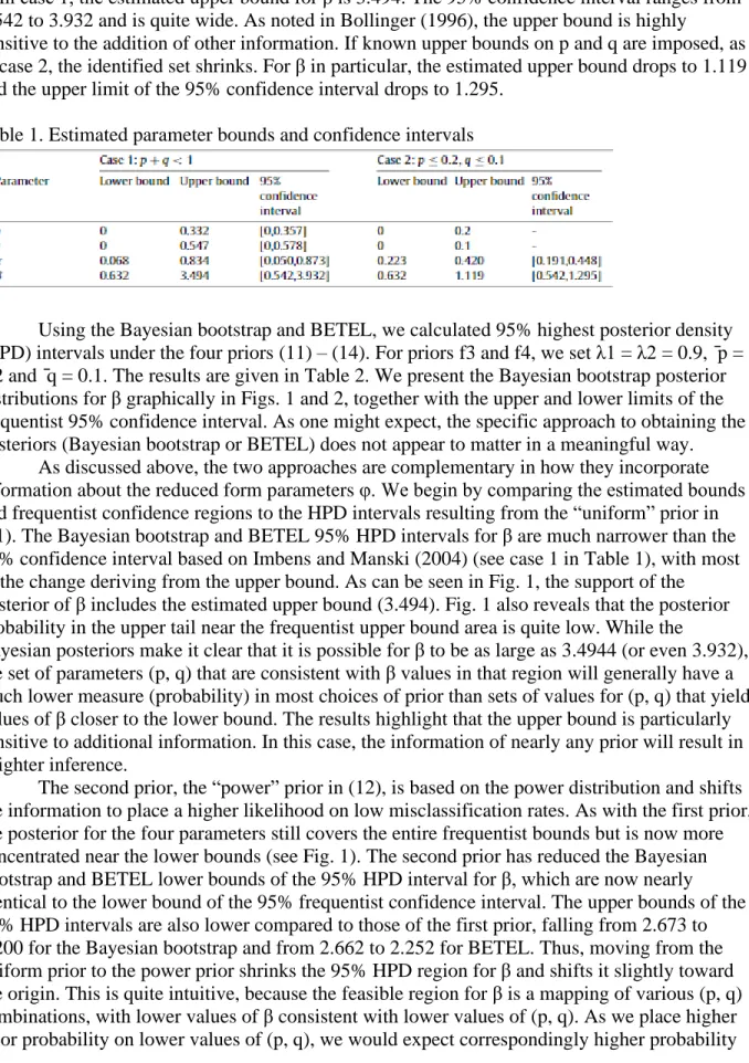
The estimated bounds and 95% confidence intervals for (p, q, π, β) are given in Table 1. The estimates were calculated using the results derived in Bollinger (1996), whereas the intervals were calculated using the method suggested by Imbens and Manski (2004). One should use caution in comparing these intervals. The Imbens–Manski confidence intervals are only affected by (sampling) uncertainty in the identified parameters (φ), whereas the HPD intervals are
affected by uncertainty about φ and the conditional prior of (p, q). The uncertainty about φ in both cases is relatively small, given the sample size and low variances. In the columns labeled ‘case1,’ the estimated bounds and confidence intervals were calculated under the assumption that p+q < 1 (see Eq. (2)). In the columns labeled ‘case2’, these were calculated using the additional information that p ≤ 0.2 and q ≤ 0.1. Throughout this discussion, we will focus on the parameter
β. In case 1, the estimated upper bound for β is 3.494. The 95% confidence interval ranges from 0.542 to 3.932 and is quite wide. As noted in Bollinger (1996), the upper bound is highly
sensitive to the addition of other information. If known upper bounds on p and q are imposed, as in case 2, the identified set shrinks. For β in particular, the estimated upper bound drops to 1.119 and the upper limit of the 95% confidence interval drops to 1.295.
Table 1. Estimated parameter bounds and confidence intervals
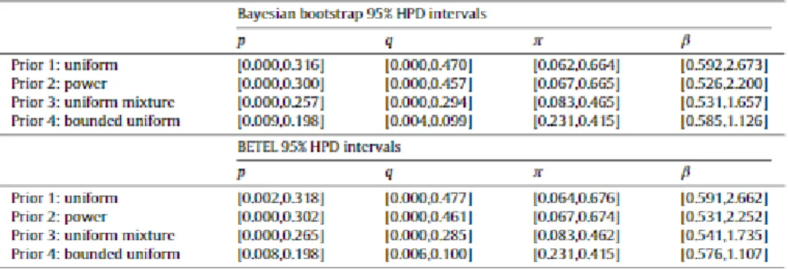
Using the Bayesian bootstrap and BETEL, we calculated 95% highest posterior density (HPD) intervals under the four priors (11) – (14). For priors f3 and f4, we set λ1 = λ2 = 0.9, ̄p = 0.2 and ̄q = 0.1. The results are given in Table 2. We present the Bayesian bootstrap posterior distributions for β graphically in Figs. 1 and 2, together with the upper and lower limits of the frequentist 95% confidence interval. As one might expect, the specific approach to obtaining the posteriors (Bayesian bootstrap or BETEL) does not appear to matter in a meaningful way.
As discussed above, the two approaches are complementary in how they incorporate information about the reduced form parameters φ. We begin by comparing the estimated bounds and frequentist confidence regions to the HPD intervals resulting from the “uniform” prior in (11). The Bayesian bootstrap and BETEL 95% HPD intervals for β are much narrower than the 95% confidence interval based on Imbens and Manski (2004) (see case 1 in Table 1), with most of the change deriving from the upper bound. As can be seen in Fig. 1, the support of the posterior of β includes the estimated upper bound (3.494). Fig. 1 also reveals that the posterior probability in the upper tail near the frequentist upper bound area is quite low. While the
Bayesian posteriors make it clear that it is possible for β to be as large as 3.4944 (or even 3.932), the set of parameters (p, q) that are consistent with β values in that region will generally have a much lower measure (probability) in most choices of prior than sets of values for (p, q) that yield values of β closer to the lower bound. The results highlight that the upper bound is particularly sensitive to additional information. In this case, the information of nearly any prior will result in a tighter inference.
The second prior, the “power” prior in (12), is based on the power distribution and shifts the information to place a higher likelihood on low misclassification rates. As with the first prior, the posterior for the four parameters still covers the entire frequentist bounds but is now more concentrated near the lower bounds (see Fig. 1). The second prior has reduced the Bayesian bootstrap and BETEL lower bounds of the 95% HPD interval for β, which are now nearly identical to the lower bound of the 95% frequentist confidence interval. The upper bounds of the 95% HPD intervals are also lower compared to those of the first prior, falling from 2.673 to 2.200 for the Bayesian bootstrap and from 2.662 to 2.252 for BETEL. Thus, moving from the uniform prior to the power prior shrinks the 95% HPD region for β and shifts it slightly toward the origin. This is quite intuitive, because the feasible region for β is a mapping of various (p, q) combinations, with lower values of β consistent with lower values of (p, q). As we place higher prior probability on lower values of (p, q), we would expect correspondingly higher probability
on lower values of β. We also note that the 95% HPD interval is not necessarily contained within the frequentist 95% confidence interval. While the addition of prior information often shrinks the HPD interval by lowering the upper bound, the effect on the lower bounds is modest. However, we do find that the length of the HPD interval is always substantially less than the length of the frequentist confidence interval.
The third prior, the uniform mixture distribution in (13), places even higher probabilities on lower values of (p, q). Compared to the power distribution, it reduces the overall probability of p > 0.2 and in particular concentrates probability on q < 0.1. As can be seen in both Fig. 1 and Table 2, this further concentrates the posterior and shrinks the 95% HPD intervals for β, with most of the change coming from the much tighter upper bound (1.657 for the Bayesian bootstrap and 1.735 for BETEL).
The fourth prior, the bounded uniform distribution in (14), results in a change in the identified set, tightening the asymptotic and estimated bounds (compare case 1 and case 2 in Table 1), and shrinking the frequentist confidence interval. However, the frequentist confidence interval of (0.542, 1.295) is still wider than the 95% HPD intervals (0.585, 1.126) from the Bayesian bootstrap and (0.576, 1.107) from BETEL. While the magnitudes of the differences are small, the best view of these is as a percentage change, as in practice these regions have larger scales. Thus, the HPD intervals from the Bayesian bootstrap and BETEL are about 28% smaller than the frequentist confidence interval. In Fig. 2, observe that the resulting posterior is more centered in the identified set than the first three priors. Clearly, the major gain of bounding the misclassification probability lies in tightening the identified set. The Bayesian HPD bounds associated with priors 1,2, and 3 are based on a weaker assumption: high values of (p, q) are allowed but discounted as less likely.
In summary, the results here reinforce those of Bollinger (1996) in that they demonstrate how the addition of information changes the inferences that can be made about the unidentified parameters. Even small changes in information can have large impacts on potential conclusions. Adding information which does not change the identified set has important impacts on the conclusions one might draw using posteriors. Priors that concentrate probability provide stronger conclusions. We suggest that the use of a prior and a Bayesian approach is a reasonable way to include information about the measurement error process, in cases where the information is not strong enough for identification yet cannot easily be incorporated into the frequentist bounds. Table 2. 95% HPDs from t he Bayesian bootstrap and BETEL
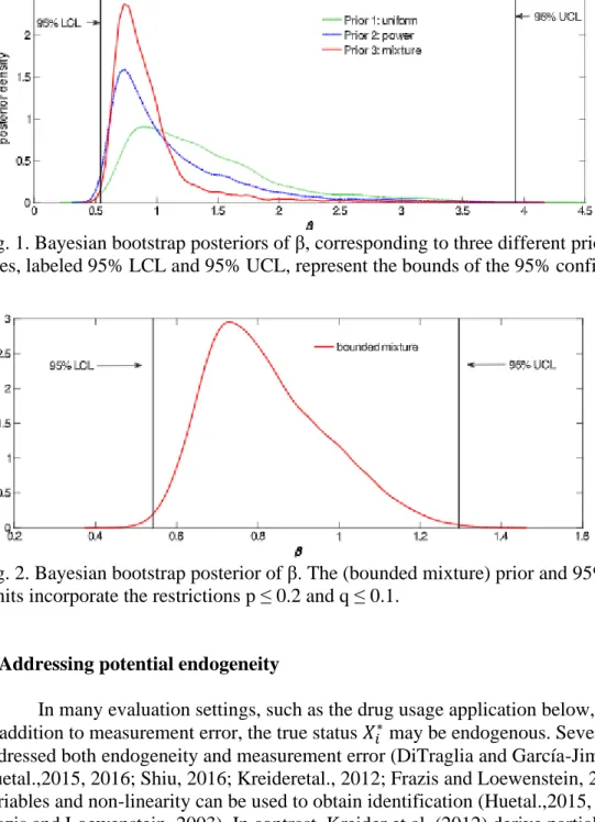
Fig. 1. Bayesian bootstrap posteriors of β, corresponding to three different priors. The vertical lines, labeled 95% LCL and 95% UCL, represent the bounds of the 95% confidence interval.
Fig. 2. Bayesian bootstrap posterior of β. The (bounded mixture) prior and 95% confidence limits incorporate the restrictions p ≤ 0.2 and q ≤ 0.1.
5. Addressing potential endogeneity
In many evaluation settings, such as the drug usage application below, concern arises that in addition to measurement error, the true status 𝑋𝑖∗ may be endogenous. Several papers have addressed both endogeneity and measurement error (DiTraglia and García-Jimeno, 2015 a, b; Huetal.,2015, 2016; Shiu, 2016; Kreideretal., 2012; Frazis and Loewenstein, 2003). Instrumental variables and non-linearity can be used to obtain identification (Huetal.,2015, 2016; Shiu,2016; Frazis and Loewenstein, 2003). In contrast, Kreider et al. (2012) derive partial identification results when the dependent variable is binary. In this case, the slope coefficient (β) in the model is not identified without further assumptions. In most applications, additional assumptions are brought to bear to obtain identification or at least to obtain set identification. In this section we use additional assumptions in the form of a Bayesian prior to allow for inference. In contrast to results in our previous sections, the posterior of β covers the real line. However, stronger priors lead to more concentrated posteriors and the HPD interval shrinks as additional information is incorporated. While this certainly does not “solve” the identification problem, it formalizes informational content from two issues, which provides an approach useful to researchers.
This adds a single new parameter (γ) and maintains the assumption that E(Ui) = 0. The parameterization of E(Ui|𝑋𝑖∗) is general, given the binary nature of 𝑋𝑖∗. This approach differs from Erickson (1989) who derives posteriors when there is correlation between the measurement error of a continuous regress or and the residual error Ui. We can rewrite the model
where now E(𝑈𝑖∗|𝑋𝑖∗) = 0 and E(𝑈𝑖∗2) < ∞. This returns us to the original model from Section 2, and all previous bounding results now apply to β∗ = β + γ. In many applications, there would be little to no prior information about the value of γ. In that case, β cannot be bounded and is
completely unidentified. However, if the researcher is able to formulate prior bounds on γ, then β becomes partially identified (DiTraglia and García-Jimeno, 2015a).
The posteriors in Section 3 and the simulations in Section 4provide a posterior for β∗. Thus, for any given value of γ, a distribution for β=β∗ − γ can be obtained. By adding a prior for γ, the posterior of β follows directly from the joint posterior of (β∗,γ). As before, let φ be the vector of identified, reduced form parameters. An argument similar to that of Section 3.1 can be used to show that
A draw from the posterior of β can therefore be obtained as follows. First, generate a draw from the Bayesian bootstrap of BETEL posterior of (φ, β∗), as in Sections 3.2 and 3.3. Second, draw a value γ from its conditional prior f(γ|β∗, φ) and calculate β = β∗ − γ. Because γ is completely unidentified, it may be reasonable to assume that γ is independent of β∗ and φ in the prior. We use this in the examples below and draw γ directly from its marginal prior. This prior can include bounds as well, which serve to set identify β. Alternatively, the researcher may prefer a prior that incorporates dependence between γ and β∗. This would be reasonable if there is prior knowledge about the likely magnitude of the endogenous effect (γ) relative to the causal effect (β). In this case, the researcher would have to separate, in a probabilistic sense, the association between 𝑋𝑖∗ and Yi into part endogenous effect and part causal effect. Regardless of the prior specification for γ, it will have a notable influence on the posterior of β.
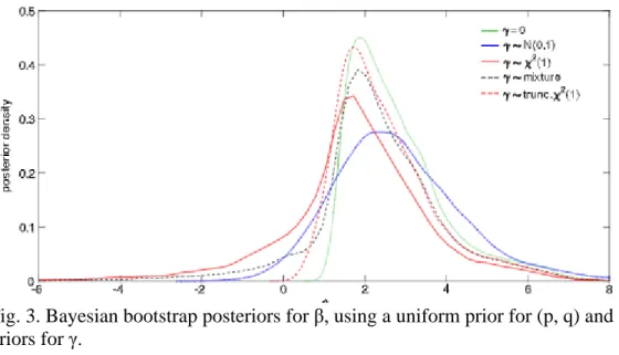
We extend the simulations in Section 4 to explore a variety of priors on γ, using a simulated data set with γ = 1. The remaining aspects of the data generating process are the same as those in Section 4. We focus on the uniform prior for the measurement error portion, and highlight the implications of five different priors on γ: (i) a point mass at γ = 0, which assumes that 𝑋𝑖∗ is exogenous; (ii) γ ∼ N(0, 1); (iii) γ ∼ χ2(1), a chi-square distribution with 1 degree of freedom; (iv) a 50-50 mixture of a point mass at zero and a χ2(1) distribution, (v) a χ2(1) distribution right-truncated at 1 (which is the 67 percentile of the χ2(1) distribution). Each of these priors represents different assumptions about the potential for endogeneity. In the case of the normal, it allows for both positive and negative endogeneity, but concentrated on low values of γ. The chi-square prior assumes that there is positive endogeneity, while the mixture allows
for a 50% probability that there is no endogeneity and a 50% probability that endogeneity is positive. Finally, the truncated chi-square prior assumes positive endogeneity with a known upper bound.
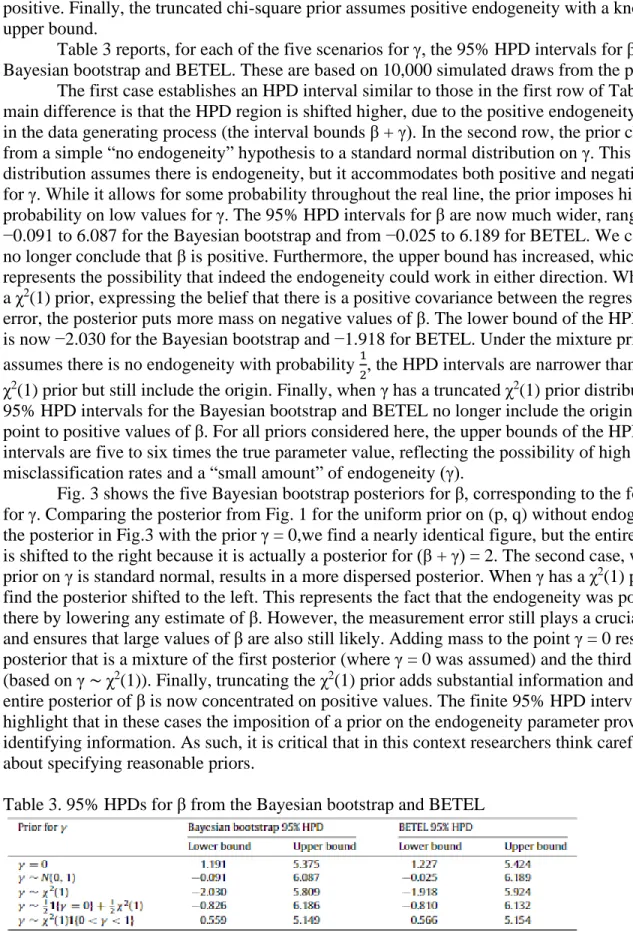
Table 3 reports, for each of the five scenarios for γ, the 95% HPD intervals for β from the Bayesian bootstrap and BETEL. These are based on 10,000 simulated draws from the posterior.
The first case establishes an HPD interval similar to those in the first row of Table 2. The main difference is that the HPD region is shifted higher, due to the positive endogeneity present in the data generating process (the interval bounds β + γ). In the second row, the prior changes from a simple “no endogeneity” hypothesis to a standard normal distribution on γ. This
distribution assumes there is endogeneity, but it accommodates both positive and negative values for γ. While it allows for some probability throughout the real line, the prior imposes higher probability on low values for γ. The 95% HPD intervals for β are now much wider, ranging from −0.091 to 6.087 for the Bayesian bootstrap and from −0.025 to 6.189 for BETEL. We can now no longer conclude that β is positive. Furthermore, the upper bound has increased, which
represents the possibility that indeed the endogeneity could work in either direction. When γ has a χ2(1) prior, expressing the belief that there is a positive covariance between the regressor and error, the posterior puts more mass on negative values of β. The lower bound of the HPD interval is now −2.030 for the Bayesian bootstrap and −1.918 for BETEL. Under the mixture prior that assumes there is no endogeneity with probability 1
2, the HPD intervals are narrower than for the χ2(1) prior but still include the origin. Finally, when γ has a truncated χ2(1) prior distribution, the 95% HPD intervals for the Bayesian bootstrap and BETEL no longer include the origin, and point to positive values of β. For all priors considered here, the upper bounds of the HPD intervals are five to six times the true parameter value, reflecting the possibility of high misclassification rates and a “small amount” of endogeneity (γ).
Fig. 3 shows the five Bayesian bootstrap posteriors for β, corresponding to the four priors for γ. Comparing the posterior from Fig. 1 for the uniform prior on (p, q) without endogeneity to the posterior in Fig.3 with the prior γ = 0,we find a nearly identical figure, but the entire posterior is shifted to the right because it is actually a posterior for (β + γ) = 2. The second case, where the prior on γ is standard normal, results in a more dispersed posterior. When γ has a χ2(1) prior, we find the posterior shifted to the left. This represents the fact that the endogeneity was positive, there by lowering any estimate of β. However, the measurement error still plays a crucial role and ensures that large values of β are also still likely. Adding mass to the point γ = 0 results in a posterior that is a mixture of the first posterior (where γ = 0 was assumed) and the third posterior (based on γ ∼ χ2(1)). Finally, truncating the χ2(1) prior adds substantial information and the entire posterior of β is now concentrated on positive values. The finite 95% HPD intervals highlight that in these cases the imposition of a prior on the endogeneity parameter provides identifying information. As such, it is critical that in this context researchers think carefully about specifying reasonable priors.
Fig. 3. Bayesian bootstrap posteriors for β, using a uniform prior for (p, q) and five different priors for γ.
6. Abstinence and earnings
In this section we use the 2009 National Survey on Drug Use and Health to examine the relationship between drug use and earnings. In particular we focus upon past-year use of narcotic pain relievers, an increasing problem in the U.S. The application uses a simple model where annual family earnings are regressed upon a self-reported measure of abstinence: Xi = 1 if the individual reports no use of narcotic pain relievers in the past year, and Xi = 0 otherwise. Drug abuse is well known to be measured with error (Pepper, 2001) and many speculate that the issue is quite serious. Unlike measures such as union status or food stamp program participation (Bollinger,1996; Gundersen et al.,2012), it is difficult to obtain objective measures of the
probabilities of misreporting. However, priors may be formed based upon causal observation and experience with patient populations, survey administration, or other data.
The coefficient of interest simply measures the earnings difference between those who did and those who did not use narcotic pain relievers during the past year. While this parameter does not have a causal interpretation, it is still of interest to understand the association between this type of drug use and earnings. The application aims to illustrate the approach we use and to assess how different assumptions contained in a prior distribution change how much can be learned about the parameter. The sample consists of 30,453 respondents over the age of 21 in 2009. Average earnings for the sample is 55,450 and 92.9% of the sample report abstinence from narcotic pain relievers in the past year.
We begin by focusing only on measurement error issues (assuming zero endogeneity). Table 3 presents two sets of bounds based upon the approach of Bollinger (1996). In the left panel, labeled “no restriction”, the simple bounds results from Section 2 are applied with no additional restrictions imposed. As is typically the case, the bounds are wide to the point of incredulity, with the upper bound implying that abstinence is associated with an income gain of over $3 million. In the right-hand panel, labeled “no under-reporting”, the bounds and
confidence intervals are calculated under the restriction q = 0: there are no individuals who abstained from narcotic pain relievers during the past year but reported use nonetheless. In the current context, this restriction seems reasonable. While the upper bound on β tightens
substantially (the restriction has no implication on the lower bound), it still implies that, on average, abstinence results in earnings as much as 243,900 higher compared to drug users.
We consider 3 priors that represent varying beliefs (conditional on φ) about the
misclassification rates. The first prior is the uniform prior in (11). The second prior is the power prior in (12) which still allows for substantial misclassification, in particular a large degree of over-reporting of abstinence, but high misclassification rates are relatively unlikely compared to the uniform prior. The third prior combines a power prior for p (given φ) with a point mass at q = 0, representing the belief that there is no under-reporting of abstinence.
The 95% HPD intervals for (p, q, π, β) calculated from the Bayesian bootstrap and BETEL under each of the three priors are given in Table 5. The Bayesian bootstrap posterior distributions corresponding to the three priors are shown in Fig. 4. Use of the uniform prior results in an HPD interval that is markedly narrower than the frequentist confidence interval. For example, from the Bayesian bootstrap we infer that the wage gap is likely between $5618 and $124,600, while the error rates p and q are still allowed to take on their full range of potential values.
Moving to the power prior in (12), we see that the HPD intervals for p and π become marginally narrower, whereas the HPD interval of q remains virtually unchanged. There is still substantial uncertainty about the rate of false positives and the true abstinence rates. Under the Bayesian bootstrap, there is a 95% probability that p is between 0 and 0.835, whereas π is likely between 0.655 and 1.000. However, there is a strong effect on inference about β. The posterior of β becomes more concentrated around the lower bound of the identified set, and the 95% HPD intervals are much narrower. For example, using the Bayesian bootstrap, the upper limit of the 95% HPD interval for β drops from $124,600 under the uniform prior to $70,500 under the power prior. The additional assumptions embodied by the power prior relative to the uniform prior, namely that lower misclassification rates are more likely than higher ones, are in many ways much weaker than those imposed by using arbitrary upper bounds or other assumptions about the magnitude of response error. Yet, as our results show, they are very helpful in terms of narrowing down likely values of the wage gap.
When moving from prior 2 to prior 3 by imposing the restriction q=0, similar conclusions can be drawn. The 95% HPD intervals of p and π are barely affected. However, the assumption of no under-reporting is very helpful for Bayesian inference about β. The posterior distribution becomes even more concentrated around the lower bound of the identified set. With the Bayesian bootstrap, the upper limit of the 95% HPD interval for β drops from $70,500 to $13,100 when it is assumed that q=0. We conclude that with 95% probability, the wage gap is between $5323 and $13,100. This stands in sharp contrast with the bounds of $6153 and $288,100 of the frequentist 95% confidence interval (see Table 4).
Next we extend the analysis to allow for endogeneity. It is quite possible that the decision to abstain from drug use is correlated with other unobserved factors which would positively impact earnings. This is an interesting case as the endogeneity would tend to bias the coefficient estimate upward, while the measurement error tends to bias it downward. As noted in Section 5, adding potential endogeneity results in a complete loss of identification for β. However, the imposition of a prior on the amount of endogeneity will result in an informative 95% HPD region.
Table 4. Estimated parameter bounds and confidence intervals, 2009 NSDUH. P and q are the probabilities of falsely reporting past-year abstinence and pain reliever use respectively, π is the prevalence of past-year abstinence, and β is the earnings gap.
Table 5. 95% HPDs from the Bayesian bootstrap and BETEL posteriors; 2009 NSDUH
Table 6. 95% HPDs from the Bayesian bootstrap and BETEL; 2009 NSDUH. γ ∼ N(0,25)
In Tables 6 and 7 we allow for endogeneity and measurement error. In Table 6, we use a normal prior with mean 0 and variance 25 for the endogeneity parameter γ. This implies that the part of the wage gap that can be attributed to unobserved factors lies between $-10,000 and $+10,000 with 95% probability. It should be noted that the support of the prior is over the real line, hence higher and lower amounts are possible, but simply deemed not probable. The normal prior on γ allows the econometrician to assume endogeneity is likely, but allows for two possible cases. In the first case, one could argue that positive endogeneity may occur if “high quality” individuals both earn more and are less likely to indulge in pain medication abuse. In the second case, one could argue that individuals who know they have high earnings (conditional on
covariates) may “buy more” substance abuse if substance abuse is a normal good. An alternative prior for γ is presented in Table 7 and is based on a χ2(12). This prior has approximately the same variance as before but now assumes the endogeneity parameter is strictly positive. This implies that the researcher assumes the first case above: that high quality individuals are both high earners and not likely to abuse pain medication. This prior rules out case two where high earners also consider pain medication abuse to be a normal good.
As can be seen from Table 6, allowing for endogeneity has a large impact on the bounds of the HPD intervals. Comparing, for example, the Bayesian bootstrap intervals from Tables 5 and 6under a prior power distribution with q=0 (prior 3), the 95% HPD interval changes from [$5323; $13,100] to [−$3230; $19,590]. This change can be seen in Fig. 5 and reflects the possibility that actually drug use increases earnings but that high earning individuals are significantly more likely to abstain from drugs. In Table 7, the chi-square prior reflects an assumption that there is positive endogeneity but allows for a variety of strengths. Again, posterior probability mass is shifted to the left, and more dramatically so than in the case of the normal prior. For the power prior with q=0, the new 95% Bayesian bootstrap HPD interval ranges from $-15,710 to $6824 (see Fig. 5). The addition of endogeneity into the model significantly alters the posterior distributions, as one would expect. Researchers should
understand that the use of these priors is not “agnostic” but rather conveys information that has, essentially, identifying power. This is highlighted in this case, where inference can be drawn about a parameter that is completely unidentified in a classical sense.
7. Conclusion
In this paper we have analyzed a simple regression model with a misclassified binary regressor, which mayor may not be endogenous. In the absence of instruments, parametric assumptions, or restrictions on third and higher-order moments, the model parameters are only partially identified when there is no endogeneity. With endogeneity, the parameter is not even set identified. This paper proposes a semi-parametric Bayesian approach for inference. Specifically, we use a likelihood function that is defined only by a set of moment restrictions, and we
formulate posteriors based on the Bayesian bootstrap of Rubin (1981) and the Bayesian
Exponentially Tilted Empirical Likelihood of Schennach (2005). The advantage of this approach is that is does not rely on parametric assumptions about the distribution of the regression error.
We first consider the partially identified case when the binary regressor is exogenous. The Bayesian approach in this paper is intermediate between the bounds of Bollinger (1996) and the tighter bounds achieved by assumptions on the under lying model in the form of either bounds on misclassification probabilities or distributional assumptions. We show that while in many cases the priors do not change the identified set, they do result in changes in inference by
concentrating posterior probability and narrowing HPD intervals. This allows researchers a broader array of assumptions while still preserving the more agnostic approach of frequentist bounds. In particular, it allows researchers to provide prior information about the
misclassification rates that is weaker than making strong assumptions of a sharp upper (or lower) bounds on the misclassification rates. The sensitivity of the upper bound to even small amounts of prior information is apparent here, in that many priors result in 95% HPD intervals that are much narrower than the frequentist 95% confidence intervals.
We also consider the case where the binary regressor is assumed to be misclassified and endogenous. In this case, no bounds on the slope coefficient exist and the prior brings strong information which produces a bounded 95% HPD interval. This highlights the fact that the prior adds information to the model, which creates an intermediate case between complete
identification failure and the type of assumptions typically invoked to achieve point identification.
The results in the paper are illustrated through a simulation which compares inference between our Bayesian approach and frequentist inference. When the binary regressor is exogenous, the simulation shows that a uniform prior on the misclassification rates results in tighter inference through a posterior that concentrates probability on lower values of the slope coefficient. When endogeneity is allowed for, the HPD intervals become wider. The use of a Bayesian prior allows for inference in the non-identified model, highlighting the informational content of the prior.
The empirical example illustrates the use of prior information in an important application. The association between drug use and earnings is well-known, but questions arise about the robustness of these results, due to obvious concerns about the accuracy and endogeneity of self-reported drug use. In our example, the frequentist bounds on the earnings differential between users and non-users are extremely wide, ranging from $6153 to over $3 million. Our approach allows the researcher to incorporate additional information using a Bayesian prior. We show that under reasonable assumptions about misclassification rates, the 95% HPD interval for the slope coefficient is much narrower and ranges from $5323 to $13,100.
References
Aigner, D.J., 1973. Regression with a binary independent variable subject to errors of observation. J. Econometrics 1, 49- 60.
Bollinger, C.R., 1996. Bounding mean regressions when a binary regressor is mis-measured. J. Econometrics 73, 387- 399.
Bollinger, C.R., David, M.H., 1997. Modeling discrete choice with response error: Food stamp participation. J. Amer. Statist. Assoc. 92 (439), 827- 835. Bound, J., Brown, C., Mathiowetz, N., 2001. Measurement error in survey data.
In: Heckman. j., Leamer, E. (Eds.), Handbook of Econometrics - Volume 5. Elsevier. pp. 3705- 3833.
Card, D., 1996. The effect of unions on the structure of wages: a longitudinal analysis. Econometrica 64, 957- 980.
Carroll, R., Ruppert, D., Stefanski, L., 1995. Measurement Error in Nonlinear Models. Chapman & Hall, London.
Chamberlain, G., lmbens, G., 2003. Nonparametric applications of bayesian inference. J. Bus. Econom. Statist. 21 (1), 12- 18.
Chen, X., Hu, Y., Lewbel, A., 2008. A note on the closed -form identification of regression models with a mis-measured binary regressor. Statist. Probab. Lett. 78 (12), 1473- 1479.
Chernozhukov, V., Hong, H., Tamer, E., 2007. Estimation and confidence regions for parameter sets in econometric models. Econometrica 75, 1243- 1284.
Dahmen, W., Micchelli, C.A., 1981. On limits of multivariate B-splines. J. Anal. Math. 39, 256- 278.
DiTraglia, F.J., Garcia-Jimeno, C., 2015a. A framework for eliciting, incorporating, and disciplining identification beliefs in linear models. Manuscript.
DiTraglia, F.J., Garcia-Jimeno, C., 2015b. On mis-measured binary regressors: New results and some comments on the literature. Manuscript.
Erickson, T., 1989. Proper posteriors from improper priors for an unidentified errors-in-variables model. Econometrica 57 (6), 1299- 1316.
Frazis, H., Loewenstein, M.A., 2003. Estimating linear regressions with mis-measured, possibly endogenous, binary explanatory variables. J. Econometrics
117 (1), 151 - 178.
Freeman, R.B., 1984. Longitudinal analysis of trade unions. j. Labor Econom. 2, 1- 26. Gelman, A., Carlin, J., Stern, H., Rubin, D., 1995. Bayesian Data Analysis. Chapman &
Hall.
Gilks, W., Richardson, S., Spiegelhalter, D., 1996. Markov Chain Monte Carlo in Practice. Chapman & Hall.
Gundersen, C., Kreider, B., Pepper,J., Jolliffe, D., 2012. Identifying the effects of SNAP (food stamps) on child health outcomes when participation is endogenous and misreported. J. Amer. Statist. Assoc. 107 (499), 958- 975.
Heyde, C., Johnstone, I., 1979. On asymptotic posterior normality for stochastic processes. J. R. Stat. Soc. Ser. B Stat. Methodol. 41, 184- 189.
Horowitz, J.L., Manski, C.F., 2000. Nonparametric analysis of randomized experiments with missing covariate and outcome data. J. Amer. Statist. Assoc. 95 (449), 77- 84.
Hu, Y., 2008. Identification and estimation of nonlinear models with misclassification error using instrumental variables: A general solution. J. Econometrics 144, 27- 61.
Hu, Y., Schennach, S.M., 2008. Instrumental variable treatment of nonclassical measurement error models. Econometrica 76 (1), 195- 216.
Hu, Y., Shiu, J., Woutersen, T., 2015. Identification and estimation of single-index models with measurement error and endogeneity. Econom.J. 18, 347- 362. Hu, Y., Shiu, J., Woutersen, T., 2016. Identification in nonseparable models with
measurement errors and endogeneity. Econom. Lett. 144, 33- 36.
Imbens, G.W., Manski, C.F., 2004. Confidence intervals for partially identified parameters. Econometrica 72 (6 ), 1845- 1857.
lmbens, G., Spady, R .. Johnson, P., 1998. Information theoretic approaches to inference in moment condition models. Econometrica 66, 333-357.
Kadane,j.B., 1974. The role of identification in bayesian theory. In: Fienberg, S., Zellner, A. (Eds.), Studies in Bayesian Econometrics and Statistics. North-Holland. Kitamura, Y., Stutzer, M., 1997. An information-theoretic alternative to generalized
Klepper, S., 1988a. Bounding the effects of measurement error in regressions involving dichotomous variables. J. Econometrics 37, 343-359.
Klepper, S., 1988b. Regressor diagnostics for the classical errors-in-variables model. J. Econometrics 37, 225- 250.
Kreider, B., Pepper, J.V., 2007. Disability and employment: Reevaluating the evidence in light of reporting errors. J. Amer. Statist. Assoc. 102 (478), 432- 441.
Kreider, B., Pepper, J.V., Gundersen, C., Jolliffe, D., 2012. Identifying the effects of SNAP (food stamps) on child health outcomes when participation is endogenous and misreported. J. Amer. Statist. Assoc. 107 (499), 958- 975.
Lancaster, T., Jun, S., 2010. Bayesian quantile regression methods. J. Appl. Econometrics 25 (2), 287- 307.
Liao, Y., Jiang, W., 2010. Bayesian analysis in moment inequality models. Ann. Statist. 38 (1), 275- 316.
Manski, C.F., 1995. Identification Problems in the Social Sciences. Harvard University Press, Cambridge, MA.
Moon, H.R., Schorfheide, F., 2012. Bayesian and frequentist inference in partially identified models. Econometrica 80 (2), 755- 782.
Pepper, J.V., 2001. How do response problems affect survey measurement of trends
in drug use?. In: Manski, C.F., Pepper.JV., Petrie, C.V. (Eds.), Informing America's Policy on Illegal Drugs: What We Don't Know Keeps Hurting Us. National
Academy Press, pp. 321 - 348.
Poirier, D., 1998. Revising beliefs in nonidentified models. Econom. Theory 14, 483- 509.
Rubin, D., 1981. The bayesian bootstrap. Ann. Statist. 9, 130- 134.
Schennach, S., 2005. Bayesian exponentially tilted empirical likelihood. Biometrika 92 (1), 31 - 46.
Shiu, J.-L., 2016. Identification and estimation of endogenous selection models in the presence of misclassification errors. Econom. Modell. 52, 507- 518. Vakhitova, H., 2006. Market Issues of Microsoft Certification of IT Professionals.
(Ph.D. thesis), University of Kentucky.
van Hasselt, M., Bollinger, C.R., 2012. Binary misclassification and identification in regression models. Econom. Lett. 115, 81 - 84.
Walker, A., 1969. On the asymptotic behaviour of posterior distributions. J. R. Stat. Soc. Ser. B Stat. Methodol. 31, 80- 88.