Fully Distributed EM for Very Large Datasets

Fully Distributed EM for Very Large Datasets

Jason Wolfe _{[email protected]}

Aria Haghighi _{[email protected]}

Dan Klein _{[email protected]}

Computer Science Division, University of California, Berkeley, CA 94720

Abstract

In EM and related algorithms, E-step compu-tations distribute easily, because data items are independent given parameters. For very large data sets, however, even storing all of the parameters in a single node for the M-step can be impractical. We present a frame-work that fully distributes the entire EM pro-cedure. Each node interacts only with pa-rameters relevant to its data, sending mes-sages to other nodes along a junction-tree topology. We demonstrate improvements over a MapReduce topology, on two tasks: word alignment and topic modeling.

1. Introduction

With dramatic recent increases in both data scale and multi-core environments, it has become increasingly important to understand how machine learning algo-rithms can be efficiently parallelized. Many computa-tions, such as the calculation of expectations in the E-step of the EM algorithm, decompose in obvious ways, allowing subsets of data to be processed independently. In some such cases, the MapReduce framework (Dean & Ghemawat, 2004) is appropriate and sufficient (Chu et al., 2006). Specifically, MapReduce is suitable when its centralized reduce operation can be carried out ef-ficiently. However, this is not always the case. For ex-ample, in modern machine translation systems, many millions of words of example translations are aligned using unsupervised models trained with EM (Brown et al., 1994). In this case, one quickly gets to the point where no single compute node can store the model pa-rameters (expectations over word pairs in this case) for all of the data at once, and communication required for a centralized reduce operation dominates computa-Appearing inProceedings of the 25th_{International} Confer-ence on Machine Learning, Helsinki, Finland, 2008. Copy-right 2008 by the author(s)/owner(s).

tion time. The common solutions in practice are either to limit the total training data or to process manage-able chunks independently. Either way, the complete training set is not fully exploited.

In this paper, we propose a general framework for dis-tributing EM and related algorithms in which not only is the computation distributed, as in the map and reduce phases of MapReduce, but the storage of pa-rameters and expected sufficient statistics is also fully distributed and maximally localized. No single node needs to store or manipulate all of the data or all of the parameters. We describe a range of network topologies and discuss the tradeoffs between commu-nication bandwidth, commucommu-nication latency, and per-node memory requirements. In addition to a general presentation of the framework, a primary focus of this paper is the presentation of experiments in two ap-plication cases: word alignment for machine transla-tion (using standard EM) and topic modeling with LDA (using variational EM). We show empirical re-sults on the scale-up of our method for both applica-tions, across several topologies.

Previous related work in the sensor network literature has discussed distributing estimation of Gaussian mix-tures using a tree-structured topology (Nowak, 2003); this can be seen as a special case of the present ap-proach. Paskin et al. (2004) present an approxi-mate message passing scheme that uses a junction tree topology in a related way, but for a different purpose. In addition, Newman et al. (2008) present an asyn-chronous sampling algorithm for LDA; we discuss this work further, below. None of these papers have dis-cussed the general case of distributing and decoupling parameters in M-step calculations, the main contribu-tion of the current work.

2. Expectation Maximization

Although our framework is more broadly applicable, we focus on the EM algorithm (Dempster et al., 1977), a technique for finding maximum likelihood

param-∅

s

s

. . . s

a

a

· · ·

a

t

t

· · ·

t

Figure 1: IBM Model 1 word alignment model. The top sentence is the source, and the bottom sentence is the tar-get. Each target word is generated by a source word de-termined by the corresponding alignment variable. eters of a probabilistic model with latent or hidden variables. In this setting, each datum di consists of a

pair (xi, hi) where xi is the set of observed variables

andhiare unobserved. We assume a joint model over P(xi, hi|θ) with parameters θ. Our goal is to find a θthat maximizes the marginal observed log-likelihood

Pm

i=1logP(xi|θ). Each iteration consists of two steps: qi(hi)←P(hi|xi, θ) [E-Step] θ←arg max θ m X i=1 EqiP(xi|hi, θ) [M-Step]

where the expectation in the M-Step is taken with re-spect to the distributionq(·) over the latent variables found in the E-Step. WhenP(·|θ) is a member of the exponential family, the M-Step reduces to solving a set of equations involving expected sufficient statistics under the distribution. Thus, the E-Step consists of collecting expected sufficient statisticsη =EθP(η|X)

with respect to qi for each datum xi. We briefly

present two EM applications we use for experiments. 2.1. Word Alignment

Word alignment is the task of linking words in a cor-pora of parallel sentences. Each parallel sentence pair consists of a source sentence S and its translation T

into a target language.1 The model we present here is known as IBM Model 1 (Brown et al., 1994).2 In this model, each word of T is generated from some word of S or from a null word∅ prepended to each source sentence. The null word allows words to appear in the target sentence without any evidence in the source. Model 1 is a mixture model, in which each mixture component indicates which source word is responsible for generating the target word (see figure 1).

1

Sometimes in the word alignment literature the roles ofS andT are reversed to reflect the decoding process.

2

Although there are more sophisticated models for this task, our concern is with efficiency in the presence of many parameters. More complicated models do not contain sub-stantially more parameters.

w

z

φ

θ

ψ

γ

Figure 2: Latent Dirichlet Allocation model. Each word is generated from a topic vocabulary distribution and each topic is generated from a document topic distribution. The formal generative model is as follows: (1) Select a length nfor the translationT based upon |S|=m

(typically uniform over a large range). (2) For each

j = 1, . . . , n, uniformly choose some source alignment positionaj ∈ {0,1, . . . , m}. (3) For each j= 1, . . . , n,

choose target word tj based on source word saj with

probability θs_ajtj

In the data, the alignment variablesaare unobserved, and the parameters are the multinomial distributions

θs· for each source word s. The expected sufficient

statistics are expected alignment counts between each source and target word that appear in a parallel sen-tence pair. These expectations can be obtained from the posterior probability of each alignment,

P(aj =i|S, T, θ) = θsitj P

i0θs_i0tj

The E-Step computes the above posterior for each alignment variable; these values are added to the cur-rent expected counts of (s, t) pairings, denoted by

ηst. The M-Step consists of the following update: θst ← Pηst

t0ηst0. Section 5.1 describes results for this

model on a data set with more than 243 million pa-rameters (i.e., distinct co-occurring word pairs). 2.2. Topic Modeling

We present experiments in topic modeling via the La-tent Dirichlet Allocation (Blei et al., 2003) topic model (see figure 2). In LDA, we fix a finite number of topics

T and assume a closed vocabulary of sizeV. We as-sume that each topicthas a multinomial distribution

θt· ∼ Dirichlet(Unif(V), ψ). Each document draws a

topic distribution φ∼Dirichlet(Unif(T), γ). For each word position in a document, we draw an unobserved topic indexzfrom φand then draw a word fromθz·.

Our goal is to find the MAP estimate of θ for the observed likelihood where the latent topic indicators and document topic distributions φ have been inte-grated out. In this setting, we can not perform an exact E-Step because of the coupling of latent vari-ables through the integral over parameters. Instead,

we use a variational approximation of the posterior as outlined in Blei et al. (2003), where all parameters and latent variables are marginally independent. The relevant expected sufficient statistics forθ are the ex-pected counts ηtw over topic t and word w pairings

under the approximate variational distribution. The M-Step, as in the case of our word alignment model in section 2.1, consists of normalizing these counts:

θtw = Pηtw

w0ηtw0. Section 5.2 describes results for this

model. We note that the number of parameters in this model is a linear function of the number of topics T.

3. Distributing EM

Given the amount of data and number of parameters in many EM applications, it is worthwhile to distribute the algorithm across many machines. We will consider the setting in which our data set Dhas been divided intok splits{D1, . . . ,Dk}.

3.1. Distributing the E-Step

Distributing the E-Step is relatively straightforward, since the expected sufficient statistics for each datum can be computed independently given a current esti-mate of the parameters. Each of k nodes computes expected sufficient statistics for one split of the data,

η(i)=Eθ[η|Di] [Distributed E-Step]

where we use the superscript (i) to emphasize that these counts are partial and reflect only the contribu-tions from split Di and not contributions from other

partitions. We will also write αi for the set of

suffi-cient statisticindices that have nonzero count inη(i)_, and use η[αi] to indicate the projection ofη onto the

subspace consisting of just those statistics inαi.

In order to complete the E-Step, we must aggregate expected counts from all partitions in order to re-estimate parameters. This step involves distributed communication of a potentially large number of statis-tics. We name this phase the C-Step and will examine how to efficiently perform it in section 4. For the mo-ment, we assume that there is a single computing node which accumulates all partial sufficient statistics,

η= k X i=1 η(i)[αi] [C-Step] where we write η(i)_[α

i] to indicate that we only

com-municate non-zero counts. This is a simple and effec-tive way to achieve near-linear speedup in the E-Step; previous work has utilized it effectively (Blei et al., 2003; Chu et al., 2006; Nowak, 2003).

3.2. Distributing the M-Step

A further possibility, which to our knowledge has not been fully exploited, is distributing the M-Step. Often in EM, it is the case that only a subset of parameters may ever be relevant to a split Di of the data. For

instance, in the word alignment model of section 2.1, if a word pairing (s, t) is not observed in someDi, node iwill never need the parameter θst. For our full word

alignment data set, when k= 20, less than 30 million of the 243 million total parameters are relevant to each node.

We will useβi to refer to the subset of parameter

in-dices relevant for Di. In order to distribute the

M-Step, each node must receive all expected counts nec-essary to re-estimate all relevant parameters θ[βi]. In

section 4, we develop different schemes for how nodes should communicate their partial expected counts, and show that this choice of C-Step topology can dramat-ically affect the efficiency of distributed EM.

One difficulty in distributing the M-Step lies in the fact that re-estimatingθ[βi] may require counts not found

in η[αi]. In the case of the word alignment model,θst

requires the counts ηst0 for allt0 appearing with s in

a sentence pair, even if t0 did not occur inDi. Often

these non-local statistics enter the computation only via normalization terms. This is the case for the word alignment and LDA models explored here. This obser-vation suggests an easy way to get around the problem presented above in the case of discrete latent variables: we simplyaugmentthe set of sufficient statisticsηwith a set of redundantsumterms that provide the missing information needed to normalize parameter estimates. For the word alignment model, we would include a suf-ficient statisticηs·to represent the sumPt:(s,t)∈Dηst.

Then the re-estimated value of θst would simply be ηst

ηs·. With these augmented statistics, estimatingθ[βi]

requires only ηst and ηs· for all (s, t)∈ Di. It might

seem counterintuitive, but adding these extra statis-tics actually decreases the total necessary amount of communication, by trading a large number of sparse statistics for a few dense ones.

4. Topologies for Distributed EM

This section will consider techniques for performing the C-Step of distributed EM, in which a node i ob-tains the necessary sufficient statistics η[αi] to

esti-mate parameters θ[βi]. We assume that the sets of

relevant count indicesαi have been augmented as

dis-cussed at the end of section 3 so thatη[αi] is sufficient

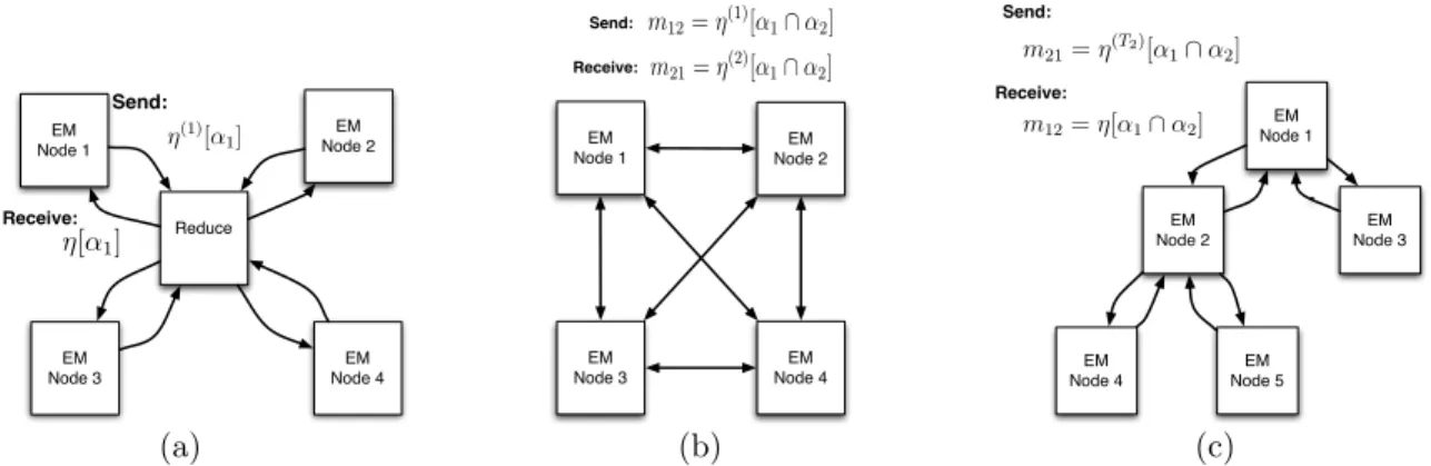
EM Node 1 EM Node 3 EM Node 4 EM Node 2 Reduce Receive: Send: η(1)_[α1] η[α1] EM Node 1 EM Node 3 EM Node 4 EM Node 2 Send: Receive: m₂₁=η(2)[α₁∩α₂] m12=η(1)[α1∩α2] EM Node 4 EM Node 3 EM Node 1 EM Node 2 EM Node 5 Receive: Send: m12=η[α1∩α2] m21=η(T2)[α1∩α2] (a) (b) (c)

Figure 3: (a)_MapReduce: Each node computes partial statistics in a local E-Step, sends these to a central “Reduce” node, and receives back completed statistics relevant for completing its local M-Step. (b)_AllPairs: Each node communicates to each other node only the relevant partial sufficient statistics. For many applications, these intersections will be small. (c)JunctionTree: The network topology is a tree, chosen heuristically to optimize any desired criteria (e.g., bandwidth). 4.1. MapReduce Topology

A straightforward way to implement the C-Step is to have each node send its non-zero partial countsη(i)[αi]

to a central “Reduce” node for accumulation into η. This central node then returns only the relevant com-pleted countsη[αi] to the nodes so that they can

inde-pendently perform their local M-Steps. This approach, depicted in figure 3(a), is roughly analogous to the topology used in the MapReduce framework (Dean & Ghemawat, 2004). When parameters are numerous, this will already be more bandwidth-efficient than a naive MapReduce approach, in which the Reduce node would perform a global M-Step and then sendallof the new parametersθ back to all nodes for the next iter-ation. To enable sending only relevant counts η[αi],

the actual iterations are preceded by a setup phase in which each node constructs an array of relevant count indices αi and sends this to the Reduce node. This

array also fixes an ordering on relevant statistics, so that later messages of counts can be densely encoded.

This _MapReduce topology3 _{may be a good choice}

for the C-Step when nodes share most of the same statistics. On the other hand, if sufficient statistics are sparse and numerous, the central reduce node can be a significant bandwidth and memory bottleneck in the distributed EM algorithm. Indeed, in practice, with either Model 1 or LDA, available amounts of train-ing data can and do easily cause the sufficient statis-tics vectors to exceed the memory of any single node.

TheMapReducetopology for estimation of LDA has

3_{For the remainder of this paper we will use}

MapRe-duceto refer to thetopologyused by the MapReduce

sys-tem (Dean & Ghemawat, 2004). While the particular de-tails of our implementation will differ substantially from the MapReduce system (e.g., we use a single reduce node), many key results should hold more generally (e.g., the MapReduce approach uses unnecessarily high bandwidth).

been discussed in related work, notably Newman et al. (2008), though they do not consider the sparse distri-bution of the M-step, which is necessary for very large data sets.

4.2. AllPairs Topology

MapReducetakes a completelycentralizedapproach

to implementing the C-Step, in which the accumula-tion ofηat the Reduce node can be slow or even infea-sible. This suggests adecentralizedapproach, in which nodes directly pass relevant counts to one another and no single node need store all of η or θ. This section describes one such approach, AllPairs, which in a sense represents the opposite extreme from

MapRe-duce. In AllPairs, the network graph is a clique

on the k nodes, and each node i passes a message

mij = η(i)[αi ∩αj] to each other node j containing

precisely the statistics j needs and nothing more (see figure 3(b)). Each nodejthen computes its completed set of sufficient statistics with a simple summation:

η[αi] =η(i)+ X j6=i mji =η(i)+X j6=i η(j)[αi∩αj]

AllPairs requires a more complicated setup phase,

where each node i calculates, for roughly half of the other nodes, the intersection αi ∩αj of its

parame-ters with the other node j’s.4 _{Node i then sends the} contents of this intersection toj.

In each iteration, message passing proceeds asyn-chronously, and each node begins its local M-Step as

4

Note that the C-Step time is now sensitive to how our data is partitioned. An interesting area for future work is intelligently partitioning the data so that data split inter-sections are small.

soon as it has finished sending and receiving the neces-sary counts. An important point is that, to avoid dou-ble counting, a received count cannot be folded into a node’s local statistics until the local copy of that count has been incorporated into all outgoing messages.

AllPairsis attractive because it lacks the bandwidth

bottleneck of _MapReduce, all paths of communica-tion are only one hop long, and each node need only be concerned with precisely those statistics relevant for its local E- and M-steps. On the down side,_AllPairs needs a full crossbar connection between nodes, and requires unnecessarily high bandwidth for dense suffi-cient statistics that are relevant to datums on many nodes. In particular, a statistic that is relevant to k0

nodes must be passedk0_(k0_{−1) times, as compared to}

an optimal value of 2(k0−1) (see section 4.3). 4.3. JunctionTree Topology

A tree-based topology related to the junction tree ap-proach used for belief propagation in graphical models (Pearl, 1988) can avoid the bandwidth bottleneck of

MapReduce and the bandwidth explosion of

All-Pairs. In this approach, theknodes are embedded in

an arbitrary tree structureT, and messages are passed along the edges in both directions (see figure 3(c)). We are certainly not the first to exploit such structures for distributing computation; see particularly Paskin et al. (2004), who use it for inference rather than estimation. We first describe the most bandwidth-efficient method for communicating partial results about asingle statis-tic, and then show how this can be extended to pro-duce an algorithm that works for the entire C-Step. Consider a single sufficient statisticηx(e.g., some ηst

for Model 1) which is only relevant to E- and M-Steps on some subset of machines S. Before the C-Step, each node hasηx(i), and after communication each node

should have ηx = Pi∈Sη

(i)

x . We cannot hope to

ac-complish this goal by passing fewer than 2(|S| −1) pairwise messages; clearly, it must take at least|S| −1 messages before any node completes its counts, and then another |S| −1 messages for each of the other |S|−1 nodes to complete theirs too. This is fewer mes-sages than either_MapReduceor_AllPairspasses. This theoretical minimum bandwidth can be achieved by embedding the nodes of S in a tree. After desig-nating an arbitrary node as the root, each node accu-mulates a partial sum from itssubtreeand then passes it up towards the root. Once the root has accumu-lated the completed sum ηx, it is recursively passed

back down the tree until all nodes have received the completed count, for a total of 2(|S| −1) messages.

Of course, each node must obtain a set of complete relevant statistics η[αi] rather than a single statistic ηx. One possibility is to pass messages for each

suffi-cient statistic on a separate tree; while this represents thebandwidth-optimalsolution for the entire C-step, in practice the overhead of managing 240 million different message trees would likely outweigh the benefits. Instead, we can simply force all statistics to share the

sameglobal treeT. In each iteration we proceed much as before, designating an arbitrary root node and pass-ing messages up and then down, except that now the message mij from node i to j conveys the

intersec-tion of their relevant statistics αi∩αj rather than a

single number. For this to work properly, we require thatThas the followingrunning intersectionproperty: for each sufficient statistic, all concerned nodes form a

connected subtreeof T. In other words, for all triples of nodes (i, x, j) where x is on the path from i to j, we must have (αi∩αj) ⊆ αx. We can assume that

this property holds, by augmenting sets of statistics at interior nodes if necessary.

When the running intersection property holds, the message contents can be expressed as

mij =η(Ti)[αi∩αj] towards root mji=η[αi∩αj] away from root

where Ti is used to represent the subtree rooted at i, and η(Ti) _{is the sum of statistics from nodes in this}

subtree. Thus, the single global message passing phase can be thought of as|α|separate single-statistic mes-sage passing operations proceeding in parallel, where the root of each such phase is the node in its sub-tree closest to the global root, and irrelevant opera-tions involving other nodes and statistics can be ig-nored. In our actual implementation, we instead use an asynchronous message-passing protocol common in probabilistic reasoning systems (Pearl, 1988), which avoids the need to designate a root node in advance. The setup phase for _JunctionTree proceeds as fol-lows: (1) All pairwise intersections of statistics are computed and saved to shared disk. (2) An arbitrary node chooses and broadcasts a directed, rooted treeT

on the nodes which optimizes some criterion. (3) Each node (except the root) constructs the set of statistics that must lie on its incoming edge, by taking the union of the intersections of statistics (which can be reread from disk) for all pairs of nodes on opposite sides of the edge.5 _{(4) Each node passes the constructed edge set} along its incoming edge, fixing future message struc-tures in the process. (5) Each node augments itsαito

5_{More efficient algorithms are possible, but they require} more memory.

include all statistics in local outgoing messages, thus enforcing the running intersection property.

To choose a heuristically good topology, we use the maximum spanning tree (MST) with edge weights equal to the sizes of the intersections|αi∩αj|, so that

nodes with more shared statistics tend to be closer to-gether. This heuristic has been successfully used in the graphical models literature (Pearl, 1988) to construct junction trees. However, in general one can imagine much better heuristics that also consider, e.g., max degree, tree diameter or underlying network structure. If statistics tend to be well-clustered within and be-tween nodes, we can expect this MST to require less bandwidth than either alternate topology, and (like

AllPairs) there should be no central bandwidth

bot-tleneck. On the other hand, if statistics tend to be shared between only a few nodes and this sharing is not appropriately clustered, bandwidth and memory may increase because many statistics will have to be added to enforce the running intersection property.6 Furthermore, if the diameter of the tree is large, la-tency may become an issue as many sequential message sending and incorporation steps will have to be per-formed. Finally, the setup phase takes longer because choosing the tree topology and enforcing the running intersection property may be expensive. Despite these potential drawbacks, we will see that MST generally performs best of the three topologies investigated here in terms of both bandwidth and total running time. As a final note, if T is a “hub and spoke” graph, and the hub’s statistics are augmented to contain all ofη, a_MapReducevariant is recovered as a special case of

JunctionTree. This is the version of MapReduce

we actually implemented; it differs from the version described in section 4.1 only in that the role of reduce node is assigned to one of the workers rather than a separate node, which reduces bandwidth usage.

5. Experiments

We performed experiments using the word alignment model from section 2.1 and the LDA topic model from section 2.2. For each of these models, we com-pared the network topologies used to perform the C-Step and how they affect the overall efficiency of EM. We implemented the following topologies (described in section 4): MapReduce, AllPairs, and

Junc-tionTree. Although our implementation was done in

Java, every reasonable care was taken to be time and memory efficient in our choice of data structures and in

6

This could be avoided by using different trees for dif-ferent sets of statistics; we leave this for future work.

network socket communication. All experiments were performed on a cluster of identical, load-free 3.0 GHz 32-bit Intel machines. Running times per iteration represent the median over 10 runs of the maximum time on any node. We also examine the bandwidth of each topology, measured by the number of counts communicated across the network per iteration. 5.1. Word Alignment Results

We performed Model 1 (see section 2.1) experiments on the UN Arabic English Parallel Text TIDES Ver-sion 2 corpus, which consists of about 3 million sen-tences of translated UN proceedings from 1994 until 2001.7 For the full data set, there are more than 243 million distinct parameters.

In table 1(a), we present results where the number of sentence-pair datums per node is held constant at 145K and the number of nodes (and thus total training data) is varied. For 10 or more nodes, the MapRe-duce topology runs out of memory due to the

num-ber of statistics that must be stored in memory at the Reduce node.8 _{In contrast, both}

AllPairs and

JunctionTreecomplete training for the full data set

distributed on 20 nodes.

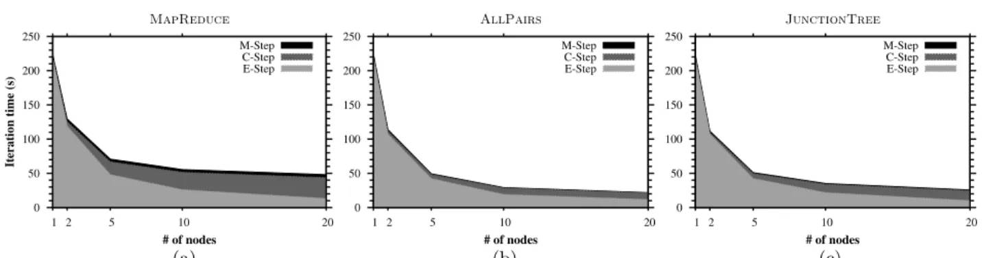
We also experimented with the setting where we fix the total amount of data at 200K sentences, but add more nodes to distribute the work. Figure 4 gives iteration times for all three topologies broken down according to E-, C-, and M-Steps. TheMapReducegraph (fig-ure 4(a)) shows that the C-Step begins dominating run time as the number of nodes increases. This effect reduces the benefit from distributing EM for larger numbers of nodes. Both _AllPairs and

Junction-Tree have substantially smaller C-Steps, which con-tributes to much faster per-iteration times and also allows larger numbers of nodes to be effective. On the full dataset,_JunctionTreeoutperforms

All-Pairs, but not by a substantial margin. Although

the two topologies have roughly comparable running times, they have different network behaviors. Figure 5, which compares bandwidth usage in billions of counts transferred over the network per iteration, shows that

AllPairsuses substantially more bandwidth than

ei-ther MapReduce or JunctionTree. This is due

to the O(k2) number of messages sent per iteration. In contrast,_JunctionTreetypically has a higher la-7_{LDC catalog #LDC2004E13. Seehttp://projects.}

ldc.upenn.edu/TIDES/index.html.

8

This issue could be sidestepped by using multiple Re-duce nodes as in the MapReRe-duce system; however, the fun-damental inefficiency of the MapReduce topology would remain.

0 50 100 150 200 250 1 2 5 10 20 Iteration time (s) # of nodes MapReduce M-Step C-Step E-Step 0 50 100 150 200 250 1 2 5 10 20 # of nodes AllPairs M-Step C-Step E-Step 0 50 100 150 200 250 1 2 5 10 20 # of nodes JunctionTree M-Step C-Step E-Step (a) (b) (c)

Figure 4: Speedup of median iteration time for three topologies as a function of the number of nodes, training Model 1 on 200k total sentence pairs. Time for each iteration is broken down into E-, C-, and M-Step time. The M-Step is present but difficult to see due to its brevity.

0 0.5 1 1.5 2 2.5 3 3.5 4 1 2 5 10 20

Bandwidth (billions of statistics)

# of nodes

Distributed Model 1 Bandwidth MapReduce

AllPairs JunctionTree Optimal

Figure 5: Bandwidth usage for three topologies compared to optimal, as a function of the number of nodes, training on Model 1 with 145k sentence pairs per node. MapRe-duceran out of memory when run on more than 5 nodes.

tency due to the fact that nodes must wait to receive messages before they can send their own. _AllPairs

andJunctionTreewith the MST heuristic represent

a bandwidth and latency tradeoff, and the choice of which to use depends on the properties of the partic-ular network.

5.2. Topic Modeling Results

We present results for the variational EM LDA topic model presented in section 2.2. Our results are on the Reuters Corpus Volume 1 (Lewis et al., 2004). This corpus consists of 804,414 newswire documents, where all tokens have been stemmed and stopwords removed.9 There are approximately 116,000 unique word types after pre-processing. The number of pa-rameters of interest is therefore 116,000T, whereT is the number of topics that we specify.

We experimented with this model on the entire corpus and varied the number of topics. The largest num-9_{We used the processed version of the corpus provided} by Lewis et al. (2004). 0 200 400 600 800 1000 1200 1400 1600 1800 0 100 200 300 400 500 600 700 800 900 1000 Iteration time (s) # of topics

Distributed LDA Iteration Time (20 nodes) MapReduce

AllPairs JunctionTree

Figure 6: Median iteration time for three topologies, as a function of the number of topics, training on LDA with 20 nodes and all 804k documents.

ber of topics we used wasT = 1,000, which yields 116 million unique parameters. Our results on iteration time are presented in figure 6. Note that the number of parameters depends linearly on the number of top-ics, which can roughly be seen in figure 6. This figure demonstrates that the efficiency of theAllPairsand

JunctionTree topologies as the number of

parame-ters increases. We see that_JunctionTreeedges out

AllPairsfor a larger number of topics.

Table 1(b) shows detailed results for the experiment depicted in figure 6. Besides the difference in itera-tion times for the three algorithms as the number of topics (and statistics) grows, there are at least two other salient points. First, while the number of to-tal statistics grows similarly to in the word alignment experiments, here the number of unique statistics is significantly smaller (i.e., each statistic, on average, is relevant to more nodes). This leads to significantly worse performance, especially in terms of bandwidth, forAllPairs. A second point is that setup times are much lower than for word alignment, because sets of relevantwordscan be determined first, and only then expanded to (word, topic) pairs.

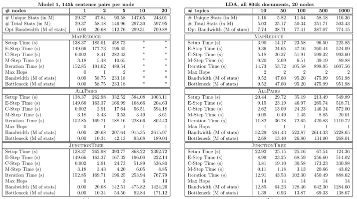
Model 1, 145k sentence pairs per node LDA, all 804k documents, 20 nodes

# nodes 1 2 5 10 20

# Unique Stats (in M) 29.37 47.84 90.58 147.65 243.01 # Total Stats (in M) 29.37 58.18 146.96 297.30 597.95 Opt Bandwidth (M of stats) 0.00 20.68 112.76 299.31 709.88

MapReduce Setup Time (s) 138.37 185.01 458.72 * * E-Step Time (s) 149.66 177.73 196.45 * * C-Step Time (s) 0.002 8.41 282.43 * * M-Step Time (s) 3.18 5.48 10.65 * * Iteration Time (s) 152.85 191.62 489.54 * * Max Hops 0 1 2 * * Bandwidth (M of stats) 0.00 58.75 233.18 * * Bottleneck (M of stats) 0.00 58.75 233.18 * * AllPairs Setup Time (s) 138.37 262.98 332.52 584.08 1003.11 E-Step Time (s) 149.66 163.37 166.99 168.66 204.63 C-Step Time (s) 0.002 2.91 17.64 56.51 594.18 M-Step Time (s) 3.18 3.43 3.53 3.49 3.61 Iteration Time (s) 152.85 169.71 188.16 228.66 802.43 Max Hops 0 1 1 1 1 Bandwidth (M of stats) 0.00 20.68 207.64 915.35 3615.97 Bottleneck (M of stats) 0.00 10.34 42.13 93.68 189.04 JunctionTree Setup Time (s) 138.37 262.98 393.77 868.22 2392.72 E-Step Time (s) 149.66 163.37 167.32 196.00 222.14 C-Step Time (s) 0.002 2.91 24.73 51.89 536.80 M-Step Time (s) 3.18 3.43 4.20 6.05 8.85 Iteration Time (s) 152.85 169.71 196.25 253.94 767.79 Max Hops 0 1 3 6 13 Bandwidth (M of stats) 0.00 20.68 142.51 475.82 1424.26 Bottleneck (M of stats) 0.00 10.34 54.50 92.84 171.12 # topics 10 50 100 500 1000

# Unique Stats (in M) 1.16 5.82 11.64 58.18 116.36 # Total Stats (in M) 5.03 25.17 50.34 251.71 503.43 Opt Bandwidth (M of stats) 7.74 38.71 77.41 387.07 774.15

MapReduce Setup Time (s) 3.90 14.17 23.58 96.50 225.85 E-Step Time (s) 9.36 24.65 47.16 260.44 524.09 C-Step Time (s) 5.18 26.37 51.91 599.32 993.60 M-Step Time (s) 0.20 2.69 6.51 39.19 89.88 Iteration Time (s) 14.73 53.72 105.58 898.95 1607.56 Max Hops 2 2 2 2 2 Bandwidth (M of stats) 9.52 47.60 95.20 475.99 951.98 Bottleneck (M of stats) 9.52 47.60 95.20 475.99 951.98 AllPairs Setup Time (s) 20.44 29.72 35.19 213.49 549.89 E-Step Time (s) 9.15 23.19 46.97 265.74 518.71 C-Step Time (s) 2.62 13.09 24.23 146.24 572.00 M-Step Time (s) 0.05 0.49 1.45 8.85 20.01 Iteration Time (s) 11.82 36.78 72.65 420.83 1110.72 Max Hops 1 1 1 1 1 Bandwidth (M of stats) 52.29 261.43 522.87 2614.33 5228.65 Bottleneck (M of stats) 2.68 13.40 26.80 134.00 268.01 JunctionTree Setup Time (s) 22.92 25.15 25.16 67.54 124.36 E-Step Time (s) 8.99 23.25 68.59 256.60 514.02 C-Step Time (s) 3.81 19.10 30.58 173.23 330.98 M-Step Time (s) 0.11 1.18 3.13 20.66 43.62 Iteration Time (s) 12.91 43.53 102.30 450.49 888.62 Max Hops 14 14 14 14 14 Bandwidth (M of stats) 12.85 64.23 128.46 642.30 1284.60 Bottleneck (M of stats) 1.39 6.93 13.87 69.33 138.67 (a) (b)

Table 1: (a) Results for scaling up number of nodes, training Model 1 with 145k sentence pairs per node. (b) Results for scaling up number of topics, training LDA with all 804k documents on 20 nodes. All times are measured in seconds, statistics are counted in millions, and bandwidths are measured in millions of statistics passed per iteration. # unique stats measures|α|, whereas # total stats measuresP

i|αi|. Opt bandwidth is theoretically optimal bandwidth (see section 4.3). Setup time includes all time until all nodes started the first E-Step. Median total time per iteration is given, as well as a breakdown into E-, C-, and M-Steps. Max hops is the diameter of the graph. Bottleneck is maximum bandwidth in and out of any single node. (*) indicates an out-of-memory error.

We note that the total bandwidth is actually lower

forMapReducethanJunctionTreesince the MST

only heuristically minimizes the number of discon-nected statistic components, rather than the true cost of enforcing the running intersection property. Despite this, the bandwidth bottleneck for _JunctionTreeis still much lower than forMapReduce.

6. Conclusion

We have demonstrated theoretically and empirically that a distributed EM system can function success-fully, allowing for both significant speedup and scaling up to computations that would be too large to fit in the memory of a single machine. Future work will con-sider applications to other machine learning methods, alternative junction tree heuristics, and more general graph topologies.

Acknowledgments

The authors of this work were supported (respectively) by DARPA IPTO contract FA8750-05-2-0249, a Mi-crosoft Research Fellowship, and a MiMi-crosoft Research New Faculty Fellowship.

References

Blei, D. M., Ng, A. Y., & Jordan, M. I. (2003). Latent Dirichlet Allocation. JMLR,3, 993–1022.

Brown, P. F., Pietra, S. D., Pietra, V. J. D., & Mercer, R. L. (1994). The Mathematics of Statistical Machine Translation: Parameter Estimation.Computational Lin-guistics,19, 263–311.

Chu, C.-T., Kim, S. K., Lin, Y.-A., Yu, Y., Bradski, G., Ng, A. Y., & Olukotum, K. (2006). Map-Reduce for Machine Learning on Multicore. NIPS.

Dean, J., & Ghemawat, S. (2004). MapReduce: Simplified Data Processing on Large Clusters.Sixth Symposium on Operating System Design and Implementation.

Dempster, A. P., Laird, N. M., & Rubin, D. B. (1977). Maximum Likelihood from Incomplete Data via the EM Algorithm. Journal of the Royal Statistical Society. Lewis, D. D., Yang, Y., Rose, T. G., & Li, F. (2004). RCV1:

A New Benchmark Collection for Text Categorization Research. JMLR.

Newman, D., Asuncion, A., Smyth, P., & Welling, M. (2008). Distributed Inference for Latent Dirichlet Al-location. NIPS.

Nowak, R. (2003). Distributed EM algorithms for den-sity estimation and clustering in sensor networks. IEEE Transactions on Signal Processing,51, 2245–2253. Paskin, M., Guestrin, C., & McFadden, J. (2004). Robust

Probabilistic Inference in Distributed Systems. UAI. Pearl, J. (1988). Probabilistic Reasoning in Intelligent