Calculation of Bit Error Rates in Optical Fiber Communications Systems in the Presence of Nonlinear Distortion and Noise. by Oleg V.

(1)

Calculation of Bit Error Rates in Optical Fiber

Communications Systems in the Presence of

Nonlinear Distortion and Noise

by

Oleg V. Sinkin

Dissertation submitted to the Faculty of the Graduate School

of the University of Maryland in partial fulllment

of the requirements for the degree of

Doctor of Philosophy

(2)

LIST OF FIGURES

1.1 Pattern dependent nonlinear eect in a WDM RZ system. . . 3 2.1 Simple communications system. Reproduced from [149] . . . 8 2.2 Dispersion slope characteristics of two ber pairs . . . 15 2.3 RZ eye diagrams with (a) suboptimal and (b) optimal pre- and

post-compensation with the corresponding accumulated dispersion functions. 17 2.4 Timing jitter as a function of distance. . . 18 2.5 Eye opening as a function of average map dispersion. . . 21 3.1 Plot of the total number of FFTs versus global relative error ε for

second-order (a) and fth-order (b) solitons. . . 33 3.2 Plot of the total number of FFTs versus global relative error ε for a

collision of two rst-order solitons. . . 34 3.3 Step size has a function of distance for the local error method applied

to a collision of two rst-order solitons. . . 34 3.4 Plot of the total number of FFTs versus global relative error ε for the

single-channel (a) DMS and (b) CRZ systems. . . 37 3.5 Plot of the total number of FFTs versus global relative error ε _{for the}

(5)

3.6 Step size has a function of distance for the local-error method applied to the multichannel CRZ system. The upper two plots show the step sizes for the rst two and last two periods of the dispersion map, and the lower two plots show the corresponding portions of the dispersion

map. Triangles indicate the positions of ampliers. . . 40

3.7 Plot of the global error as a function of method parameter for (a) local error, (b) walk-o, (c) nonlinear phase, (d) logarithmic step, and (e) constant step methods. . . 41

5.1 Time shift function for two pump channels. . . 75

5.2 Collision dynamics for three dierent pulses. . . 76

5.3 The scaled time shift function. . . 77

5.4 Worst-case time shift vs. number of channels N. . . 79

5.5 Probability density function of the collision-induced time shift. . . . 85

6.1 Conversion of time shift to the current distortion. . . 89

6.2 Probability density function of the current due to the nonlinear distor-tions with a single pulse in the target channel. . . 91

6.3 Probability density function of the current at the detection point in the receiver due to the nonlinear distortion with multiple pulses (MP) in the target channel compared to a single pulse in the target channel (SP). . . 94

6.4 Pdf of the current in marks and spaces at the decision time due to the nonlinear distortions and noise obtained using (6.38). . . 103

(6)

LIST OF TABLES

2.1 Characteristics of D+/D− and SMF/DCF ber pairs. . . 14

(7)

1. INTRODUCTION

A fundamental goal of modeling ber communications systems is to understand the physics of the system behavior and to develop computational tools to design sys-tems and predict their performance. Transmission of data through a ber-optic link unavoidably leads to bit errors due to various eects, the dominant of which are noise from optical ampliers, ber nonlinearity, polarization eects, and non-ideal transmitters and receivers. There exist numerous studies that provide techniques to characterize all of these eects and to calculate the bit error ratio (BER) due to them [1][4]. However, there are still many important unanswered questions and one of them is how to accurately calculate the bit error ratio (BER) in the presence of nonlinear signal distortion.

Why is a careful analysis of nonlinear eects in optical ber communications systems important? Nearly all modern systems operate in the linear propagation regime, in which the signal evolution is almost linear [5]. However, there always ex-ist small nonlinear interactions and small nonlinear signal dex-istortions accumulated during transmission over hundreds and thousands of kilometers can lead to an in-crease in the error rate. Reducing the optical power dein-creases the importance of the nonlinear interactions, but it also decreases the signal-to-noise ratio. There exists an optimal power level at which the BER is minimal. Even if the power level is much lower than optimum, the accumulation of nonlinear distortions during transmission over hundreds or thousands of kilometers of ber can introduce a signicant system penalty [6][9]. Calculating the BER in such a regime or nding the optimal power level requires an accurate model of the nonlinear interactions.

(8)

The main challenge in characterizing the nonlinear penalty is that it is a statistical quantity. In on-o keyed systems, a digital 1 (mark) is represented by the presence of an optical pulse and a digital 0 (space) is represented by its absence. The amount of distortion that an optical pulse suers depends on the particular pattern of surround-ing pulses, which is eectively random as these pulses represent the information bits, and the information sequence of bits is quasi-random. This eect is often referred to as the nonlinear pattern-dependence eect [1], [10]. In single-channel transmis-sion, dispersion leads to the spread of optical signals, causing approximately three to seven adjacent pulses to interfere [5], [11]. Therefore, a common approach to account for pattern-dependent nonlinear eects is to use a pseudo-random sequence of bits, which is typically 23₋₂7 _{bits, to nd the worst-case bit in the sequence. When we}

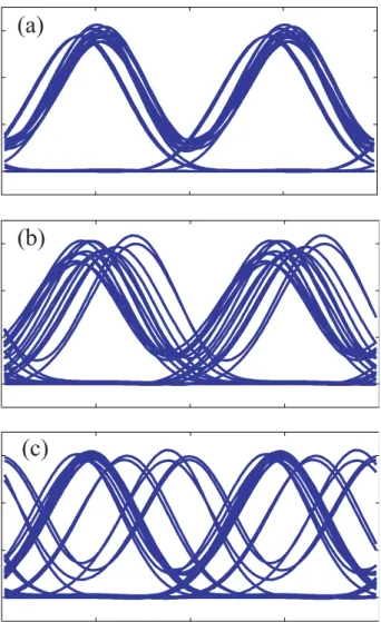
consider a multi-channel system, this approach is inappropriate since there are many more pulses interacting with each other due to the dispersive walko between the fre-quency channels. As an illustration, Fig. 1.1 shows three simulated eye diagrams of a noise-free signal in the center channel of a 10 Gb/s wavelength-division multiplexed (WDM) return-to-zero (RZ) system after propagating over 5000 km. We used nine co-polarized channels spaced by 50 GHz and the average power was approximately −0.7_{dBm per channel. We used three dierent sets of bit patterns in dierent WDM}

channels, while the bit pattern in the center channel remained unchanged. As we move from 1.1a to 1.1c, it is apparent that the eye changes from being almost com-pletely open to comcom-pletely closed. In this case, nding the worst-case performance becomes not only prohibitively time-consuming since the number of possible inter-action patterns grows exponentially, but it is also not useful because the likelihood of the worst-case pattern is negligibly small. Therefore, a probabilistic approach is necessary to treat this problem.

Typically, the dominant nonlinear eect in modern high-speed systems operating at 10 GB/s, is cross-phase modulation [7], [8], [12][15]. The phase of an optical

(9)

(a)

(b)

(c)

Fig. 1.1: Pattern dependent nonlinear eect in a WDM RZ system.

pulse is changed by the presence of pulses in either the same or neighboring wave-length channels. This phase change leads to intensity distortion by means of ber dispersion. The manifestation of this eect depends on the light modulation format. In non-return-to-zero (NRZ) transmission, the signal distortion appears in the form of amplitude jitter [14], [16][18], while in the RZ systems, the dominant nonlinear eect is typically collision-induced timing-jitter [12], [19][23]. This fact requires the development of completely dierent approaches to account for the nonlinear eects in these two types of systems. We note that at present, the NRZ and RZ modulation formats are still the most commonly used formats in optical ber communications systems. The NRZ format is the simplest form of intensity modulation and it has

(10)

been historically the format of choice for many system providers. Recently, it has been discovered that the RZ-modulated signal undergoes less intersymbol interfer-ence in the receiver and is more robust to ber nonlinearities and thus more capable of long-haul data transmission [11], [22], [24][27]. Because the NRZ modulation has been used for many years, techniques have been developed to characterize the nonlinear eects in WDM NRZ transmission [14], [16][18], [28][36], and the BER calculations based on these techniques agree well with experimental results. The basic idea in these approaches [16], [30][32] is to utilize a pump-probe method, in which the cross-phase modulation-induced distortion is treated as an additive perturbation. An exception is [36] where the authors treat the distortion as multiplicative. In order to determine the inuence of the nonlinearity on the system performance, one further assumes that the XPM-induced distortion may be treated as additive Gaussian noise and a correction to the Q-factor is calculated [14], [16], [30], [33][35], [37].

The major nonlinear eect in WDM RZ systems, collision-induced timing jitter, has also been well studied in both soliton and linear systems [12], [19][21], [38][44]. It is well known how to calculate the time shift that results from a collision of a pair of pulses and to calculate the standard deviation of the time shift. However, no accurate BER calculation that takes into account the inter-channel nonlinear bit-pattern eect due to this timing jitter has been reported in the literature.

The purpose of this dissertation research is to develop a method that allows one to accurately account for inter-channel nonlinear crosstalk in calculations of BER in WDM return-to-zero systems.

Our method of computing the BER in the presence of the nonlinear distortion and amplied spontaneous emission noise, is based on calculations of the complete probability density function (pdf) of the nonlinearly-induced amplitude or timing jitter. Using the knowledge of the pdf of the noise-induced amplitude variation, we combine the noise and nonlinear contributions to calculate the resulting BER.

(11)

The dissertation is organized as follows:

In the second chapter, we describe a prototypical undersea system to which we apply our BER calculation technique. We discuss some system design tradeos and the performance optimization issues.

In the third chapter, we review commonly used methods used to characterize the eects of ber nonlinearity in optical ber communications systems.

The fourth chapter contains a summary and discussion of the biased Monte Carlo methods that can be used to estimate the pdf of the received current or the time shift of a pulse for the values of the pdf ranging over many orders of magnitude.

In the fth chapter, we introduce the time shift function, a function that describes the time shift of a pulse in a two-pulse collision, depending on the frequency and initial time separation of the two pulses. We discuss the properties of the time shift function and use it to calculate the pdf of the collision-induced time shift by means of the characteristic function method. Finally, we validate this method of computing the pdf of the time shift with biased Monte Carlo simulations.

In the sixth chapter, we present and validate a method for evaluating the pdf of the received current due to nonlinear eects in transmission. Then, we describe an additive white Gaussian noise model for calculating the pdf of the received current and show how to calculate the BER using the methods that we presented.

The seventh chapter contains the conclusions that summarize the main results of the dissertation.

(12)

2. TEST SYSTEM

In this chapter, we present a prototypical long-haul undersea system that uses WDM technology and an RZ modulation format. Long-haul submarine transmission sys-tems represent a signicant and rapidly growing portion of the world ber optic net-work [45] and a large portion of current transoceanic transmission lines operate using the RZ modulation format, including cable systems built by Tyco Telecommunica-tions, Marconi, NEC Submarine Systems, and Fujitsu. These systems typically have shorter values of amplier spacing and longer transmission distances than terrestrial systems. The propagation length in these systems is limited by the tradeo between the signal-to-noise ratio and the accumulation of the nonlinear penalties. Hence it is especially important to develop accurate tools to model nonlinear impairments for these types of systems.

The original goal of this dissertation was to perform a comparative study of spec-tral eciency of dierent modulation formats. In order to do this, we had to optimize system parameters for each format and dierent values of channel spacing. In particu-lar, for a given channel spacing we varied the average map dispersion and the pre- and post-compensation to determine the optimal dispersion prole for each modulation format. During the initial study, we encountered the nonlinear pattern-dependence eect [1], [10]. Exploration of this matter led us to a more general, and, in our view, more important research topic. The current goal of this dissertation is to develop new and accurate tools to evaluate the eect of ber nonlinearity on the performance of RZ systems. In this chapter, we describe only the RZ system that we used to develop our methodology, and we summarize the optimization of the dispersion prole for this

(13)

(14)

2.1 System model

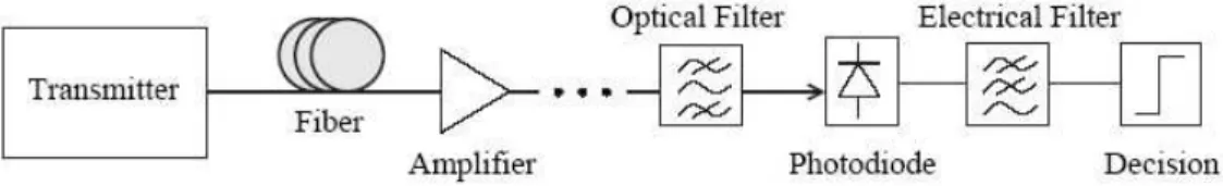
Typical modern ber communications systems contain a large number of optical com-ponents such as lasers, modulators and demodulators, multiplexers and demultiplex-ers, ltdemultiplex-ers, optical bdemultiplex-ers, and ampliers [1], [2]. In addition, there is an extensive set of electrical equipment at the receiver, such as photodiodes, electrical lters, ampli-ers, and decision circuits. When simulating these components, the level of detail of the model must be appropriate for the system under study. For example, a lumped amplier model is used often for optical ampliers, in which the optical eld is simply multiplied by a factor. We use this model in the simulations in this dissertation. More realistic models can include amplied spontaneous emission noise, gain satura-tion, the gain prole, polarization hole burning, and transients [46]. The rst step of any simulation is to simplify the system and to restrict the model of the optical propagation to the essential eects. The nature of the most important eects strongly depends on the type of the optical system. In particular, the amount of nonlinearity has an important impact on the evolution of the signal and the noise.

Figure 2.1 shows a schematic illustration of a simple model of an optical ber com-munications system that is used in this dissertation. The optical signal is generated by a transmitter and inserted into the ber. It then passes through a transmission line that primarily consists of ber spans and optical ampliers. At the end of the transmission line, the signal is optically ltered and enters a receiver, where it is converted to an electrical current by a high-speed photodiode. This current passes

(15)

through a low-pass lter and enters a decision circuit.

In a typical digital optical ber transmission system, the pulses are either directly created by an optical laser, or the output of a constant wave laser is modulated by an external modulator. We will only discuss on-o keying in this dissertation. In RZ transmission, the marks are represented by isolated optical pulses, while in NRZ signaling, a sequence of marks is represented by a continuous constant light intensity. We assume that the amplitude modulation is produced by a Mach-Zehnder interferometer. The functional form of the RZ or chirped-RZ (CRZ) complex eld envelope that is used in this dissertation is

U(t) = r 1 2 h 1 + cos ³ πsinπt T ´i exp ³ iCπcos2πt T ´ , (2.1)

where T is the bit period and C is the chirp parameter [11], [47]. The parameter C equals zero for the unchirped RZ signal. The pulse stream may then be combined with pulse streams with dierent central frequencies to make a single WDM signal [1], [2]. In this work, we used nine co-polarized WDM channels, spaced by 50 GHz, each carrying a 10-GB/s unchirped RZ signal. We used dierent values of peak power in the system optimization step; however, we set the peak power to 5 mW per channel in the rest of the study.

Transmission of light through optical ber can be described by the nonlinear Schrödinger (NLS) equation [48] ∂u(z, t) ∂z +i β00₍_z₎ 2 ∂2_u₍_{z, t}₎ ∂t2 −iγ|u(z, t)| 2_u₍_{z, t}_{) =} _g₍_z₎_u₍_{z, t}₎_, _(2.2)

whereu(z, t) is the electric eld envelope,z is the physical distance, t is the retarded time with respect to the central frequency of the signal, β00 _{is the local dispersion,} _γ

is the Kerr coecient, and g(z) _{is the ber loss and gain coecient. This form of}

(16)

Fourier transform pairs are dened as x(t) = 1 2π Z _∞ −∞ ˜ X(ω) exp(−iωt)dω, X˜(ω) = Z _∞ −∞ x(t) exp(iωt)dt. (2.3)

This convention is common in the physics literature, but electrical engineers and mathematicians typically use the opposite convention. The literature on optical com-munications is mixed and it is not uncommon to nd work in which authors switch from one convention to the other without making any note of it. While this issue is usually not important, it can sometimes lead to errors. The implications of the dierent carrier conventions is thoroughly discussed in [49], [50]. We note as well that (2.2) does not include polarization eects. In practice, polarization eects are important because it is common to use orthogonal polarization between neighboring channels or even neighboring bits to reduce the eects of nonlinearity [8], [11], [51]. We do not take these eects into account here because they have no impact on the techniques that we present and would complicate the discussion.

The receiver subsystem includes an optical demultiplexer, square-law photode-tector, and a low-pass electrical lter as shown in Fig. 2.1. The photodetector is modeled as an ideal square-law detector without noise. We choose the spectral trans-mission function of the optical demultiplexer to be third-order super-Gaussian, where a super-Gaussian function of m-th order is dened as exp(−x2m₎_{. The bandwidth of}

the optical lter was optimized to maximize the eye opening after demultiplexing a WDM signal back-to-back and it is found to be 35 GHz for the channel spacing of 50 GHz and the unchirped RZ signal. The electrical lter is a fth-order Bessel lter, which is a typical lter in modern optical ber communications systems, and its 3-dB bandwidth is set to 8 GHz.

Finally, the decision and clock recovery circuit in this work is modeled by simply calculating the central time of a pulse at the receiver in a given channel. Since

(17)

the time reference frame is moving with the group velocity of the center channel, the pulses in the center channel do not move in this time frame due to dispersion. For pulses in other frequency channels, one can analytically account for the group delay corresponding to the particular channel. We chose this model of clock recovery because it is simple and insensitive to nonlinear distortions, which enables us to obtain a reliable estimate of the system performance. A more realistic model of the clock recovery is based on calculating the phase of one of the strong frequency components of the signal at the receiver [52], [53].

In this chapter, we discuss some aspects of system design and optimization of system parameters. For the purpose of parameter optimization, we take the eye opening at the clock recovery time as a measure of the system performance, which is dened as the dierence between the average current of a mark and the average current of a space at the detection time in the receiver.

Calculations of the eye opening are complicated by the eect of pattern-dependence during transmission due to nonlinear interactions. In a single channel system, each bit only interacts with its neighbors. All bit patterns of lengthnare contained in a de Bruijn pseudo-random bit sequence (PRBS) of lengthN = 2n_{[54]. If we increase the}

length of the PRBS, the rails of the eye diagram converge. In other words, there is a certain number of surrounding bits, n, that aect the center bit, which is determined by the amount of pulse stretching due to dispersion during transmission. Hence if we consider a PRBS of length N = 2n _{or larger, we will include all possible interaction}

patterns that may occur in any data stream in a single-channel system.

The situation becomes much more complicated when we add WDM channels to the system. In addition to interacting with a limited number of neighboring bits in the same channel, a single bit will also interact with many bits in the neighboring channels. For a xed bit string in the center channel, the resulting eye diagram, will depend on both the bit strings in the adjacent channels and the relative positions of these bit

(18)

strings. The consequence of this eect was illustrated in Fig. 1.1. An exact treatment of this problem requires a probabilistic approach, in which all possible bit patterns in the neighboring channels are considered. In order to nd a set of system parameters that optimize the performance, we run a large number of simulations, in which we keep the bit string in the center channel xed and we randomly vary the bit strings in the side channels. We compute the average eye opening from these simulations. While it is not possible to accurately infer a BER from this procedure, it is possible to reliably infer the system parameters that will produce the best performance.

(19)

2.2 Dispersion map design

All recently deployed systems employ dispersion management, in which the dispersion varies periodically. Each period consists of a concatenation of several ber spans with dierent local ber dispersions, and the variation of dispersion in one period is referred to as the dispersion map. The dispersion map is characterized by the average map dispersion D_map. For a map consisting of two ber links, D_map given by

D_map = D1L1+D2L2

L1+L2

, _(2.4)

where D1 and D2 are dispersion of the rst and the second sections of the map and

L1 and L2 are the corresponding ber lengths. The dispersion parameter D is in the

units of ps/nmkm, which is commonly used in optical communications. It is related to the second-order dispersionβ00 _{in the units of ps/km}2 _{used in (2.2) by the relation}

D=−2πc λ2 β

00_. _(2.5)

If D_map 6= 0 then the residual accumulated dispersion is compensated at the terminals by means of extra links of ber known as pre- and post-compensation bers [11], [47], [55][59]. It is typically benecial to operate the system at non-zero average dispersion. Using dispersion pre-compensation results in spreading out the optical pulses initially, which reduces the eects of four-wave mixing and cross-phase modulation [11], [22], [25]. However, excessive spreading leads to intra-channel four-wave mixing [60]. This tradeo determines the optimal value of D_map, which we will discuss further in this section. The amount of both the pre- and post-compensation dispersion must be carefully chosen as an improper choice may result in substantial intra-channel cross-phase modulation [47], [58], [61], [62].

(20)

2.2.1 Dispersion slope-matched ber pair

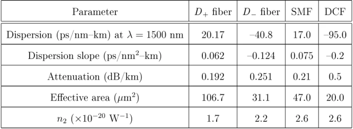
An important milestone in the development of optical ber communications systems was the introduction of dispersion-sloped matched bers [63], [64], which allowed an increase in the reach of the systems and a decrease in the cost of the terminal equipment. Dispersion slope compensation has become a key technology for both 10 and 40 Gb/s WDM systems [51], [59], [65][67]. In this work, we study a system based on dispersion slope matched bers [63], [64], often called D+ and D− bers,

whose characteristics are shown in Table 2.1. The ber transmission link is based on a dispersion map of length L, in which the rst two-thirds consist of D+ ber and

the remaining one-third consists of D− ber. The exact proportion is determined by

the desired map average dispersion, D_map = (D+L++D−L−)/L, where L+ and L−

are the lengths of the D+ and D− bers respectively.

Parameter D+ ber D− ber SMF DCF

Dispersion (ps/nmkm) atλ = 1500_nm _20.17 _40.8 _{17.0 95.0}

Dispersion slope (ps/nm2_km) _0.062 _0.124 _{0.075 0.2}

Attenuation (dB/km) 0.192 0.251 0.21 0.5 Eective area (µm2₎ _106.7 _31.1 _47.0 _20.0

n2 (×10−20 W−1) 1.7 2.2 2.6 2.6

Tab. 2.1: Characteristics of D+/D−and SMF/DCF ber

pairs.

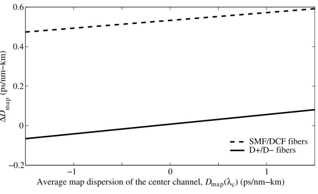
The main advantage of the D+/D− pair is that the average dispersion slope is

much smaller than when an SMF/DCF pair is used. We demonstrate this feature in Fig. 2.2. The horizontal axis represents the average map dispersion D_map(λc) of

the center channel located at λc =1550 nm. The vertical axis shows the dierence

(21)

−1 0 1 −0.2 0 0.2 0.4 0.6

Average map dispersion of the center channel, Dma p(λc) (ps/nm−km)

∆ D m a p (ps/nm−km) SMF/DCF fibers D+/D− fibers

Fig. 2.2: Dispersion slope characteristics of two ber pairs

∆D_map = |D_map(λe)−Dmap(λc)|. In this case, 2|λc −λe| = 32 nm, which

corre-spond to a WDM signal with 40 channels spaced by 100 GHz. In the case of D+/D−

bers, the variation in the average map dispersion of the center channel is very small and does not exceed a few percent. Consequently, all channels experience almost the same average map dispersion. By contrast, the SMF/DCF pair exhibits a strong wavelength dependence of the average map dispersion. For all values ofD_map(λc), the

side channels will have an average map dispersionD_map(λe) that diers from that of

the center channel by 0.40.5 ps/nmkm. For this reason it is useless to optimize the map's average dispersion for the SMF/DCF ber pair since dierent wavelengths will have completely dierent average dispersions. By contrast, using D+/D− ber pair

one may optimize the average map dispersion for WDM transmission. Other signif-icant advantages of D+/D− bers include reduced nonlinearity due to an increased

(22)

2.2.2 Optimization of dispersion prole

To optimize the dispersion prole, we considered a noiseless transmission model, based on the NLS equation (2.2), which allows us to separate the eects of nonlinearity and dispersion from the eects of the signal-noise interaction. The measure of perfor-mance was the eye opening of the optical signal in the center channel at the end of transmission.

We consider a system with a propagation distance of 5000 km and an amplier spacing of 50 km. The dispersion map consists of 34 km of D+ber and approximately

16 km of D−ber followed by an amplier. This layout is typical for modern undersea

systems [11], [51]. Since the eective nonlinearity of the D− ber is larger than that

of the D+ ber, the amplier is placed after the D− ber. Thus the signal power

at the input of the D− ber is low, which reduces the nonlinear impairments in the

system.

Optimization of dispersion pre- and post-compensation

The nonlinear interactions during transmission result in two major types of signal distortion: amplitude and timing jitter. These eects originate both from intra-channel and inter-intra-channel interactions [10]. With properly selected pre- and post-compensation one can signicantly improve the transmission quality [11], [24], [57], [58], [61]. The physical principle behind this improvement is as follows: Phase ulation induced by the nonlinear pulse interactions is converted into amplitude mod-ulation by dispersion; this amplitude modmod-ulation then causes waveform distortion. By adjusting the amount of dispersion pre-compensation and total dispersion of the transmission line this amplitude modulation can be partially reversed [37]. It has been shown that the best dispersion-compensation scheme is nearly symmetric [11], [58], [61]. Timing jitter reduction can be explained as follows: If we consider a simplied situation, in which only two pulses interact with each other [58], one can show that

(23)

the nonlinear interactions induce opposite frequency shifts for the two pulses. Due to the dispersion, these frequency shifts translate into time shifts. The magnitude of the time shifts is proportional to the dispersion and the magnitude of the frequency shift. If the accumulated dispersion is a symmetric function of distance, it changes its sign in the middle of the transmission. Hence the time shifts change their direc-tion, and the resulting timing jitter is thus canceled at the end of the transmission line. However, in realistic systems the optimum accumulated dispersion function is not perfectly symmetric and nonzero residual dispersion is often preferable, due to self-phase modulation and to the non-constant power prole.

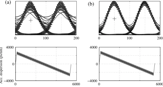
In this work, we optimize the compensation scheme by numerically nding the one that results in the maximum eye opening. In order to do so, we use single-channel transmission, so that we are only minimizing the intra-channel nonlinear eects. We x all the system parameters except for the amount of pre- and post-compensation, and we automatically adjust this amount to achieve the maximum optical eye opening. Figure 2.3 illustrates the improvement that is achieved by optimizing the dispersion

0 100 200 0 100 200 0 6000 −4000 0 4000 Acc. dispersion (ps/nm) −4000₀ ₆₀₀₀ 0 4000

(a)

_(b)

Fig. 2.3: RZ eye diagrams with (a) suboptimal and (b) optimal pre- and post-compensation with the corresponding accumulated dispersion functions.

(24)

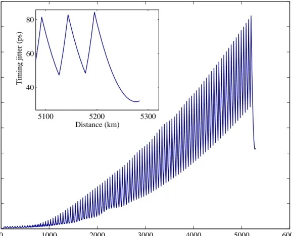
compensation scheme for our test system. We have consistently found in numerical simulations that the accumulated dispersion is a nearly symmetric function of distance and that a positive amount of residual dispersion is required to compensate for self-phase-modulation-induced distortions. We see from Fig. 2.3 that undercompensated dispersion results in an eye closure penalty. These results are consistent with previous studies [11], [24], [57], [58], [61]. 0 1000 2000 3000 4000 5000 6000 0 10 20 30 40 50 60 70 80 90 Distance (km) Timing jitter (ps) 5100 5200 5300 40 60 80 Distance (km) Timing jitter (ps)

Fig. 2.4: Timing jitter as a function of distance.

We note that we performed optimization of the pre- and post-compensation only for a single channel system. However, our recent results indicate that when we add WDM channels to this system, the optimum compensation we found for the single-channel case also results in minimizing inter-single-channel collision-induced timing jitter. Figure 2.4 shows the timing jitter, which is the standard deviation of collision-induced

(25)

time shift as a function of transmission distance. The minimum of the timing jitter occurs right at the end of the transmission, as shown in the inset, indicating that the previous choice of the pre-and post-compensation is optimum in the WDM case as well. This eect is due to the symmetry of the dispersion function, since time shifts induced in the rst and the second half of the transmission tend to cancel out.

Optimization of average map dispersion

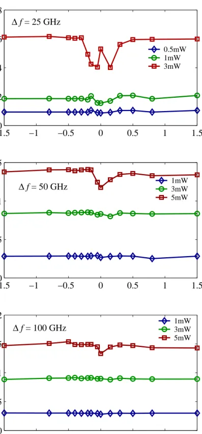
The purpose of this part of the study was to nd the optimal average map dispersion for a given value of channel spacing. The measure of performance is the optical eye opening in the center channel, which we compute as a function of the average map dispersion for dierent power levels and channel spacings. Note that for each simulation, we optimized the dispersion pre- and post-compensation for the center channel.

Figure 2.5 summarizes the results of the average map dispersion study. The dif-ferent curves in each subplot correspond to dierent power levels of the signal and dierent subplots represent the results for the channel spacing values of 25, 50, and 100 GHz. All curves have a minimum around D_map = 0, but, for the lowest input power level (diamonds), the minimum is less deep because the nonlinear interactions become weaker with a lower signal power. We also see that the range of the optimal map dispersion is large spanning from 1 to 0.3 ps/nm/km and variation in eye opening in this range are small. Existence of the optimum range of map dispersion values is explained by the tradeo between the intra- and inter-channel nonlinear interactions. For large values of dispersion, the adjacent channels slide through each other faster, thus reducing inter-channel crosstalk. However, large values of disper-sion cause a larger number of bits within one channel to overlap, resulting in an increase in the intra-channel distortion. When the total map dispersion is close to zero, intra-channel eects are weak, and the inter-channel crosstalk dominates the

(26)

eye closure [10]. Note that some of the curves are not smooth, which is attributed to inter-channel pattern eects.

For all channel spacings, the results are qualitatively the same: If the average map dispersion is close to zero, the system performance is substantially worse for all three channel spacings, but this eect is more noticeable for systems with smaller channel spacing, since the inter-channel interactions increase when the channel spacing is decreased [10]. Moreover, as the channel spacing decreases, the absolute values of optimum map dispersion increase.

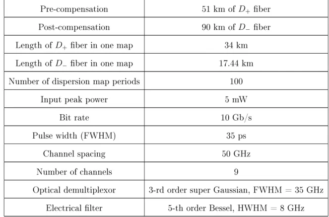
The dispersion map parameters and other system data that we used in this work are summarized in Table 2.2.

Pre-compensation 51 km of D+ ber

Post-compensation 90 km of D− ber

Length of D+ ber in one map 34 km

Length of D− ber in one map 17.44 km

Number of dispersion map periods 100

Input peak power 5 mW

Bit rate 10 Gb/s

Pulse width (FWHM) 35 ps

Channel spacing 50 GHz

Number of channels 9

Optical demultiplexor 3-rd order super Gaussian, FWHM = 35 GHz Electrical lter 5-th order Bessel, HWHM = 8 GHz

(27)

−1.50 −1 −0.5 0 0.5 1 1.5 0.2 0.4 0.6 0.8 −1.50 −1 −0.5 0 0.5 1 1.5 0.5 1 1.5 −1.50 −1 −0.5 0 0.5 1 1.5 0.5 1 1.5 2

Average map dispersion (ps/nm−km)

E y e o pening (a.u .) 1mW 3mW 5mW 1mW 3mW 5mW 0.5mW 1mW 3mW ∆f = 25 GHz ∆f = 50 GHz ∆f = 100 GHz E y e opening (a. u.) E y e opening (a. u.)

(28)

3. MODELING THE EFFECTS OF FIBER NONLINEARITY IN

OPTICAL COMMUNICATIONS

In this chapter we discuss commonly-used techniques to model the eect of ber nonlinearity on the light propagation.

The nonlinearities in silica bers can be classied into two categories: stimulated scattering and the Kerr eect that manifests itself in a nonlinear index of refrac-tion [48], [68][72]. Raman and Brillouin scattering causes a power-dependent gain or loss, and the Kerr eect causes an intensity-dependent phase change, which coupled with the dispersion leads to amplitude distortion of the signal. In Brillouin scatter-ing, an optical wave interacts with a sound wave (acoustic phonons) in the medium and can produce a Stokes wave downshifted from the pump wave in frequency. The typical Stokes shift in Brillouin scattering is on the order of 10 GHz and therefore it does not cause interchannel crosstalk. The Brillouin gain linewidth is on the or-der of 20 MHz and hence it typically has a negligible eect on modulated signals. Stimulated Raman scattering is due to the interaction of light and the molecular vibrations of the medium (optical phonons). In amorphous materials such as silica, molecular vibrational frequencies spread into bands that overlap and create a contin-uum [73]. Therefore the Raman gain in silica extends over a frequency range of more than 40 THz, which is large compared to Brillouin gain bandwidth. The peak of the Raman gain occurs near 13 THz. The wideband Raman gain leads to a noticeable crosstalk between WDM channels that are separated in wavelength by as much as 10 nm.

(29)

The intensity-dependent refractive index gives rise to three eects: self-phase mod-ulation (SPM), cross-phase modmod-ulation (XPM), and four-wave mixing (FWM) [10], [74]. Self-phase modulation refers to the phase modulation of the signal within one frequency channel due to the intensity changes in this channel, while XPM refers to the phase changes induced by the intensity variations in dierent frequency channels of a WDM system. These eects lead to spectral broadening of the signals, and phase modulation is converted into intensity uctuations by the ber dispersion. In FWM, the beating between the optical waves of dierent frequencies leads to energy exchange between them and to the generation of light at new frequencies. When three waves of frequenciesfi, fj,and fk interact, they generate a wave at a frequency

fijk = fi +fj −fk. Thus, three co-propagating waves generate nine new optical

waves [74]. If the frequency channels are evenly spaced, FWM leads to energy ex-change between these channels causing crosstalk. Signicant FWM occurs only if the relative phase of the mixing waves nearly vanishes. The eciency of FWM is roughly inversely proportional to the square of ber dispersion. In modern bers the eciency of FWM is greatly reduced by the use of a large local dispersion, so that the impact of FWM on the system is much smaller than the eects of SPM and XPM.

(30)

3.1 Full system model

3.1.1 Split-step Fourier method: Theory

By a full system model, we mean a model of light transmission through an optical ber based on the NLS equation (2.2) and using the exact input pulse shape (2.1). A full system model involves solving (2.2) numerically and then calculating the waveform distortion due to the ber nonlinearity. One may use Monte Carlo approach in which one repeatedly solves (2.2) while changing the input bit sequences in all the WDM channels at random for each new run. One can then build a histogram of the received current to estimate its pdf as, for example, in [75]. A more common approach is to solve (2.2) once for a randomly chosen set of bit strings to calculate the standard deviation of the sampled current [7], [18]. The length of the bit sequences should be long enough for this standard deviation to converge, as it was shown in [18].

Equations of type (2.2) may be solved numerically using either the nite dierence or split-step Fourier methods [76], [77]. The split-step Fourier method is convenient for its simplicity and exibility in dealing with higher-order dispersion, the Raman eect and ltering and therefore it is the most widely used approach [7], [10], [18], [48], [78][81].

The eciency of the split-step method depends on both the time (or frequency) domain resolution and the distribution of step sizes along the ber. In simulations of optical ber transmission systems, the time and frequency resolutions are respectively determined by the bandwidth of the signal and the number of bits that are to be propagated through the system. Consequently, the properties of the signal determine the minimum required number of Fourier modes. Although the number of Fourier modes aects the accuracy of the numerical solution, as was shown in [80], it does not change the qualitative behavior of the spatial step size selection algorithm. Therefore, we only discuss the accuracy and eciency of dierent spatial step size selection

(31)

criteria.

A variety of step size selection criteria, most based on physical intuition, have been proposed for optimizing the split-step method. The gure of merit for each criterion is the computational cost for a given resulting global accuracy. Historically, in numerical methods used to solve (2.2) the step-size distribution was optimized for simulating soliton propagation. However, this optimization is not necessarily appropriate for modeling modern transmission systems, which often feature both high and low dispersion and relatively small nonlinearity, by which we mean that the nonlinear length scale is long compared to typical dispersion length scales.

In the numerical simulations performed in this dissertation, we used a a method called the local error method, in which the step size is selected by bounding the rel-ative local error of the step [80]. We will describe this method in this section and compare its performance to four commonly used step-size selection methods that are based on physical intuition. In the rst of these four methods, called the nonlinear phase rotation method, the step size is chosen so that the phase change due to non-linearity does not exceed a certain limit [10]. This method was designed with soliton propagation in mind. The second, the logarithmic step size method, is designed to ef-ciently suppress spurious four-wave mixing, by employing a logarithmic distribution of the step sizes [82]. In the third method, the walk-o method, the step size is chosen to be inversely proportional to the product of the absolute value of dispersion and the spectral bandwidth of the signal. The idea behind this criterion is to resolve the collisions between pulses in dierent channels or at least to have a measure for the violation of this criterion. This method was designed for low power, multi-channel systems. In the fourth, the constant step size method, the step sizes are kept constant along the whole transmission path.

The local error method is inspired by and closely related to widely-used algorithms for adaptively controlling the step size in ordinary dierential equation solvers [83]. In

(32)

particular, we have adopted the well-known techniques of step-doubling to estimate the local error and linear extrapolation to obtain the higher-order solution. As is typically the case for higher-order schemes, our scheme has the advantage that it is much more computationally ecient than a second-order scheme when the global accuracy is high [84]. On the other hand, it can be less ecient at low accuracy. This behavior is consistent with the results of Fornberg and Driscoll [85], who compared split-step methods of order 2, 4, and 6 with several higher-order linear multistep methods. For a two-soliton collision, Fornberg and Driscoll showed that for the global error range of10−3₁₀−2_{, the second-order split-step scheme is more ecient than the}

fourth- and sixth-order schemes. However, for global errors smaller than 10−4_{, the}

higher-order schemes become more ecient. We found similar qualitative behavior for the second-order schemes and third-order local error method that we discuss here.

Origin of the split-step error

To estimate the local and global errors in the split-step Fourier method it is convenient to represent (2.2) in the form

∂u(z, t)

∂z = ( ˆD+ ˆN[u])u(z, t), (3.1) whereDˆ =−i(β00_/₂₎_∂2_/∂t2₊_g_{is the linear operator and}_Nˆ_[_u_{] =} _iγ_|_u_|2_{is the nonlinear}

operator. In the symmetric split-step scheme, the solution to (3.1) is approximated by u(z+h, t) ≈ exp ³_h 2Dˆ ´ exp n hNˆ h u ³ z+h 2, t ´io exp ³_h 2Dˆ ´ . (3.2) Since operators _Dˆ _and _Nˆ _{do not commute in general, the solution (3.2) is only an}

approximation to the exact solution. An argument based on the Baker-Campbell-Hausdor formula shows that the local error, which is the error incurred in a single step of the symmetric split-step scheme, has a leading order term which is of third

(33)

order in the step size h, i.e., the error is O(h3₎ _{[86]. Since the total number of steps}

in a ber span is inversely proportional to the average step size, the global error accumulated over a ber span is second order in the step size, O(h2₎_.

Finding an optimal step size distribution depends on the particular optical trans-mission system. We will review several criteria for choosing the step size in the split-step Fourier method, and we will introduce a new criterion based on a measure of the local error.

Nonlinear Phase Rotation Method

The nonlinear phase rotation method is a variable step size method that is designed for systems in which nonlinearity plays a major role. For a step of size h, the eect of the nonlinear operatorNˆ is to increment the phase ofu by an amount φNL =γ|u|2h.

If we impose an upper limit φmax

NL on the nonlinear phase increment φNL, we obtain

the bound on the step size:

h≤ φ

max NL

γ|u|2. (3.3)

This criterion for selecting the step size was originally applied to simulate soliton propagation and is widely used in optical ber transmission simulators. However, as we will show, this approach is far from optimal for many modern communications systems.

Spurious Four-Wave Mixing and Logarithmic Step Size Distribution

An improper distribution of the step sizes may lead not only to a general reduction of accuracy, but also to numerical artifacts. Forghieri [87] demonstrates that the power of the four-wave mixing products can be greatly overestimated by a constant step size method since four-wave mixing is a resonance eect. To eciently suppress this numerical artifact, Bosco, et al. [82] used a logarithmic distribution of the step sizes to keep the spurious four-wave mixing components below a certain level. For a ber

(34)

span of length Land loss coecient g, the step size of n-th step is given by hn =− 1 2g ln h ₁₋_nσ 1−(n−1)σ i , (3.4)

whereσ =£1−exp(−2gL)¤/K, and K is the number of steps per ber span. We will call this implementation of the split-step method the logarithmic step size method.

Walk-o Method

In many optical ber communications systems chromatic dispersion is the dominant eect, and nonlinearity only plays a secondary role, particularly in multi-channel systems in which the wavelength channels cover a broad spectrum. In this case it can be reasonable to use the walk-o method, in which the step size is determined by the largest group velocity dierence between channels. The basic idea is to choose the step size to be smaller than a characteristic walk-o length. In a multi-channel system with large local dispersion, pulses in dierent channels move through each other very rapidly. To resolve the collisions between pulses in dierent channels, the step size in the walk-o method is chosen so that in a single step two pulses in the two edge channels shift with respect to each other by a time which is a specied fraction of the pulse width. Consequently, the step size is given by

h= C

∆V_g, (3.5)

where ∆V_g is the largest group velocity dierence between channels and C is a con-stant that can vary from system to system. In any system, ∆V_g = ¯¯D2λ2 −D1λ1

¯ ¯_,

whereD1 and D2 are the dispersions corresponding to the smallest and largest

wave-lengthsλ1 andλ2. Since∆Vg is constant in any particular kind of ber, the step size is

constant in each ber segment. The walk-o method can be applied to single-channel as well as multi-channel systems by choosingλ1 andλ2 at the two edges of the signal

(35)

spectrum.

Constant Step Size Method

The simplest way to implement the split-step Fourier method is to use a constant step size along the whole transmission path. The global accuracy can be improved only by increasing the total number of steps. Note that the walk-o and constant step size methods are identical in systems with only one type of ber.

Local Error Method

In practice, it is desirable to have a general criterion for choosing the step size dis-tribution that is close to optimal for an arbitrary system. Adaptive methods for controlling the step size using a measure of the local error are widely used in ordinary dierential equation solvers [83]. We have implemented a scheme based on bounding the error in each step using the technique of step-doubling and local extrapolation. Given the eld u _{at a distance} z_{, our aim is to compute the eld at}z+ 2h_{. Suppose} that we perform one step of size 2h in a symmetric split-step scheme. We will refer to the solution obtained at z+ 2h as the coarse solution, uc. Since the local error in

the symmetric split-step scheme is third order, there is a constant κ so that

uc=ut+κ(2h)3+O(h4), (3.6)

where the true solution ut is the exact solution at z + 2h obtained from the given

solution at z. When we write that u = v +O(h4₎ _{for some functions} _u _and _v_{, we}

mean that |u−v| < Ch4_{, for some constant} _C_{. Next, we return to} _z _{and compute}

the ne solution uf at the same distance z+ 2h using two steps of size h. As above,

the ne solution is related to the true solution by

(36)

By taking an appropriate linear combination of the ne and coarse solutions we can obtain an approximate solution at z + 2h for which the leading order error term is of fourth order in the step size h _{[83]. From (3.6) and (3.7) it follows that this} higher-order solution is given by

u4 = 4 3uf − 1 3uc = ut+O(h 4₎_, _(3.8)

which we take as the input to the next step of size 2h_.

In the local error method the step size is adaptively chosen so that the local error incurred fromz toz+ 2his bounded within a specied range. The relative local error δ4 of the higher-order solution is dened by

δ4 =

ku4−utk

kutk

, _(3.9)

where the norm kuk _{is dened as} kuk=³ R |u(t)|2_dt´1/2_{. However, since we cannot}

compute the true solutionutin practice, we cannot compute the local error using (3.9).

Instead, we dene the relative local error of a step to be the local error in the coarse solution relative to the ne solution:

δ = kuf −uck

kufk

. _(3.10)

Notice that δ is a measure of the true local error δ4, since δ can be obtained from 3δ4 by replacing ut byuf. The step size is chosen by keeping the relative local error

δ within a specied range (1/2δG, δG), where δG is a specied local error target. If

δ > 2δG, the solution is discarded and the step size is halved. If δ is in the range (δG, 2δG), the step size is divided by a factor of 21/3 for the next step. If δ <1/2δG,

the step size is multiplied by a factor of21/3 _{for the next step. The reason for choosing}

(37)

proportional toh3_.

Rather than simply computing the ne solution, our method computes both the ne and coarse solutions. Although it requires 50% more Fourier transforms than does the standard symmetric split-step method, the method yields both a higher-order solution, which is globally third-order accurate and a measure of the relative local error, which is used to control the step size. However, it is important to understand that the higher-order solution u4 is not always more accurate than the ne solution

uf, especially when the step size is large, since we are bounding the local error δ of

the coarse solution relative to the ne solution, rather than using the true local error δ4.

Since we do not make any assumptions about the physical properties of the system, such as the amount of nonlinearity or dispersion, we expect the local error method to work well in an arbitrary system. In order to simulate a system with optimal eciency, one must rst ascertain the major sources of the split-step error. Assuming that the system is dominated by one source of error, one can select an appropriate criterion for choosing the step sizes. The local error method allows us to deal with general systems when the major source of error is unknown or may even change during the propagation, or when performing a series of simulations in which the system parameters are varied. The method can be applied to a variety of systems without sacricing too much computational eciency.

3.1.2 Split-step Fourier method: Numerical examples

In this part we compare the eciency of the ve implementations of the split-step method described above. Since most of the computational time is consumed by evaluating fast Fourier transforms (FFTs), we use the number of FFTs per simulation as a measure of the total computational cost [85]. We used the following scheme to compare the dierent methods. First, we compute a solution ua that is accurate to

(38)

machine precision using the standard symmetric split-step method (with step sizes on the order of 5 cm). Next we compute the numerical solution un for each of the

dierent split-step implementations, and calculate the global relative error ε _dened by

ε= kun−uak

kuak

, (3.11)

where we use the norm dened in Section 3.1.1. We compare the performance of the dierent methods by plotting the number of FFTs versus the global relative error.

Higher-Order Solitons

We start with the propagation of second- and fth-order solitons. These systems are both highly nonlinear. In addition, higher-order solitons are very sensitive to numerical errors, thus requiring an ecient adaptive algorithm. The exact functional form of the N -soliton solution can be found in [88][93]. We use an anomalous-dispersion ber with β00₌ ₋_{0.1 ps}2_{/km. The initial pulse is a hyperbolic secant}

of the form u(t) = Aη¡|β00_|_/γ¢1/2_sech₍_ηt₎_{, where the nonlinear coecient is} _γ ₌

2.2 _W−1_km−1_{, the inverse pulse duration is} _η _{= 0}_.₄₄ _ps−1_{, and where} _A _{= 2} _and

A = 5 _{for the second-order and fth-order solitons respectively. The corresponding}

FWHM pulse duration is 4 ps and the peak powers are 35 mW and 220 mW for the second- and fth-order solitons respectively. The number of Fourier modes is 1024 and the simulation time window is 50 ps. We show the performance of the dierent implementations of the split-step method applied to the second-order soliton in Fig. 3.1(a) and to the fth-order soliton in Fig. 3.1(b).

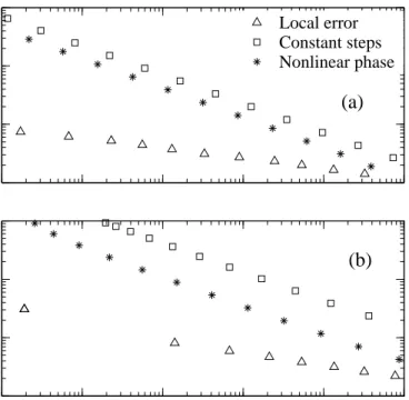
In Fig. 3.1, we have plotted the number of FFTs versus the global relative error for the dierent step-size criteria. Although the performance of the local error method is not signicantly better in the range of low accuracy values10−2₁₀−3_{, at high accuracy}

the computational cost of the local error method is one or two orders of magnitude less than for other methods. Notice that the nonlinear phase method performs better

(39)

103 104 105 106 Number of FFTs Local error Constant steps Nonlinear phase 10−7 10−6 10−5 10−4 10−3 10−2 104 105 106 107

Global relative error

Number of FFTs

(a)

(b)

Fig. 3.1: Plot of the total number of FFTs versus global relative errorεfor second-order (a) and fth-order (b) solitons.

than the constant step size method, consistent with the system's large nonlinearity. The slope of the local error method curve is less than those of the other two methods since the constant step size and nonlinear phase methods are globally second-order accurate, while the local error method is globally third-order accurate. The walk-o and constant step size methods are identical since this system includes only one type of ber. The logarithmic step size method reduces to the constant step size method because the ber is lossless, and (3.4) leads to a constant step size distribution.

Soliton Collisions

Soliton collisions can be a good test for numerical methods because the subtle eect of four-wave mixing cancellation after the collision is very sensitive to numerical errors [89]. The ber type and the initial pulse shape are the same as in the previous section, except thatA= 1. The pulse duration is 4 ps and the peak power is 8.8 mW.

(40)

10−7 10−6 10−5 10−4 10−3 10−2 10−1 102

103 104 105

Number of FFTs

Local error Constant steps Nonlinear phase

Fig. 3.2: Plot of the total number of FFTs versus global relative errorε_{for a collision of two}

rst-order solitons.

We launch two soliton pulses separated in time by 100 ps and with a central frequency dierence of 800 GHz. The number of Fourier modes is 3072 and the simulation time window is 400 ps. We show the performance of the dierent methods in Fig. 3.2. The

0

400

0 5000

Step size (m)

Distance (km)

Fig. 3.3: Step sizehas a function of distance for the local error method applied to a collision of two rst-order solitons.

local error, constant step size, and nonlinear phase rotation methods perform equally well at low accuracy, when the global error is in the range 10−3₁₀−1_{, while the local}

error method is much more ecient when the global error is less than 10−4_{. Global}

(41)

and to have them cancel out after the collision. The nonlinear phase method still works better than the constant step size method because the nonlinear interactions are critical in the propagation. As before, the logarithmic step size and walk-o methods reduce to the constant step size method.

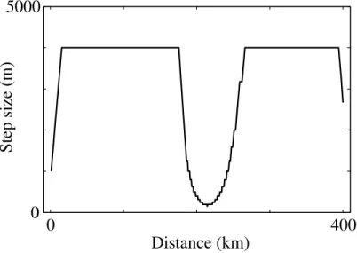
Using the example of a soliton collision, we illustrate the adaptive behavior of the local error algorithm. Fig. 3.3 shows the step size as a function of propagation distance for the soliton collision when the targeted range for the local error is (0.5×10−5_,₁₀−5₎

and the initial guess for the step size is 1000 m. Since the local error for this initial step is much less than the targeted range of values, at each step the step sizes are increased until the local error is within the targeted range. The pulse collision occurs at a distance of 200 km. At this point, we observe a signicant decrease in the step size, which is necessary to accurately resolve the collision. After the collision, the step size is increased to the same value as before the collision. The last step is smaller than the previous step simply because the remaining section of the ber is shorter than the step size chosen by the algorithm.

Single-Channel Systems

In this part we study periodically-stationary dispersion-managed soliton (DMS) and chirped-return-to-zero (CRZ) systems that resemble experimental systems [55], [94]. The DMS system is highly nonlinear, meaning that both dispersion and nonlinearity determine the signal evolution, while the CRZ system is quasi-linear and the evolution is mostly determined by dispersion [95]. Thus we are studying the four split-step implementations using two dierent types of systems. We include ber attenuation and gain, but we do not consider amplier noise. We use 64-bit random bit streams that repeat periodically. We stress that our goal is to test the performance of the numerical methods for realistic systems rather than to achieve optimal propagation. Consequently, it is important that we have pulse streams rather than single pulses,

(42)

that we use dispersion management, and that we include the eects of ber loss and amplier gain.

The DMS system is based on a 107 km dispersion map, which consists of four dispersion-shifted ber spans, each of 25 km, with normal dispersion equal to −1.10 ps/nm-km, followed by 7 km of standard single-mode ber with anomalous dispersion of 16.6 ps/nm-km at 1551 nm [94]. The loss in both bers is 0.21 dB/km, and the amplier spacing is 25 km with an additional amplier after the standard single-mode ber. We use Gaussian pulses with a FWHM duration of 9 ps, as is appropriate for a 10 Gbit/s bit rate. The peak power is 8 mW. The signal is launched in the middle of a span of anomalous ber to ensure the periodicity of the pulse shape as it propagates along the ber. The propagation distance is 1,280 km. The simu-lation time window is 6400 ps and the number of Fourier modes is 6144. We have not included a dispersion slope in this system since there is only a single channel and previous work indicates that higher-order dispersion plays no role [94].

The CRZ system is based on a 180 km dispersion map consisting of 160 km of dispersion-shifted ber with dispersion −2.44ps/nm-km, followed by 20 km of stan-dard ber with dispersion 16.55 ps/nm-km [55]. The dispersion slope is 0.075 ps2

/nm-km and the ber loss is 0.21 dB//nm-km for both bers, while the amplier spacing is 45 km. Symmetric dispersion pre- and post-compensation is performed using ber spans of length 2.0 km, where the dispersion is 93.5 ps/nm-km, the slope is −0.2ps2_{/nm-km and the loss is 0.5 dB/km. The initial pulses are phase-modulated,}

raised-cosine pulses with 1 mW peak power and a chirp parameter equal to−0.6[95]. The bit rate is 10 Gbit/s and the propagation distance is 1,800 km. The simulation time window is 6400 ps and the number of Fourier modes is 4096.

The performance of the four split-step implementations for the single-channel DMS and CRZ systems is shown in Figs. 3.4(a) and (b) respectively. In both systems, the local error method performs best over the entire range. Due to its higher order of

(43)

ac-10−6 10−5 10−4 10−3 10−2 10−1 102 103 104 105 Number of FFTs Local error Walk−off Nonlinear phase Log steps Constant steps 10−6 10−5 10−4 10−3 10−2 10−1 102 103 104 105 106

Number of FFTs

(a)

(b)

Fig. 3.4: Plot of the total number of FFTs versus global relative errorεfor the single-channel (a) DMS and (b) CRZ systems.

curacy, the data points for the local error method lie on a line with a smaller absolute slope than those of the other methods, as expected. However, all methods become comparable in the range of global errors10−3₁₀−1_{, the region of most interest in}

sim-ulating ber optic links. We note however, that in the CRZ system the performance of the logarithmic step size method is somewhat poorer than that of the nonlinear phase and walk-o methods.

Multi-Channel CRZ System

In order to compare the split-step implementations for modeling multi-channel com-munications systems, we used the same CRZ system as described above. In Fig. 3.5,

(44)

10−6 10−5 10−4 10−3 10−2 10−1 103

104 105 106

Number of FFTs Local error Walk−off Nonlinear phase Log steps Constant steps

Fig. 3.5: Plot of the total number of FFTs versus global relative errorε for the multichan-nanel CRZ system.

we show the performance of the split-step selection criteria on a 5-channel CRZ system with a 50 GHz channel spacing. As in the single-channel case, the local error method is much more ecient at high accuracy. However, at low accuracy, with the global error in the range10−3₁₀−1_{, the walk-o method performs best. At low accuracy, the}

local error method does not perform as well as the walk-o method for the following reasons. First, in the multi-channel CRZ system, the step size within each ber in the local error method varies approximately within a factor of two, and the average value is comparable to the step size in the walk-o method for a given global error. However, each pair of steps in the local error method is 50% more expensive than in the walk-o method. In addition, when the step size is large and the global accuracy is low, the higher-order solution u4 may not be as accurate as the ne solution uf.

Indeed, we have observed that the local error method performs slightly better at low global accuracy if we keep the ne solution uf instead of the higher-order solution u4

at each step.

Next, we observe that the nonlinear phase rotation method does not perform as well as the walk-o method in the multi-channel CRZ system, although the perfor-mance of the two methods is comparable in the single-channel DMS and CRZ systems.

(45)

There are two major reasons for this behavior. First, in contrast to the single-channel case, the walk-o criterion becomes more physically relevant in a WDM system, in which pulses in dierent channels collide. Second, the step size in the nonlinear phase rotation method is determined by the peak power in the time domain. In the single-channel CRZ system, the power function contains spikes due to the overlap between neighboring pulses. However, between ampliers the peak power decreases monotonically with distance due to ber attenuation. By contrast, the peak power of the multi-channel system does not decrease monotonically with distance but con-tains irregular spikes because pulses from dierent channels rapidly pass through each other. As a consequence, there is a signicant proportion of step sizes in the nonlinear phase rotation method that are much smaller than they need to be for a given global accuracy. The logarithmic step size method is not ecient in the CRZ system be-cause the step size choice is only based on limiting spurious four-wave mixing, which is only one of the potential sources of error in a multi-channel simulation. We also found that in the logarithmic step size method, the error grows most rapidly in bers with high dispersion. We nd that the constant step size method is inecient in the multi-channel CRZ system. The reason it performs so poorly is that for a given step size the global error does not accumulate linearly with distance. Consequently, in some sections of the transmission line the global error grows rapidly, while in others the error accumulates very slowly and computational eort is wasted.

In Figure 3.6, we show the step sizes in the local error method as a function of propagation distance when the targeted range for the local error is (0.5×10−4_, ₂_× 10−4_{). The upper two plots show the step sizes for the rst two and last two periods}

of the dispersion map, and the lower two plots show the corresponding portions of the dispersion map. The ampliers, marked by triangles, are placed after the pre-compensation ber, and then every 45 km. Notice that the step size increases as the signal power and the strength of the nonlinear interactions decrease due to the

(46)

0 300 0 500 1000 1500 Step size (m) 0 300 0 100 Distance (km) Dispersion (ps/nm/km) 1400 1800

Fig. 3.6: Step size h as a function of distance for the local-error method applied to the multichannel CRZ system. The upper two plots show the step sizes for the rst two and last two periods of the dispersion map, and the lower two plots show the corresponding portions of the dispersion map. Triangles indicate the positions of ampliers.

ber loss. Also note that step size is smaller in bers with higher dispersion since the pulses in neighboring channels move faster with respect to each other.

Variation of Method Parameters

In this part we address two important questions concerning how the method param-eter should be chosen to achieve a desired global accuracy. The method paramparam-eter is the parameter in a split-step method that we vary to adjust the accuracy of the method. First, for a given global error, how much does the method parameter depend on the particular system? Second, by what factor should the method parameter be decreased to halve the global error?