A harmonic balance method for nonlinear fluid structure interaction problems

A harmonic balance method for nonlinear fluid structure interaction

problems

W. Yao, S. Marques

⇑

School of Mechanical and Aerospace Engineering, Queen’s University Belfast, Belfast BT9 5AH, UK

a r t i c l e i n f o

Article history:

Received 2 September 2017 Accepted 12 February 2018

Keywords:

Limit cycle oscillations Vortex-induced vibrations Aeroelasticity CFD Harmonic balance Nonlinear

a b s t r a c t

Over the past decade the Harmonic-Balance technique has been established as a viable alternative to direct time integration methods to predict periodic aeroelastic instabilities. This article reports the pro-gress made in using a frequency updating procedure, based on a coupled fluid-structural solver using the Harmonic-Balance formulation. In particular, this paper presents an efficient implicit time-integrator that accelerates the convergence of the structural equations of motion to the final solution. To demonstrate the proposed approached, the paper includes a detailed investigation of the impact of input parameters and exercises the method for two types of fluid-structural nonlinear instabilities: transonic limit-cycle oscillations and vortex-induced vibrations.

Ó2018 The Authors. Published by Elsevier Ltd. This is an open access article under the CC BY license (http:// creativecommons.org/licenses/by/4.0/).

1. Introduction

The ever growing capability of computing hardware and soft-ware, enabled high fidelity computational fluid dynamics (CFD) to become the primary tool for the study of fluid physics. With sim-ilar advancements in computational structural dynamics (CSD) and coupling algorithms, CFD has also been extensively applied to fluid-structure interaction problems where flow nonlinearities such as shock waves or flow separation play a dominant role. The time dependency of this type of analysis means it usually requires additional computational resources. Nevertheless, fluid-structure interactions play a safety critical role in several applica-tions such as aircraft flutter or vortex induced vibration (VIV) fre-quency lock-in. Therefore, the efficient prediction of these and associated phenomena attracts much attention from the numerical methods research community.

Several alternatives to full time-domain simulations have been proposed to investigate the loss of linear stability of an aeroelastic system. Badcock et al. avoid conducting time-domain analysis by tracking the critical eigenvalue of the coupled system Jacobian matrix[1–3], at an equivalent cost of a few steady-state calcula-tions; if the Jacobian of the coupled system is not available, linear reduced-order models (ROM) can be built from prescribed time

domain simulations[4,5]and used to infer the system’s stability at a lower cost than using the full-order model.

If nonlinearities are present, additional instabilities have been observed which pose further challenges to the development of effi-cient simulation tools [6]. In particular, nonlinearities such as shocks, vortex shedding or free-play can cause periodic oscilla-tions, generally referred to as limit cycle oscillations (LCO) that are not captured by linear ROMs. Therefore, the development of nonlinear ROMs is a popular topic of research[7–10]. The system’s nonlinear response can be approximated based on input-output relations using a recursive nonlinear interpolator in lieu of the full order aerodynamic model[11–13]; Yao and Marques applied an input-output technique employing a radial basis function (RBF) neural network together with a discrete empirical interpolation method to reconstruct the complete flow field for the prediction of LCO[14].

The aforementioned nonlinear methods rely on performing time domain simulationsa priori, under specific conditions that enable a suitable nonlinear model for the problem to be built. Alternative methods have been proposed that preserve the under-lying physics of the problem and allow the direct computation of the nonlinear system. Following the stability analysis described in Refs.[1,3], LCO can be predicted by model order reduction using the critical eigenbasis of the Jacobian of the coupled system. Another alternative in this class of methods is to exploit the peri-odicity of the problem and solve the fluid-structural system in the frequency domain, these strategies are commonly known as Time-Spectral method or high-dimensional Harmonic Balance https://doi.org/10.1016/j.compstruc.2018.02.003

0045-7949/Ó2018 The Authors. Published by Elsevier Ltd.

This is an open access article under the CC BY license (http://creativecommons.org/licenses/by/4.0/). ⇑Corresponding author at: Department of Mechanical Sciences, University of

Surrey, Guildford GU2 7XH, UK.

E-mail addresses:[email protected],[email protected](S. Marques).

Contents lists available atScienceDirect

Computers and Structures

(HB) approach. The HB method transfers the time dependent prob-lem into a steady solution based on Fourier expansions. Originally applied in the context of CFD for turbomachinery problems[15,16], the HB method has been used in several diverse applications, including the prediction of dynamic derivatives[17,18], periodic flows found in rotorcraft[19]or wind-turbines[20]. Progress has also been made in applying the HB methodology to fluid structure interaction. For the majority of such cases, it is worth noting that the fundamental frequency of the oscillation is not knowna priori and is an additional unknown. Thomas et al. developed the HB/LCO method to predict LCO based on a Newton–Raphson approach, where a HB formulation solves the fluid problem and amplitude and frequency are determined simultaneously[21]. Blanc et al. proposed a fully coupled aero-structural Harmonic Balance solver for forced motions. Ekici and Hall also developed a fully coupled fluid-structure coupled HB strategy capable of predicting LCOs for one degree-of-freedom (DOF) turbomachinery components [22]. Yao and Marques, building upon these approaches, proposed an Aeroelastic-HB (A-HB) to analyze fixed wing nonlinear aeroelas-tics[23]and this was further adapted to VIV lock-in by Yao and Jai-man[24].

The A-HB approach and its version developed for VIV employs an explicit scheme to resolve the structural equations of motion, together with a relaxation approach to update the fundamental frequency of the oscillation. Both these strategies limit the efficiency of the iterative scheme. This paper addresses these limitations by reformulating the A-HB method using an approximate exponential time differencing scheme and subsequent modified strategy to update the frequency. The following sections will describe the numerical formulation for the flow and structural models, this is followed by the introduction of the new coupling procedure; the final two sec-tions of the paper present a diverse range of test cases used to critique the new A-HB method and the conclusions obtained from this work.

2. Aeroelastic - harmonic balance formulation 2.1. Fluid governing equation

The governing fluid equations used in this work are the com-pressible Euler or laminar Navier-Stokes equations. For time-dependent problems with moving boundaries, the system of equa-tions is solved using an arbitrary Lagrangian-Eulerian (ALE) formu-lation as follows:

dw

dt ¼ RðwÞ ð1Þ

RðwÞ ¼

r

Fi_Fv_{; ð2Þ}

the integral form of these equations for a control volumeVj with surfacedScan be written as:

d dt Z VjðtÞ w dV þ I @VjðtÞ Qn dS¼0 ð3Þ and Q¼ ðFiFvwvgÞ; ð4Þ

wheretis the physical time,w¼½

q

;

q

u;

q

ET

is the vector of con-served variables, the over-bar denotes the control volume average quantities;

_q

is the density andEis the energy,uand

v

g are the Cartesian flow and grid velocities vectors, respectively and n is the outward unit normal of every cell face.Fi andFv correspond to the inviscid and viscous fluxes, respectively and can be written in compact form as:

Fi¼

q

u

q

uiuþpdij ð

q

EþpÞup

v

g 2 64 3 75; Fv¼ 0

s

ij

s

ijuqi 2 64 3 75; i¼1;2;3: ð5Þ

The inviscid flux is calculated by the AUSMþup flux function [25], together with the Van Albada limiter to achieve 2nd order spatial accuracy, details of this implementation can be found in Ref. [26]. The viscous stress tensor

_s

ij and the heat flux qi are given by:

s

ij¼

l

@ ui @xjþ @uj @xi 2 3 @uk @xkd ij ð6Þ qi¼

l

cp Pr @T @xi ð 7Þ

where

_l

is the coefficient for laminar viscosity,cpis the specific heat ratio for a perfect gas andPr¼0:72 is the laminar Prandtl number. The pressure is given by the ideal gas law:

p¼ ð

c

1Þ

q

E1

2ðuuÞ

ð8Þ

where

c

¼1:4 and represents the ratio of specific heats for a dia-tomic gas.

Following Hall et al. [16], Eq. (1) can be written in the high dimensional HB format as

x

DwhbþRhb¼0; ð9Þ

where

x

is the system’s fundamental frequency,whb andRhbare the fluid and residual solution at equally spaced time intervals Dt¼T=ð2NHþ1Þ where T¼2

p

=

x

and NH corresponds to the number of harmonics selected. The matrixDis given by: Di;k¼ 2 2NHþ1 XNH n¼1 nsin 2

p

nðkiÞ 2NHþ1 : ð10Þ

Full details of the HB implementation and derivation of matrixD

can be found in Refs.[23,27]. The Eq.(9)is solved by introducing a pseudo time variable,

s

:

dwhb

d

_s

þ

x

DwhbþRhb¼0: ð11Þ

This means that the time dependency of the fluid equation is converted into a steady problem. An LU-SGS [28] scheme is employed to March the Eq.(11)forward in pseudo-time.

2.2. Structural governing equations

The equations of motion for a linear structural model can be described in general terms as

M

g

€þf

g

_þK

g

¼f; ð12Þ

hereM; f; Kare the mass, damping and stiffness matrices of the structure,

g

andf are the displacement and external force applied to the structure. The latter two quantities also correspond to the output and input to the structural system. The structural equations in state space format can be described as,

_ n¼AsnþBsf ð13Þ where As¼ 0 I M1_{K M}1 f ; Bs¼ 0 M1 ; n¼

g

_g

_{_} :

Similar to the fluid equations, the same HB operatorDcan be applied to Eq.(13), resulting in

The structural residualL2norm is then defined L2¼1 2R T sRs ð15Þ and Rs¼ ð

x

DAsÞ

g

hbBsfhb ð16Þ

2.3. Harmonic-balance fluid structure coupling

The basic idea in the original A-HB method proposed by Yao and Marques[23], is to transform the fluid structure interaction prob-lem in the frequency domain with a fixed point algorithm, which is repeated inAlgorithm 1.

Algorithm 1. A-HB

In the original A-HB approach, a direct solver with a relaxation factor, Eq.(17), was adopted for step 2 inAlgorithm 1, which can be considered as a one step explicit algorithm. However, the relax-ation factorkrestricts the convergence rate.

g

n hb¼

g

n1

hb þkð

g

^hb

g

hbn1Þ; ð17Þ

where

g

^hb¼ ðxDAsÞ1Bsfnhb. An alternative time integrator for the structural system is necessary to lift up this restriction. Following Ekici and Hall[22]and similar to Eq.(11), a pseudo time stepping is introduced in Eq.(14) to integrate in time the HB form of the structural equations:

_

g

hb¼Asd

g

hbþBsfhb ð18Þ

whereAsd¼ ðxDAsÞ.

The exact discretization of Eq.(18)is given by[29]

g

n hb¼eAsdDs

g

nhb1þ Z nDs ðn1ÞDse AsdðnDsrÞ_B sfhbð

r

Þd

r

: ð19Þ

The integral term in Eq. (19) can be simplified by defining

t

¼nDs

r

, andfhbðrÞ ¼1=2ðfnhbþfnhb1Þ, resulting in

g

n hb¼e AsdDs

g

n1 hb þ 1 2A 1 sdðe AsdDs_IÞ_B sðfnhbþfn 1 hb Þ: ð20Þ

The practicality of this result depends on the evaluation of the matrix exponential. To improve robustness, the matrix exponential is approximated aseAsdDsð_IDs_AsdÞ1_{, this corresponds to a first}

order Padé type approximation[30]. Additionally Eq.(20)can be simplified by noting that

Asd1 e AsdDs_I Asd1 ðI

D

s

AsdÞ1I h i ¼Asd1½IðI

D

s

AsdÞðI

D

s

AsdÞ 1 ¼

D

s

ðI

D

s

AsdÞ 1 ; ð21Þ

which leads to:

g

n hb¼ ðIAsdD

s

Þ 1

_g

n1 hb þ 1 2

D

s

Bsðf n hbþf n1 hb Þ : ð22Þ

This exponential time integrator is the same as a first order linearly implicit one, in which the force termfhbis approximated by the Trapezoidal rule. A standard implicit Euler method can be recovered by assuming constantfhborfðrÞ ¼fnhbin the exact discretization Eq.

(19). The results shown in the next section suggest that the conver-gence rate of Eq.(22)improves significantly with respect to the standard implicit method. Therefore, the Eq.(17)in step 2 of

Algo-rithm 1is replaced by Eq.(22).

Unlike the time accurate fluid and structure interaction compu-tation,Algorithm 1is typically a steady state searching process, where only the converged solution matters. The frequency

x

is updated by minimizing the system’s residual L2 norm [31,22],

defined in Eq.(15), by using the gradient with respect to the fre-quency, which in this work is given by:

@L2 @

x

¼ D

g

hbBs@fhb @

x

T ð

x

DAsÞ

g

Bsfhb ½ ð23Þ

Previously, the authors demonstrate that@fhb

@x, which is computed by finite differencing, improves the frequency updating process signif-icantly, however this is dependent on the step size used. By intro-ducing the implicit method in step 2 in the A-HB method the impact of the force derivative becomes less significant to the overall efficiency of the algorithm (results indicate up to 10% reduction in computing time).

The modified A-HB method is referred to A-HB+ method. The controlling parameters for the A-HB+ method are defined as ½Ds;NH;Ni;

x

0;

g

0, where Ds;NH;Ni;

x

0;

g

0 are the pseudo time

step, number of harmonics, number of sub-iterations, initial fre-quency and displacement, respectively.

In the next section, the sensitivity of the A-HB+ method with respect to these parameters is investigated using a pitch/plunge transonic aerofoil system, undergoing an LCO; following this initial problem, the proposed method is tested to predict LCOs for the Goland wing and the versatility of the approach is further demon-strated by predicting oscillations due to vortex shedding.

3. Results

3.1. Aerofoil aeroelastic system

To assess the A-HB+ method, a NACA 64A010 aerofoil with pitch (

_a

) and plunge (h) DOF is adopted. The non-dimensional structural governing equation, Eq. (24), and parameters given in Table 1 follow the descriptions found in Refs.[21,23]:

M

g

€þ1 V2K

g

¼ 4

p.

f ð24Þ where M¼ 1 xa xa r2a ; K¼ xxha 2 0 0 r2 a 2 4 3 5_{; f ¼} Cl 2Cm ;

g

¼ 2ch

a

" # ; V¼U1

x

ac: Table 1

Pitch/plunge aerofoil parameters.

Static unbalance,x_a 0.25

Radius of gyration about elastic axis,r2 a 0.75

Frequency ratio,xh=xa 0.5

Mass ratio,.¼4m=pq1c2

U1represents the freestream velocity,Clis the lift coefficient and

Cm is the pitching moment coefficient. Critical conditions are set using the velocity index is defined asVs¼2U1=ðxacp Þffiffiffi

.

, and then

applying the procedure given byAlgorithm 1.

The fluid domain is descritized using an O-type grid with 12141 points in the circumferential and radial direction, respec-tively; the solution of the fluid problem is obtained by solving the Euler equations. The Mach number and initial angle of attack are, respectively,½M1;

a

0 ¼ ½0:8;0. The CFL number is set to 1 and

kept the same for all the LCO calculations.

First, the number of harmonics required to converge this problem with the time integrator from Eq. (22) is investi-gated. Conditions are set as: ½Ds;Ni;

j

0 ¼ ½50;100;0:105,

g

0¼ ½0:2;0:02

T_,V

s¼0:8. The A-HB+ method starts with the ini-tial flow solution computed with ½j0;

g

0, where

j

¼U21xc is the reduced frequency and

_j

0 is near to the flutter onset frequency

(

_j

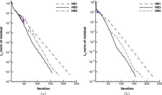
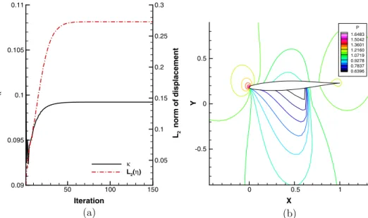
flutter0:109)[23].Fig. 1shows the fluid and structure conver-gence history, which indicates both fluid and structural residual

converge rapidly. The stopping criteria is based on the structural residual reducing 15 orders of magnitude. As shown in Fig. 2, both plunging and pitching amplitudes converge when using three harmonics (NH¼3), the fully reconstructed cycle using three harmonics (cycle HB3), shows good agreement with the conventional time-domain (TD) result. Fig. 3(a) shows that the LCO solution (½j;

g

) converges after approximately 100 iterations with the corresponding structural residual near 1010. The shock motion drives the aerodynamic forces and Fig. 3(b) shows the aerofoil motion at the maximum plunging position, while pitch-ing nose down.

After theNHconvergence study, the time integrator from Eq.

(22)is compared against the standard implicit temporal discretiza-tion with½Ds;NH;Ni;

j

0 ¼ ½50;3;100;0:105,

g

0¼ ½0:2;0:02

T

.Fig. 4

shows that Eq.(22) improves the convergence rate significantly with respect to the standard first order implicit method. Therefore, the solution of Eq.(22)is the default setting in A-HB+ method and adopted for the remainder of the calculations.

Iteration L2 nor m of r e s idua l 50 100 150 200 250 10-8 10-7 10-6 10-5 10-4 10-3 10-2 10-1 100 HB1 HB3 HB5 Iteration L2 nor m of r e s idua l 50 100 150 200 250 10-16 10-14 10-12 10-10 10-8 10-6 10-4 10-2 100 HB1 HB3 HB5

Fig. 1.L2norm of residual of (a) fluid and (b) structure with different number of harmonics.

h h -0.4 -0.2 0 0.2 0.4 -0.1 -0.05 0 0.05 0.1 0.15 TD cycle_HB3 HB1 HB3 HB5 α . _α -0.04 -0.02 0 0.02 0.04 -0.01 0 0.01 0.02 TD cycle_HB3 HB1 HB3 HB5

Fig. 2.LCO position-velocity diagram retaining different number of harmonics: (a) plunging and (b) pitching. The large symbols correspond to the time intervals solved by the A-HB+ method.

The sensitivity of the time step size Ds is performed by using _½NH;Ni;

j

0 ¼ ½3;100;0:105,

g

0¼ ½0:2;0:02

T_{, and}

Ds¼ ½10;25;50;100;1000. Fig. 5 suggests that values between

106Ds6100 produce adequate convergence rates, with the opti-mum being nearDs¼50. The results indicate that the time step size if enlarged arbitrarily, deteriorates the convergence rate, but the system remained stable up toDs¼1000; it is worth noting that the standard implicit formulation convergence stalled for DsP100 at a value of 108_.

The initial guess for the frequency

_j

0is normally chosen near

the flutter onset frequency. The flutter onset can be predicted by several approaches as described in the introduction. Nevertheless, the sensitivity to this parameter is carried out by using ½Ds;NH;Ni ¼ ½50;3;100,

g

0¼ ½0:2;0:02

T _and

j

¼ ½0:08;0:15.

Fig. 6 shows the initial frequency and updating strategy impact

on the convergence rate. The inclusion of the force derivative in Eq.(23)has a stronger influence on the convergence for poorer ini-tial frequency estimates. However, and unlike the original A-HB

method, this typically yields less than 10% computational savings, both in the number of iterations and in time. Overall, the LCO solu-tion converges within 160–220 iterasolu-tions, even for the case where the initial frequency deviated approximately 50% from final solu-tion. The solution to this problem using the original A-HB method took nearly 1 h, the current method reduces the computational elapsed time by approximately a factor of two.

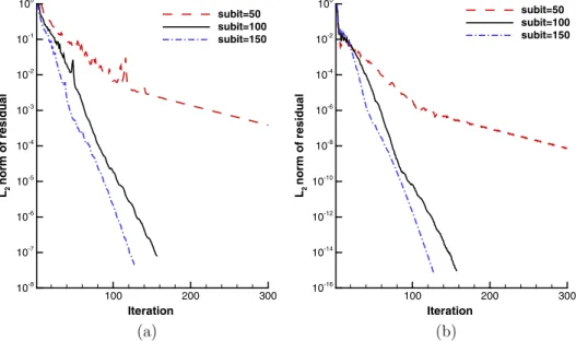
The A-HB+ coupling process is a steady state computation, therefore, it is not necessary to drive the fluid residual to a very low level for each sub-iteration, unlike time domain loosely cou-pled, aero-structural solvers. However, the number of iterations (Ni) has a significant impact on the convergence rate as shown in

Fig. 7; the inputs used are ½Ds;NH;

j

0 ¼ ½50;3;0:105 and

g

0¼ ½0:2;0:02

T_{. There is a marginal speed up in convergence when} increasingNifrom 100 to 150, whereas there is a deterioration for

Iteration κ L2 n o rm o f d is p lacemen t 50 100 150 0.09 0.095 0.1 0.105 0.11 0.05 0.1 0.15 0.2 0.25 0.3 κ L2(η) X Y 0 0.5 1 -0.5 0 0.5 P 1.6483 1.5042 1.3601 1.2160 1.0719 0.9278 0.7837 0.6396

Fig. 3.(a) DisplacementL2norm and reduced frequency convergence history and (b) pressure contour nearhmax.

Fig. 4.L2 norm of the structural residual using the proposed approximate

exponential integrator, Eq.(22), and the standard implicit Euler method.

Iteration L2 nor m of r e s idua l 100 101 102 103 10-14 10-12 10-10 10-8 10-6 10-4 10-2 100 Δτ=10 Δτ=25 Δτ=50 Δτ=100 Δτ=1000

Ni¼50. Therefore, Ni¼100 is considered sufficient for the 2D aerofoil case.

The parameter sensitivity study shows that the method is robust and accurate and provides a guideline to chose adequate parameter combinations.

3.2. Goland wing aeroelastic system

The second test case is the Goland+ _{wing structure (the +}

denotes the heavy version of the wing) with a tip store. The pur-pose of this problem is to investigate and exercise the A-HB+ method for 3D fixed-wing LCO problems. This case has been reported in the literature to exhibit aeroelastic instabilities, both flutter and LCOs, driven by the presence and oscillation of shock-waves [32–34,1,35,36]. Results reported in the cited literature, show the presence of a transonic flutterbucket near M1¼0:92

where both modes 1 and 3 are lightly damped, driven by the pres-ence of a shock-wave near the trailing edge of the wing, which can result in a LCO.

The wing is of rectangular shape, with a semi-span and chord length (c) of 6.096 m, 1.8288 m, respectively, and the thickness-to-chord-ratio (

s

) is 0.04. The aerofoil profile consists of a parabolic arc, constant along the span, given by:

z c¼ 2

s

1 x c _x c ð25Þ

A linear finite element model (FEM), shown here inFig. 8(a), was built following the details provided by Beran et al. [33], but the presence of the tip store is not reflected in the CFD mesh, as illus-trated inFig. 8(b). The CFD mesh follows anO-topology and has a total of 69,741 cells, with 81 points along the semi-span and 41 along the chord direction. The structural mode shapes and natural

Iteration Wall clock [s] L2 norm of residual 50 100 150 200 0 500 1000 1500 10-16 10-14 10-12 10-10 10-8 10-6 10-4 10-2 100 κ=0.08 κ=0.15 Iteration Wall clock [s] κ 50 100 150 200 0 500 1000 1500 0.08 0.1 0.12 0.14 0.16 κ=0.08 κ=0.15

Fig. 6.(a)L2norm of structural residual and (b) reduced frequency convergence with different initial frequencies (the symbols denote results that include the force derivative

in the frequency updating procedure).

Iteration L2 nor m of r e s idua l 100 200 300 10-8 10-7 10-6 10-5 10-4 10-3 10-2 10-1 100 subit=50 subit=100 subit=150 Iteration L2 nor m of r e s idua l 100 200 300 10-16 10-14 10-12 10-10 10-8 10-6 10-4 10-2 100 subit=50 subit=100 subit=150

frequencies are obtained by using the software MSC/NASTRAN. The first four normal modes, depicted inFig. 9, are retained for the LCO analysis.

The problem is initially set up with the knowledge of the flutter conditions from the reported literature. The input parameters for the A-HB+ method are½M1;

a ¼ ½

0:92;0;½Ds;NH;Ni ¼ ½25;3;50,

g

0¼ ½2;1;0:1;0:1

T

and

_j

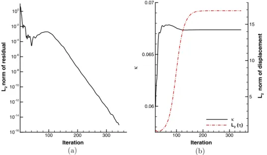
¼0:06; in addition, all results employ standard sea-level air density. A reference LCO is sought at U1¼137:16 m s1 which is about 15% above the flutter onset

condition reported by Snyder et al.[32]. For these conditions, the structural residual reaches 1010 after approximately 200

iterations as shown inFig. 10(a). The LCO frequency and amplitude converge as depicted inFig. 10(b).

Next, further LCO conditions were computed for freestream velocities below and above 137:16 m s1_{, which show the}

develop-ment of a supercritical LCO branch,Fig. 11(a), with the amplitude increasing rapidly beyondU1¼116 m s1. The flutter and LCO

conditions result from the interaction between mode 1 (first bend-ing) and mode 2 (first torsion). Results are consistent with those reported by Beran et al. [33] using conventional time-domain methods. There is a small change in the frequency between 116 m s1 _{and 125 m s}1_{, beyond this point the frequency}

X Z Y X Z Y Fig. 8.Goland+

(a) FEM model and (b) CFD mesh.

Fig. 9.Structural normal modes projected onto the CFD grid: (a) Mode 1 (1.71 Hz), (b) Mode 2 (3.05 Hz), (c) Mode 3 (9.20 Hz), and (d) Mode 4 (10.90 Hz).

Iteration L2 norm of residual 100 200 300 10-16 10-14 10-12 10-10 10-8 10-6 10-4 10-2 100 Iteration κ L2 norm of displacement 100 200 300 0.06 0.065 0.07 5 10 15 κ L2 (η)

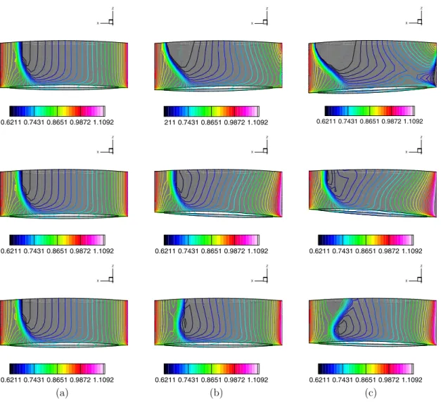
increases at an accelerating rate. The corresponding shock motion atU1¼ ½116;120;125m s1is represented by the pressure field

at three time-slices from the HB calculation in Fig. 12. At U1¼116 m s1, the shock exhibits small fluctuations, but its

position remains largely unchanged. AtU1¼120 m s1, the wing

twist at the tip increases, the shock excursion at the wing root is

significant and during the cycle, a strong region of lower pressure extends towards the wing tip; overall significant changes in sur-face pressure occur both at the wing’s tip and root. At speeds of U1¼125 m s1, the shock at the root reaches the trailing edge

and it weakens as it moves forward, atU1¼137:16 m s1all but

vanishes. For speeds aboveU1¼125 m s1, the frequency starts U [ms-1 ] Generalized Coordinate 110 115 120 125 130 135 140 0 0.5 1 1.5 2 2.5 3 _{Mode 1} Mode 2 U [ms-1] Frequency [Hz] 110 115 120 125 130 135 140 2.5 2.55 2.6 2.65 2.7 2.75 2.8

Fig. 11.LCO development with velocity: (a) amplitude and (b) frequency.

X Y Z 0.6211 0.7431 0.8651 0.9872 1.1092 X Y Z 211 0.7431 0.8651 0.9872 1.1092 X Y Z 0.6211 0.7431 0.8651 0.9872 1.1092 X Y Z 0.6211 0.7431 0.8651 0.9872 1.1092 X Y Z 0.6211 0.7431 0.8651 0.9872 1.1092 X Y Z 0.6211 0.7431 0.8651 0.9872 1.1092 X Y Z 0.6211 0.7431 0.8651 0.9872 1.1092 X Y Z 0.6211 0.7431 0.8651 0.9872 1.1092 X Y Z 0.6211 0.7431 0.8651 0.9872 1.1092

to increase and the low pressure region observed at the wing tip leading edge, extends further inboard, originating large pressure differentials, sustaining higher amplitudes.

3.3. Circular cylinder VIV system

This case presents a different type of self sustained oscillations, i.e. driven by vortex shedding. For elastic immersed structures, the vortex shedding frequency can depart from the Strouhal frequency and become synchronized, orlocked in, with the frequency of the structure’s motion; this nonlinear coupling between the vortex shedding and structure results in self limiting oscillations. Recently, Yao and Jaiman demonstrated how the lock-in frequency and motion amplitude can be determined using the A-HB approach

inAlgorithm 1. In this section, the A-HB+ formulation is evaluated

for VIV problems.

Consider the nondimensional structural equation for a vibrating cylinder with 2-DOF:

M€

g

þf

g

_þK

g

¼f ð26Þ where M¼ 1 0 0 1 ; f¼ 4

1p

Fs 0 0 4

1p

Fs ; K¼ ð2

p

FsÞ 2 0 0 ð2

p

FsÞ 2 " # f¼ 2

p

m Cl Cd ;

g

¼ x y ;

here thexandyare the horizontal and vertical displacements;Cl andCd are the lift and drag coefficient,m;

1

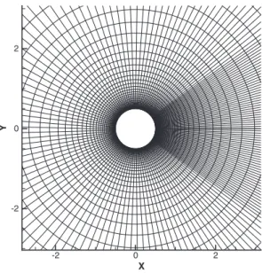
are the mass ratio and damping coefficient, respectively. Following convention, the reduced natural frequency is defined asFs¼1=Ur, whereUr is the reduced velocity. The mass ratiom is defined as the ratio between the vibrating structure and the mass of displaced fluid.

The fluid domain is discretized with 17165 points in the cir-cumferential and radial directions respectively, with the outer boundary located 50 diameter lengths away from the cylinder’s centre; the resultant mesh and point distribution near the surface X Y -2 0 2 -2 0 2

Fig. 13.Mesh around cylinder for VIV problem.

Iteration L2 n o rm o f resi d u al 500 1000 1500 2000 10-16 10-14 10-12 10-10 10-8 10-6 10-4 10-2 100 Iteration κ L2 nor m of dis p la c e m e nt 500 1000 1500 2000 0.4 0.45 0.5 0.55 0.5 1 1.5 2 2.5 κ L2 (η)

Fig. 14.The convergence of (a) structural residual and (b) VIV response.

X Y 0.09 0.1 0.11 0.12 0.13 -0.6 -0.4 -0.2 0 0.2 0.4 0.6 TD Cycle_HB5 HB5

is illustrated in Fig. 13. The fluid problem is solved assuming laminar flow.

The inputs to the A-HB+ solver are: _½m_;Ur;

1 ¼ ½

10;6;0:0, ½M1;Re ¼ ½0:3;100, whereRecorresponds to the Reynolds

num-ber, ½Ds;NH;Ni ¼ ½25;5;50 and with the initial displacement of

g

0¼ ½0:1;0:5

T_{. The initial frequencyf}

0¼1=Uris used for the VIV computation. Hence, for a given Reynolds number and remainder input conditions, the A-HB+ solver determines the corresponding locked-infrequency and amplitude, if they exist. Based on the find-ings by Yao and Jaiman[26], for 2-DOF vortex shedding problems, five harmonics are retained to fully capture the nonlinear motion and flow characteristics. This results in several more iterations than what was observed in the previous two cases, as shown in

Fig. 14. The trajectory obtained for the cylinder is shown in

Fig. 15; agreement with the time domain result is excellent.

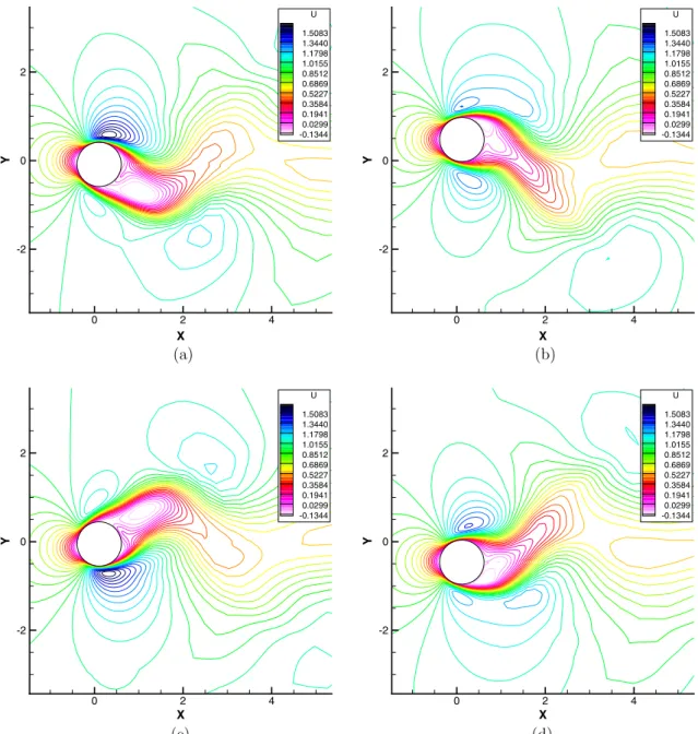
Illus-tration of the velocity field at four distinct points is shown in

Fig. 16, detailing the cylinder’s extreme heave positions and

speeds. The alternating vortex shedding on opposite sides of the motion cycle is clearly captured.

4. Conclusions

A new HB methodology to predict periodic, nonlinear fluid-structures interaction problems, was proposed and demonstrated. By implementing a particular implicit structural time integrator, that largely removes the restrictions on the scheme’s time step, the convergence of the HB equations of motion to the final amplitude-frequency combination is accelerated. The necessity to approximate force derivatives to converge on the final frequency remains advantageous but is now secondary.

The proposed method was demonstrated for three test cases. The first case analyzed was a 2-DOF aerofoil undergoing an LCO that was the focus of the original A-HB method study; a detailed parametric investigation of the new approach showed an improved robustness and consistent results over a wide range of conditions. The Goland+_{wing allowed exercising the method for a fixed wing}

undergoing LCO at a transonic Mach number and over a range of different dynamic pressures. The last test case featured a fluid-structure instability driven by vortex-shedding exciting a self

X Y 0 2 4 -2 0 2 U 1.5083 1.3440 1.1798 1.0155 0.8512 0.6869 0.5227 0.3584 0.1941 0.0299 -0.1344 X Y 0 2 4 -2 0 2 U 1.5083 1.3440 1.1798 1.0155 0.8512 0.6869 0.5227 0.3584 0.1941 0.0299 -0.1344 X Y 0 2 4 -2 0 2 U 1.5083 1.3440 1.1798 1.0155 0.8512 0.6869 0.5227 0.3584 0.1941 0.0299 -0.1344 X Y 0 2 4 -2 0 2 U 1.5083 1.3440 1.1798 1.0155 0.8512 0.6869 0.5227 0.3584 0.1941 0.0299 -0.1344

sustained oscillation. The ability of the A-HB+ to determine the so called locked-in conditions is demonstrated for a 2-DOF vibrating cylinder. For all test cases, the A-HB+ provided detailed informa-tion on the periodic oscillatory flow characteristics and structural motion. Results indicate the computational effort was reduced by a factor of two with respect to the original A-HB method.

Acknowledgements

This work was sponsored by the United Kingdom Engineering and Physical Sciences Research Council (Grant No. EP/ P025692/1). The authors gratefully acknowledged this support.

References

[1]Woodgate MA, Badcock KJ. Fast prediction of transonic aeroelastic stability and limit cycles. AIAA J 2007;45(6):1370.

[2]Badcock K, Woodgate M. Bifurcation prediction of large-order aeroelastic models. AIAA J 2010;48(6):1037–46.

[3] Badcock K, Timme S, Marques S, Khodaparast H, Prandina M, Mottershead J, et al. Transonic aeroelastic simulation for instability searches and uncertainty analysis. Prog Aerosp Sci 2011;47(5):392–423. https://doi.org/10.1016/ j.paerosci.2011.05.002.

[4]Lucia DJ, Beran PS, Silva WA. Reduced-order modeling: new approaches for computational physics. Prog Aerosp Sci 2004;40(1):51–117.

[5]Silva W. Identification of nonlinear aeroelastic systems based on the Volterra theory: progress and opportunities. Nonlin Dynam 2005;39(1–2):25–62. [6] Dowell EH. Some recent advances in nonlinear aeroelasticity: fluid-structure

interaction in the 21st century. In: 51st AIAA/ASME/ASCE/AHS/ASC structures, structural dynamics, and materials conference; 2010.

[7]Chaturantabut S, Sorensen DC. Nonlinear model reduction via discrete empirical interpolation. SIAM J Scient Comput 2010;32(5):2737–64. [8]Carlberg K, Farhat C, Cortial J, Amsallem D. The {GNAT} method for nonlinear

model reduction: effective implementation and application to computational fluid dynamics and turbulent flows. J Comput Phys 2013;242:623–47. [9] Brunton SL, Proctor JL, Kutz JN. Discovering governing equations from data by

sparse identification of nonlinear dynamical systems. Proc Nat Acad Sci 2016;113(15):3932–7.https://doi.org/10.1073/pnas.1517384113.

[10]Yao W, Liou M-S. A nonlinear modeling approach using weighted piecewise series and its applications to predict unsteady flows. J Comput Phys 2016;318:58–84.

[11] Mannarino A, Mantegazza P. Nonlinear aeroelastic reduced order modeling by recurrent neural networks. J Fluids Struct 2014;48:103–21.https://doi.org/ 10.1016/j.jfluidstructs.2014.02.016.

[12] Lindhorst K, Haupt M, Horst P. Efficient surrogate modelling of nonlinear aerodynamics in aerostructural coupling schemes. AIAA J 2014;52 (9):1952–66.https://doi.org/10.2514/1.J052725.

[13] Yao W, Liou M-S. Reduced-order modeling for flutter/lco using recurrent artificial neural network. In: 12th AIAA aviation technology, integration, and operations (ATIO) conference and 14th AIAA/ISSM; 2012.

[14]Yao W, Marques S. Nonlinear aerodynamic and aeroelastic model reduction using a discrete empirical interpolation method. AIAA J 2017;55(2):624–37. [15]Ning W, He L. Computation of unsteady flows around oscillating blades using

linear and nonlinear harmonic euler methods. Trans-Am Soc Mech Engin J Turbomach 1998;120:508–14.

[16] Hall KC, Thomas JP, Clark WS. Computation of unsteady nonlinear flows in cascades using a harmonic balance technique. AIAA J 2002;40(5):879–86. https://doi.org/10.2514/2.1754.

[17] Hassan D, Sicot F. A time-domain harmonic balance method for dynamic derivatives predictions. In: 49th AIAA aerospace sciences meeting including the new horizons and aerospace exposition; 2011. p. 4–7.

[18]Da Ronch A, McCracken AJ, Badcock KJ, Widhalm M, Campobasso M. Linear frequency domain and harmonic balance predictions of dynamic derivatives. J Aircr 2013;50(3):694–707.

[19]Woodgate M, Barakos G. Implicit computational fluid dynamics methods for fast analysis of rotor flows. AIAA J 2012;50(6):1217–44.

[20]Campobasso MS, Baba-Ahmadi MH. Analysis of unsteady flows past horizontal axis wind turbine airfoils based on harmonic balance compressible Navier-Stokes equations with low-speed preconditioning. J Turbomach 2012;134 (6):061020.

[21]Thomas JP, Dowell EH, Hall KC. Nonlinear inviscid aerodynamic effects on transonic divergence, flutter, and limit-cycle oscillations. AIAA J 2002;40 (4):638–46.

[22]Ekici K, Hall KC. Harmonic balance analysis of limit cycle oscillations in turbomachinery. AIAA J 2011;49(7):1478–87.

[23]Yao W, Marques S. Prediction of transonic limit-cycle oscillations using an aeroelastic harmonic balance method. AIAA J 2015;53(7):2040–51. [24] Yao W, Jaiman RK. A harmonic balance technique for the reduced-order

computation of vortex-induced vibration. J Fluids Struct 2016;65:313–32. https://doi.org/10.1016/j.jfluidstructs.2016.06.002.

[25]Liou M-S. A sequel to ausm, part ii: Ausm+-up for all speeds. J Comput Phys 2006;214(1):137–70.

[26] Yao W, Marques S. Application of a high-order CFD harmonic balance method to nonlinear aeroelasticity. J Fluids Struct, doi: https://doi.org/10.1016/j. jfluidstructs.2017.06.014[in press].

[27]Hayes R, Marques SP. Prediction of limit cycle oscillations under uncertainty using a harmonic balance method. Comp Struct 2015;148:1–13.

[28] Yoon S, Jameson A. Lower-upper symmetric-Gauss-Seidel method for the Euler and Navier-Stokes equations. AIAA J 1988;26(9):1025–6. https://doi.org/ 10.2514/3.10007.

[29] Williams RL, Lawrence DA. State-space fundamentals. John Wiley & Sons, Inc.; 2007. p. 48–107.https://doi.org/10.1002/9780470117873.ch2.

[30]Kleefeld B, Khaliq A, Wade B. An ETD Crank-Nicolson method for reaction-diffusion systems. Numer Meth Partial Diff Eq 2012;28(4):1309–35. [31]McMullen M, Jameson A, Alonso J. Demonstration of nonlinear frequency

domain methods. AIAA J 2006;44(7):1428–35.

[32] Snyder R, Scott J, Khot N, Beran P, Zweber J. Predictions of store-induced limit-cycle oscillations using Euler and Navier-Stokes fluid dynamics. In: 44th AIAA/ ASME/ASCE/AHS/ASC structures, structural dynamics, and materials conference; 2003, doi:https://doi.org/10.2514/6.2003-1727.

[33] Beran PS, Khot NS, Eastep FE, Snyder RD, Zweber JV. Numerical analysis of store-induced limit-cycle oscillation. J Aircr 2004;41(6):1315–26.https://doi. org/10.2514/1.404.

[34]Beran PS, Strganac TW, Kim K, Nichkawde C. Studies of store-induced limit-cycle oscillations using a model with full system nonlinearities. Nonlin Dynam 2004;37(4):323–39.

[35] Marques S, Badcock K, Khodaparast H, Mottershead J. Transonic aeroelastic stability predictions under the influence of structural variability. J Aircr 2010;47(4):1229–39.https://doi.org/10.2514/1.46971.

[36] Marques S, Badcock K, Khodaparast H, Mottershead J. How structural model variability influences transonic aeroelastic stability. J Aircr 2012;49 (5):1189–99.https://doi.org/10.2514/1.C031103.