Discussion Papers No. 576, January 2009
Statistics Norway, Research Department
Christian N. Brinch
The effect of benefits on disability
uptake
Abstract:
I study the effects of the level of disability benefits on disability uptake. Estimation of such effects is difficult because individual levels of disability pension benefits are closely related to individual characteristics that may also affect disability uptake through other mechanisms. I exploit variation in disability benefits related to individual characteristics only through birth cohort, due to special rules of the phasing in of the Norwegian National insurance scheme. These rules imply a nonlinear
relationship between birth cohort and disability benefit level, which allows me to estimate the effects of benefits based on between-cohort differences, while controlling for age and year effects and hence implicitly linear trends in birth cohorts. The results show a statistically significant and strong positive effect of benefits on transitions to disability. The robustness of the results is studied in a number of tests based on sample partitions and other groups that are not exposed to the nonlinear relationship between birth cohort and disability benefit level.
Keywords: Disability benefits, disability uptake, instrumental variables. JEL classification: H35, I38, J22, J26.
Acknowledgement: This paper is part of research financed by grant 168287/S20 from the
Norwegian Research Council. Thanks to Terje Skjerpen and Nils Martin Stølen for useful comments. Address: Christian N. Brinch, Statistics Norway, Research Department. E-mail: cnb@ssb.no
Discussion Papers comprise research papers intended for international journals or books. A preprint of a Discussion Paper may be longer and more elaborate than a standard journal article, as it may include intermediate calculations and background material etc.
Abstracts with downloadable Discussion Papers in PDF are available on the Internet:
http://www.ssb.no
http://ideas.repec.org/s/ssb/dispap.html For printed Discussion Papers contact: Statistics Norway
Sales- and subscription service NO-2225 Kongsvinger
Telephone: +47 62 88 55 00 Telefax: +47 62 88 55 95
1
Introduction
Disability insurance programs are an important feature of modern economies. A sizable proportion of the working age population is enrolled in public or mandatory disability insurance schemes in all developed countries. One of the main aims of the schemes is to provide income for persons who are for medical reasons not sufficiently able to generate income through labour force participation. There is also an insurance element to most programs, as the schemes do not only provide income, but income that is related to the pre-disablement labour income, hence providing insurance against income loss due to disability. The growth and magnitude of the disability insurance programs generate at least two concerns. The first is that the programs strain public finances, see e.g. Autor and Duggan (2006) for a discussion in the context of the US. The second main concern is that the programs contribute to generating inefficiently low payoff to working and thereby waste of resources by reducing labour supply below efficient levels. A prerequisite for even applying for disability is usually withdrawal from the labour force, and similarly, a requirement for receiving benefits may be limited participation in the labour market. The concerns are interrelated. If the incentive effects of the programs lead to persons withdrawing from the labour force, the programs are not only straining public finances, but at least in a first best sense straining public finances unnecessarily.
In the last 50 year or so, the labour force participation of older men has decreased across the developed economies. In the US, this feature can be explained by the introduction and expansions of disability insurance programs, if one can have confidence in cross-sectional regressions of individual disability insurance uptake on the replacement rate, see Parsons (1980). These findings have been contested, see Haveman and Wolfe (1984), Bound (1989), Parsons (1991) and Bound (1991), based on the argument that replacement rates are endogenous. High replacement rates are associated with low incomes, and low income individuals may be prone to become disabled for other reasons than high replacement rates. Bound (1989) provided detailed information on the labour force participation of rejected disability insurance applicants and argued that their participation should constitute an upper bound on the labor force participation of those awarded benefits, in the absence of the program. Clearly, also this approach is problematic, as rejected applicants are affected by the disability insurance program. Recently, Chen and van der Klaauw (2008) provided a substantial refinement of the control group approach in Bound (1989) by exploiting administratively explicable discontinuities with respect to age in the rejection rates of
disability applications. The international literature on the effects of disability benefits on labour force participation or program participation is dominated by studies of the programs in the US and Canada. However, the relationship between economic incentives and disability has also been studied based on Norwegian micro data in Bratberg (1999). While this study controls separately for potential labour income and disability, it suffers from the same problem in principle as Parsons (1980), in that it is unclear whether the variation in benefits or income is correlated with variables that may affect disability uptake through other mechanisms. When potential benefits and income are functions of individual characteristics, the effects of potential benefits and income can only be identified through exclusion restrictions or imposed nonlinearities. A similar study is reported in Andreassen and Kornstad (2006). Bowitz (1997), Rege, Telle, and Votruba (2005), Rege, Telle, and Votruba (2007), and Holen (2007) also study disability benefits in Norway.
Finding exogeneous variation in the payoff to working, in the sense that the variables generating the variation only affect the decision to work through the payoff, may indeed be seen as the main problem in estimation of labour supply functions based on individual data. Few attempts exist in the literature that try to solve this problem in the context of disability pensions. Gruber (2000) uses different timing of increases in the benefit levels in the region of Quebec and other regions in Canada. Hence, differences in time trends across regions are exploited to estimate the effects of benefits at the individual level. A major impact of the benefit levels is found, with an elasticity of labour force non-participation to benefits of 0.3. While this may not sound like a high number, it translates into an elasticity of program participation on benefits of about 1.5, assuming that benefit levels do not affect non-participation except through program participation. The findings have been contested by Campolieti (2004), who argues that the apparent effect found by Gruber is an artefact of correlation between changes in benefit levels and changes in screening stringency. Bell and Smith (2004) use a similar methodology to estimate effects of benefits on disability uptake in Britain, by exploiting a reform of the benefit structure in 1995. They find more modest, but still statistically significant, positive effects of benefit levels on program participation and labour force non-participation.
The variation in benefits that is exploited in the current paper is due to an idiosyncracy of the Norwegian National insurance scheme (NIS) disability pension scheme. Special rules regarding the phasing in of the NIS imply that for a large subgroup of the population, persons born in 1937 receive about 5 percent less disability pension than persons born in
1940, with a gradual change between these birth cohorts. Which cohort a person belongs to before 1937 or after 1940 is far less important. There is thus a rules-induced nonlinear relationship between birth cohort and disability benefit level. It is thus possible to construct a variable that only depends, and depends nonlinearly, on birth cohort, such that each individual’s benefits is an individual specific increasing linear function of this variable. Exploiting this variable as an instrument, it is possible to estimate the effects of benefits on inflows to disability. I do this in a log-linear model of transitions to disability, where in addition to the nonlinear cohort effects, age and year effects are controlled for. The specified nonlinear relationship between birth cohort and benefits presupposes a consecutive earnings history from age 27 until the medical event leading to disability. Since such consecutive earnings histories are common for men and uncommen for women in the relevant birth cohorts, I focus on men in the further analysis.
The explicit exclusion restriction applied here is that there are not, after controlling for age and time variables in a flexible fashion, nonlinear birth cohort effects on transitions to disability resulting from other mechanisms than the relationship between birth cohort and benefit levels. The approach is related to the regression discontinuity approach, see e.g. Imbens and Lemieux (2008), in that the treatment (increasing benefit level) is related to a ”continuous” variable that may also affect the response. The main difference from the standard regression discontinuity setup is that our treatment is not a 0-1 variable, but a continuous treatment size that varies nonlinearly with the cohort.
In addition to the NIS disability pension scheme, a large share of employees in Norway are covered by occupational pension schemes that provide disability insurance. In the relevant period, most occupational disability pension schemes in Norway in the relevant period are defined-benefit schemes that cancel out the phasing in-effects of the NIS. Hence, persons covered by such schemes should not be affected by the variable constructed. It is thus in principle possible to construct a difference in difference estimator, where persons eligible for occupational pensions are used as an explicit control group. However, there are a few problems with such an approach. First, I do not know upfront who are eligible for occupational pension schemes, though I am able to recover this information for those who become disabled. Secondly, the coverage in occupational pension schemes is increasing over the period studied (at least among those who become disabled), and the coverage among the inflows of disabled also differ by age. Therefore, it is necessary in a difference-in-difference approach to control for age and time effects separately for the treatment and
control groups and it is necessary to assume that these effects are able to capture the effects of changing sample selection over time. Since somewhat stronger assumptions are necessary for the difference-in-difference variant of the estimator here, I prefer the original instrumental variable estimator, while interpreting the estimation exercise for the control group as a robustness test. However, these approaches are very close in spirit and the qualitative results are in this case the same independent of the preferred approach.
A similar, but not identical, quality control exercise is done by partioning the sample into those with and without a consecutive history of pension points (generated by labour income or temporary benefits) from age 35 and up to the disabling event. I similarly replicate the analysis for women, where few have consecutive earnings histories.
The main reason for studying inflows rather than stocks is large variations over time in the inflows to disability. When studying flows it is possible to explicitly control for these variations. The stocks, however, crucially depend on the history of such variations that the persons in the stock have been exposed to, and controlling for the variations over time in inflows is much more difficult.
2
Disability pensions in Norway
The Norwegian disability pension scheme is part of the public National insurance scheme (NIS) that covers all residents in Norway. Anyone that for medical reasons is unable to participate in the labour market for a substantial period of time is eligible for disability pension. However, admittance into the scheme often takes a couple of years from the onset of the medical event leading to disability. For a person that is employed at the time of the onset of some health problem, sickness benefits is received for one year while staying on as employed. From the termination of the employment relationship, rehabilitation benefits are usually awarded for a period and a person can apply for disability pension. Disability pensions are not supposed to be awarded before vocational rehabilitation has been attempted, unless is it obvious that such rehabilitation will fail. Such vocational rehabilitation programs are often of substantial duration. Even though the aggregate disability pension uptake is clearly limited by the delay from the onset of a disabling health event to entry into the program, the uptake is very high in Norway. More than 10 percent of the population in the age 18-66 years were on the disability pension rolls in the start of 2004, the end of the period studied here.
20 30 40 50 60 0.0 0.1 0.2 0.3 0.4 0.5 age
share of population on disability rolls
2004 1992
Figure 1: Age specific disability uptake rates. Men in Norway, 1992 and 2004
of 1992 and 2004, the endpoints of the data studied here. Clearly, disability benefits in Norway is concentrated on the older part of the working age population, with extremely high uptake closing in on the NIS pension age, which is 67 years. There are moderate changes in the age structure, but not large increases or decreases in the overall age specific disability uptake in the period. Aggregate disability uptake for men increased moderately during this period, mostly due to ageing of the population. Disability benefits are also heavily concentrated among the unskilled, measured as those without substantial schooling beyond what is usually completed by age 16.
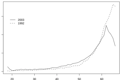
The corresponding age-specific inflows to disability are presented in Figure 2. Clearly, there has been a large decrease in the inflow rates for the oldest groups due to the AFP early pension scheme that was rolled out during this period, with lower age limit 62, see Røed and Haugen (2003) for details. There has also been an increase in the inflows for younger groups, more modest in absolute terms. The changes in inflow rates have not been particularly smooth however, as seen from the times series of aggregate inflows in Figure 3. The changes in inflow rates are explained partly by a temporarily stringent screening scheme for disability in the beginning of the 1990s, followed by reliberalisation later in the 1990s and presumably also effects of changing capacity in the administration of the benefits. There does not seem to be a close connection between the business cycle and
20 30 40 50 60 0.00 0.02 0.04 0.06 age
inflow to disability / population not on disability at start of period
2003 1992
Figure 2: Age specific annual inflow rates to disability. Men in Norway, 1992 and 2003
inflow rates to disability over time.
Individual disability pensions are calculated based on a rather complex scheme, de-scribed in more detail in Appendix A. The income dependent part of the disability ben-efits, the supplementary allowance, depends in a complex fashion on individual earnings histories, which for disabled persons include computed future earnings until age 66. 40 years of sufficiently high annual earnings are required for full pension rights. No credit is given for earnings prior to 1967. Hence, a person born in 1939 that enters the disability pension program can at best have 39 years of sufficiently high earnings, from 1967 until 2005, the year he becomes 66 years. Persons from later birth cohorts can have 40 years of sufficiently high earnings. Persons born in 1936 or earlier are covered by a rule that states that the number of years of earnings should be compared not with 40 years, but their number of potential years, which also covers the ages 67, 68, and 69, where no credit is derived for disability pensioneers.
For the purposes of the following discussion, I will condition on individual earnings his-tories. Exogeneity of individual earnings histories is however not a necessary assumption in the further analysis. When becoming disabled, benefits are computed based on the earn-ings history, transformed into a history of pension points at the NIS administration, with the consequence that earnings are in practice corrected for average wage growth. When
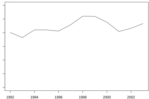
1992 1994 1996 1998 2000 2002 0.000 0.002 0.004 0.006 0.008 0.010 0.012 year transition rates
Figure 3: Inflow rate to disability for Norwegian men aged 18-66 years. 1992-2004
claiming that disability benefits depend on birth cohort, the counterfactual comparison is with a person becoming disabled at the same age, but one year earlier, with the same earnings history measured as earnings corrected for average wage growth. The main key to the variation is that it is impossible to earn pension points before 1967. In addition it is necessary to keep in mind that there is no gain from increasing the number of years with pension points beyond 40, and to keep in mind the denominator in equation (1), which is a strict function of birth cohort. DefineZ as a function of birth cohortc by
Z(c) = min(c−1900,40)
min(c−1897,40). (1)
A consecutive earnings history from age 27 until disablement is sufficient for Z(c) to de-scribe the correct relationship between birth cohort and the supplementary allowance, in the sense that individual benefits will be linear functions of Z(c), with both intercept and slope being individual specific. The intercept is then the earnings history independent part of the disability benefits and the slope is the supplementary allowance given full pension rights. A person from the 1940 birth cohort or later cohorts does not need any pension points from before age 27 to achieve full pension rights, as long as he has a consecutive earnings history from age 27 until disablement. On the other hand, persons from birth
cohorts 1939 and earlier could not earn any pension points before age 27.
For three reasons, the exposition above is too simple. First, there was a minor pension reform in 1992, leaving years with pension points before 1992 more valuable than years with pension points after 1992. Persons from later cohorts are less likely to have full set of pension years before 1992. However, the effects of this reform are very small. Five pension years missing before 1992 compensated by five years after 1992 leads to a reduction in the income dependent allowance of less than one percent. Hence I disregard this effect in the following.
Secondly, and importantly, many persons are covered by defined benefits occupational disability insurance schemes. In such schemes, the annual benefits are typically guaranteed to equal a certain proportion of the earnings at the time of the disabling event. The insurance company, or government in the case of public occupational schemes, contributes what is not already covered by the NIS scheme. The effect of the phasing in of the NIS scheme is then neutralised for those who are covered by such schemes. In practice, all public sector employees are covered by occupational disability insurance schemes. I do not have information about the degree of coverage in the private sector. While I cannot identify who are eligible for occupational pensions for the population at risk for disability, I am able to identify whether those who become disabled receive occupational pensions.
Finally, not everyone has earned pension points continuously from 1967 and until a disabling event. For persons with earnings histories deviating from this model, the rela-tionship between birth cohort and benefits is not correctly described byZ(c). E.g. for a person missing one year of pension points, but having an earnings history which could gen-erate pension points at age 26, the relevant relationship is similar toZ(c), but increasing in birth cohort until 1941. Each such nonlinear relationship should conceptually have been included in the empirical model below. However, a majority of the persons in our sample do in fact have consecutive earnings histories and each of the other nonlinear relationships between birth cohort and benefits affect only a very small minority of the sample.
3
Data
The data used here are stocks and flows in disability in Norway, based on the Fd-trygd database in Statistics Norway, covering the full data from the NIS, as well as demographic and income-related data. The full counts of residents in Norway for the cohorts discussed above is used, for the period 1992-2004. This gives good coverage for the most important
period with respect to disablement for the birth cohorts around the crucial 1937-1940-cohorts. 1992 1994 1996 1998 2000 2002 2004 0.16 0.18 0.20 0.22 0.24 year
share of population on disability rolls
60 years 59 years 58 years
Figure 4: Disability uptake rates, 1992-2004, for 58-, 59- and 60-year olds. The 1937 and 1940 birth cohorts marked.
Figure 4 demonstrates why it is not a good idea simply to study the share of the population that is disabled at a given age for the different birth cohorts, by plotting age specific disability uptake for three relevant ages versus year. While the graph for the 60 year olds seems consistent with a positive effect ofZ(c), giving an increase in benefits uptake for the years corresponding to the 1937-1940 birth cohorts, together with a general decreasing trend, the other graphs do not. The reason for the noisy appearance of the stocks is the short term variation in the inflows to disability seen in Figure 3 that contaminates the stocks, leaving the graphs in Figure 4 incomparable at a fine level. E.g. all stocks are high in the aftermath of the high inflow rates to disability in the late nineties. All stocks are also high in the early nineties.
To be able to control for the fluctuations in inflows, I study transition rates to disability with explicit year controls. Such transitions are studied over the years 1992-2004, with eleven annual transitions. Further, I only study transitions to disability for the ages 52-60 (in the starting year). Older workers’ inflow rates would presumably be strongly affected by the AFP early pension scheme, while the inflow rates among younger workers have also
Table 1: Descriptive statistics
Full sample 52 in ’92 52 in ’03 60 in ’92 60 in ’03 Number of persons 2589068 21592 29797 18604 24549 Share at risk 0.860 0.908 0.898 0.765 0.798 Subshare with CEH35a
0.841 0.867 0.833 0.851 0.832 Disability entrants 47301 212 340 544 697 Share of population 0.0183 0.0108 0.0127 0.0382 0.0355 Subshare with CEH35 0.740 0.750 0.682 0.814 0.773 Subshare with OPb
0.442 0.307 0.350 0.447 0.509 Subshare with CEH35, w/o OP 0.332 0.429 0.368 0.397 0.308
a
Consecutive earnings history of at least 1 times the NIS basic amount from age 35 up to 5 years before current date.
b
Occupational pensions exceeding 0.25 times the NIS basic amount, the year after inflow to disability.
changed quite a bit over this period. In addition, the 51-year olds in 1992 were from the 1941-cohort, hence there would be no variation in Z(c) for the 51 year olds. There is no extra variation inZ(c) generated by including the last years of data in the analysis either, as in 2003, persons from the 1943 to the 1951 birth cohorts are covered, so the inclusion of the last years only contribute indirectly by increasing the efficiency of nuisance parameter estimates. An important reform was implemented in 2004 creating a new disability benefit program in Norway, so later data are not included. Since individual characteristics except for age are not explicitly studied, the main dataset is essentially a year/age-matrix of numbers of persons at risk and the number who transit to disability.
Table 1 gives descriptive statistics for the full sample and the corners of our age/time matrix of transitions. Those at risk for disability are those not already covered by dis-ability benefits. From the second row in Table 1, it can be deduced that the share of the population on disability rolls increases with age from about 10 percent for 52 year olds to about 22 percent for 60 year olds, in consistency with Figure 1. The age structure in disability is clearly changing over the period studied, with disability uptake increasing for 52 year olds and decreasing for 60 year olds. The subshare of the population at risk that has a consecutive earnings history going back from 5 years before the risk for transition to age 35 is about 85 percent. The consecutive earnings history back to age 35 is measured because this can be done consistently for all birth cohorts. Years without pension points in the last five years prior to receipt of disability pensions are not taken into account, as such years are not likely to lead to lower pensions through Z(c) because they are likely to be related to the disabling event. The share of the population at risk that transits to disability is about 1 percent for the 52 year olds increasing to 3 percent for the 60 year
olds. The subshare with a consecutive earnings history is somewhat lower among those who transit to disability than for the full population at risk. The subshare of those who transit to disability with occupational pensions is somewhat under half, increasing in age and increasing over time. Whether a person qualifies for occupational pensions is mea-sured through the income register the year after the transition to disability. Occupational pensions beyond a certain minimum level, 0.25 times the NIS basic amount, are required to be classified with occupational pensions. Very small amount of occupational pensions are most likely not in practice defined benefits schemes that neutralize the effect ofZ(c). The subshare of those who transit to disability who has both a consecutive earnings history and does not have occupational pensions is about one third. Persons outside this group should not be affected by Z(c). Persons in this group should be affected by Z(c), except for the incovenient but small group with a consecutive earnings history going back to age 35, but not back to age 27.
4
The model and empirical results
The actual process of applying for and being considered eligible for disability benefits is rather messy, with requirements for being allowed to apply, processes for reapplication in the case of rejection etc. Still, one may hope that the main process is captured in the following simple conceptual framework: First, a negative health event occurs that makes a person eventually eligible for disability pension and the person knows this. Secondly, a person decides whether to take up the route leading to disability pensions. The choice of whether to take up disability pensions, conditional on eligibility, is a classic economic choice problem, depending on the utility if taking up disability pensions and the utility if staying outside the program. In addition to any psychological costs of program par-ticipation, the main cost of taking up disability is the limitation set to labour income or labour activity. Whatever other factor may be important for the choice, the income as a program participant and the income outside are plausible determinants of these utilities. The ambition in this paper is to measure the effects of the size of the disability benefit on this choice.
While it is not necessarily too difficult to set up a structural discrete choice model with benefits and labour income (implicitly) entering the utility function in a random utility framework, it is not clear how explicitly specifying such a model helps with the main identification problem: How do we find variation in benefit level generated by variables
that do not and are not correlated with unobserved variables that do affect disability uptake through other mechanisms?
The approach taken here is to model the probability of becoming eligible for disability pensions and taking up such pensions, and try to measure the effects of disability pension on this probability. This is done within the framework of a log-linear probability model. The reason for choosing this framework is that the model fits the data very well and that the parameters are interpretable as elasticities. The constructed variable logZ(c) is used as an instrumental variable to capture the effects of disability benefits. The essential assumption is that there are not other important nonlinear birth cohort effects that generates any apparent effect of logZ(c) on transition probabilities.
Our theoretical model is a binomial model with individual transition probabilities pi
fori= 1, . . . , n, given by
pi= exp(xiβi+ziγi), (2)
wherexiare vectors of covariates,zi = logZ(ci), whereciis the birth cohort of individuali, βiare vectors of individual specific nuisance parameters andγiare scalar individual specific
parameters of interest. The heterogeneity in parameters across individuals is important in the following because logZ(c), by hypothesis, should affect some of the persons in the sample but not others. The estimated model is of the form
pi = exp(xiβ+ziγ) (3)
However, when thepi’s are small numbers, as in this application, the maximum likelihood
estimate ˆγbased on the misspecified model in equation (3) can be interpreted as an estimate of the weighted average over individual γi, with weights proportional topi, in addition to
the squared covariate values that constitute such weights in a linear model. To be precise, let ˆγ∗ denote the limit of ˆγ as the number of observations goes to infinity. Now,
ˆ γ∗ ≈ P piz˜i2γi P ˆ piz˜i2 , (4)
where ˆpi are the estimated probabilities from the misspecified model and ˜zi is zi cleansed
of variation that can be expressed as a linear function of other covariates in the precise sense of ˜ zi=zi−( n X j=1 ˆ pjxjx0j)−1( n X j=1 ˆ pjxjzj0). (5)
See Appendix B for a further discussion.
Our main parameter of interest is not the elasticity of transitions probabilities with respect to Z(ci), but rather the elasticity with respect to benefit level,Bi, which I denote . Assume that is the same for everyone, so that the heterogeneity in the elasticity of transition probabilities with respect to Z(c) is only due to differences in the elasticity of
Bi with respect toZ(c). Then
γi = ∂logBi ∂logZ(ci) (6) Hence, ˆ γ∗ ≈ Pn i=1piz˜2i ∂logBi ∂logZ(c) Pn i=1pˆiz˜i2 , (7)
which can neatly be approximated by ˆγ ≈ν, where
ν= m X i=1 ˜ z2ji ∂logBi ∂logZ(c)/ m X i=1 ˜ zj2i, (8)
wherej1, . . . , jm are the indices of those who transit to disability. Thus,ν can be
approxi-mated by a weighted averageamong those who become disabled, with weights based on the squared cleansed covariates ˜zi2. Thus, the estimate of the elasticity of interest is found by ˆ
≈γ/νˆ , whereν is possible to compute in our data.
In a more general setting, the elasticity of interest is also heterogeneous, and then
n−1X i wi ∂logpi ∂logBi ≈ γˆ ν, (9) where wi=piz˜i2 ∂logBi ∂logZ(c)/ X i ˆ piz˜2i ∂logBi ∂logZ(c). (10)
Hence, the estimate of the elasticity may be interpreted as a local average effect, weighted both by the probability of transition to disability, the effect of the nonlinear cohort effect
Z(c) on benefits and on the squared cleansed covariates. Keeping this interpretation in mind, I will in the following refer to this parameter as ”the elasticity”.
With the covariates used below, the difference between the approach taken here and a simple approach studying the full transition probability to disability in the age range 52-60 years is that I (i) can control for the fact that different birth cohorts were faced with years with different disability uptake probabilities, (ii) can use cohorts for which I do not have data for all the transitions and (iii) can take into account smoothly changing age structure
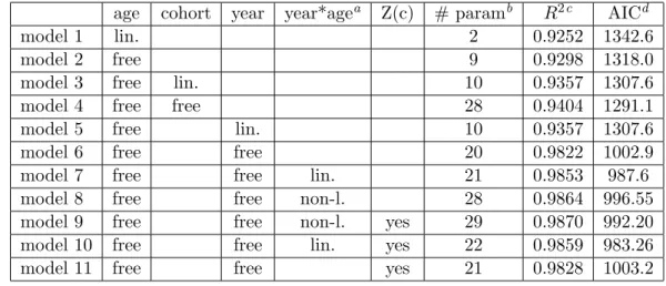
Table 2: Goodness of fit of different model specifications. age cohort year year*agea
Z(c) # paramb
R2c
AICd
model 1 lin. 2 0.9252 1342.6
model 2 free 9 0.9298 1318.0
model 3 free lin. 10 0.9357 1307.6 model 4 free free 28 0.9404 1291.1 model 5 free lin. 10 0.9357 1307.6 model 6 free free 20 0.9822 1002.9 model 7 free free lin. 21 0.9853 987.6 model 8 free free non-l. 28 0.9864 996.55 model 9 free free non-l. yes 29 0.9870 992.20 model 10 free free lin. yes 22 0.9859 983.26 model 11 free free yes 21 0.9828 1003.2
a
Nonlinear interaction effect between year and age should be interpreted as age-specific linear trends.
b
The relevant sample size is for comparison 117.
c
R2 based on linear model approximation.
d
Akaike’s information criterion based on exact model.
in the transitions to disability over time. Still, the reader may prudently worry that the results obtained are sensitive to the exact model specification. Indeed, since any such model is at best only an approximation to the real underlying process, one may worry that the nonlinear cohort effects reflect model misspecifications rather than changing benefit levels. The first reply to this objection is to demonstrate that the model fits the data very well.
Table 2 provides evidence of the model fit and how it is affected by the inclusion of various variables. Model fits are assessed by making a linear model approximation, simply using the log transition rate for each cell as dependent variable. The basis for this approximation is the standard Gaussian approximation to the binomial, dating back to de Moivre. The linear model approximation is only used for generating the R2-numbers in Table 2.
Most of the variance in the age/year - cell specific log transition rates can be explained by age. The log transition rate is close to linear in age, though a free specification, with a separate parameter for each age, improves the model fit (enough to be clearly statistically significant at standard levels). This is the right point to study cohort trends because cohort trends will later be picked up by the year effects. Including a linear cohort trend improves the fit of the model and gives a weak positive trend over time. Including cohort specific fixed effects improves the model further. However, the fit of the model is much better if there are year specific fixed effects in the model, even though there are only 11 years compared to 19 cohorts. Model 5 with linear year effects is equivalent to model 3 with
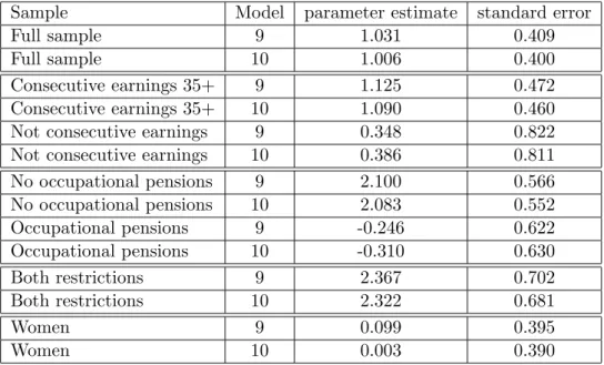
Table 3: Point estimates from Models 9 and 10 of the parameter associated with Z(c). Full sample and partitioned samples
Sample Model parameter estimate standard error
Full sample 9 1.031 0.409
Full sample 10 1.006 0.400
Consecutive earnings 35+ 9 1.125 0.472 Consecutive earnings 35+ 10 1.090 0.460 Not consecutive earnings 9 0.348 0.822 Not consecutive earnings 10 0.386 0.811 No occupational pensions 9 2.100 0.566 No occupational pensions 10 2.083 0.552 Occupational pensions 9 -0.246 0.622 Occupational pensions 10 -0.310 0.630 Both restrictions 9 2.367 0.702 Both restrictions 10 2.322 0.681 Women 9 0.099 0.395 Women 10 0.003 0.390
linear cohort effects. The reason for the improvement when taking into account year effects compared to cohort effects is that the year effects are highly nonlinear, starting out rather low, increasing to a top around 1999 and then decreasing again, as seen in Figure 3. In fact, after controlling for year effects, very little of the original variability is left. However, the model can and should still be improved by introducing an interaction term between age and year. Free age specific linear year trends do not give a substantial improvement over a simple linear interaction term, though results for both specifications are reported in the following, as the model with more parameters is most likely more robust. Including logZ(c) gives a statistically significant improvement of the model at the 0.05 level. The p-values based on likelihood ratio tests, computable from the reported AIC-values, are 0.007 for both model 9 and model 10, compared to model 8 and model 7, respectively.
The weighted average elasticity of benefits with respect to logZ(c),νfrom equation (8), is in our data computed to 0.23. The computation is based on the share of the individual benefits received that are supplementary allowances. In addition, at the individual level, the elasticity of benefits to logZ(c) is set to zero if the person in question is registered with occupational pensions or without a consecutive earnings history. The weights in the weighted average differ substantially across age-year cells. However, the within-cell averages of the measured elasticity do not differ much across cells. The unweighted average is about 0.22.
of transitions to disability with respect toZ(c) of about 1 together with the computed value of ν imply that the point estimate of the elasticity of transitions to disability on benefits levels is about 4.5. This is at face value a quite high elasticity. It is measured with considerable uncertainty as seen from the standard error in Table 3. The lower limit of a 95 percent (Wald) confidence interval is slightly above 1, which is still reasonably high.
The critical reader will still worry that the nonlinear cohort effects through logZ(c) picks up something else than changes in disability benefits. The second answer is to provide robustness tests that corroborate the hypothesis that the nonlinear cohort effects indeed mainly pick up the effects of changing benefit levels.
The first robustness test is to estimate the model separately for two partitions of the sample, with the partioning based on whether the individuals have consecutive earnings histories back to age 35, the strictest I am able to measure consistently for all cohorts. The estimates based on the restricted sample without those missing a consecutive earnings history should on one hand give better estimates than the original ones, because a number of persons who could potentially have nonlinear effects of cohort that differs from Z(c) are left out. On the other hand, using selected samples naturally introduces selection problems. It is clear from Table 1 that the proportion, both of the population at risk and among those who transit to disability, is changing over time. Such selection problems can be expected to be of two variants. First, as indicated, the proportions change over time, which probably means that the distributions of transition probabilites within each sample partition changes over time. Secondly, even if the proportion had been constant, different types of persons could be expected to satisfy the sample selection criteria, conditional on cohort. As should be clear from the main identifying mechanism in this paper, the incentives to secure a consecutive earnings history are cohort dependent. Still, assuming that these effects are small or can be captured by the linear cohort trend in our models, the effect ofZ(c) on the selected sample should be stronger and the effect ofZ(c) on those sorted out should be about zero. As is seen from rows 3-6 in Table 3, the effect of Z(c) increases somewhat when the sample is limited to only those with a consecutive earnings history. Importantly, a small and statistically insignificant estimate of the effect ofZ(c) is associated with those without a consecutive earnings history.
In addition, I do a similar, but not identical, robustness test based on those who qual-ify for occupational pensions. Note first that this sample selection would create similar problems as above. However, in addition, I do not know upfront the proportion in the
population at risk who qualify for occupational pension, only the proportion who qualify for occupational pension among those who become disabled. It is still possible to estimate separate models based on the numbers transiting to disability with occupational pensions and those who transit to disability without occupational pensions. The same population at risk can be used for both these estimation exercises. There are two points to make about this. First, the likelihood of the binomial distribution is about the same for events with small probability, independent of whether the population at risk is changed. More precisely, halving the population at risk size and doubling the transition probability leaves the likelihood more or less unchanged. Thus, in the absence of changing proportions with occupational pensions and sample selection problems, not knowing which part of the pop-ulation is at risk for which type of transition is not problematic. However, the proportions do change over time. If, however, the controls are able to pick up the changing effective numbers at risk given sample partition, as above, the effects ofZ(c) on the transitions to disability without occupational pensions should be stronger than the original estimate and the effects of Z(c) on the transitions to disability with occupational pensions should be zero. From Table 3, the effect of Z(c) increases strongly when only transitions to disabil-ity without occupational pensions are studied. There is a small negative and statistically insignicant effect of Z(c) on transitions to disability with occupational pensions. When both restrictions are imposed the effect ofZ(c) is even stronger. There are no appreciable differences between Model 9 and Model 10.
The observant reader will now notice that it is possible to compute a difference-in-difference estimator, with those with occupational pensions as a control group and the doubly restricted sample as a treatment group. I argued above that I prefer the instru-mental variable estimator above to the difference-in-difference version, because the latter involves stronger assumptions related to the ability of the controls to capture the effects of sample selection. However, for the reader who disagrees, the other estimate is supplied. The relevant difference-in-difference estimate of the effect of logZ(c) is then 2.6 for model 9, with a standard error of 0.94. When this is translated into the elasticity with respect to benefits, the point estimate is about 3.8. (Theν in this computation is based only on those in the restricted sample.) The fact that the estimation results are qualitatively the same should not be seen as independent verification of the robustness because the estimates are based on essentially the same information. The estimates would differ if the effect of logZ(c) on the control group was substantially different from zero.
The third robustness test is to replicate the analysis with women rather than men. Very few women in these age groups have the consecutive earnings history required to make Z(c) matter. The relevant share of the disabled women with a consecutive earnings history back to age 35 and without occupational pensions is 11,7 percent. However, even this small number overestimates the share that would be affected byZ(c) because most of these women are from birth cohorts after 1940. The hypothesis is then that the effect of
Z(c) on women should be close to zero, which it indeed is.
Why have I left out standard explanatory variables such as education, work experience etc? If we believe that there is an initial distribution that is determined at an early stage (early childhood) that has an impact on later probabilities of health shocks, this variable is most likely interrelated with later achievements such as education, family situation, work experience etc. Hence, if e.g. there is a strong relationship between educational level and propensity to become disabled within a cohort, we should not necessarily conclude that there should be changing propensity to become disabled due to changing education levels, because there will be an element of sorting. The same argument would apply to more or less any explanatory variable except gender and age. This is not a general argument for why I could not have included individual covariates as controls in the model - it is an argument for why uncorrected cohort effects may be as good as cohort effects with individual characteristics netted out. Leaving individual characteristics out of the analysis also allows for a stronger focus on the goodness of fit of the model as a model predicting disability across age, time and cohort.
5
Concluding discussion
The present paper demonstrates that transitions to disability for men in their fifties are increasing in benefit levels. The point estimates indicate very strong effects, but these should be interpreted with caution, as the confidence intervals also include more moderate values.
Taking point estimates at face value, however, the effects are much stronger than similar estimates based on data from Canada or the UK. I have two hypotheses for why elasticities should be higher in Norway than in most other countries. First, there should be a negative relationship between the stringency of the requirements for receiving disability function and the elasticity with respect to benefit levels. The ”marginal” disability pensioneer (with respect to stringency of requirement) should be more responsive to economic incentives
than the average disability pensioneer because the pool of pensioneers include a substantial number of persons that are so disabled that they are in practice not able to work. Relatively high disability uptake in Norway, not least for the age group studied here, indicates that the requirements for receiving disability benefits are not particularly stringent, compared to programs in other countries.
Secondly, it is not clear that the elasticity with respect to the benefits or the elasticity with respect to the replacement rates are the best parameterization of such effects. Indeed, basic economic theory would suggest that employment drops to zero for those who qualify for the programs as the replacement rate goes to one. Thus, one should expect high elasticities with respect to benefit level for countries with high replacement rates. Norway is characterized by very high replacement rates, not least net replacement rates for disability pensioneers, who often earn small supplementary allowances. Net replacement rates are about 60 to 70 percent for the typical pensioneer studied here. Thus, a 1 percent change in benefits will lead to a change in the difference between net income inside and outside the program of about 2 percent.
The results provided here are of policy relevance for at least two reasons. First, they show that there are important incentive problems associated with the disability pension program. If the disability benefits had been lower, more persons would have stayed out of the program, plausibly to participate in the labour market instead. Hence, there is a substantial element of choice in the transitions to disability pensions. In boldface, the results provided here are a strong indication that the disability pension program in Norway constitutes a large scale waste of resources through subsidising voluntary early withdrawal from the labor force. This is quite likely at odds with the aims of the program. Secondly, substantial effects of benefits on transitions to probability mean that increases or decreases in benefits will have important effects on the fiscal costs of benefit programs not only directly, but also indirectly, through affecting behaviour. This is of current policy relevance, as the benefits for the disabled are about to be revamped as part of a larger reform of the Norwegian pension system.
References
Andreassen, L., and T. Kornstad (2006): “Hvorfor g˚ar flere fra sykemelding til uførhet?,” Tidsskrift for velferdsforskning, 9(3), 126–147.
Autor, D.,andM. Duggan(2006): “The Growth in the Social Security Disability Rolls: A Fiscal Crisis Unfolding,” Journal of Economic Perspectives, 20(3), 71–96.
Bell, B., andJ. Smith(2004): “Health, disability insurance and labour force participa-tion,” Working Paper 218, Bank of England.
Bound, J. (1989): “The Health and Earnings of Rejected Disability Insurance Appli-cants,”American Economic Review, 79(3), 482–503.
(1991): “The Health and Earnings of Rejected Disability Insurance Applicants: Reply,” American Economic Review, 81(5), 1427–1434.
Bowitz, E. (1997): “Disability benefits, replacement ratios and the labour market. A time series approach,” Applied Economics, 29(7), 913–923.
Bratberg, E. (1999): “Disability Retirement in a Welfare State,”Scandinavian Journal of Economics, 101(1), 97–114.
Campolieti, M. (2004): “Disability Insurance Benefits and Labor Supply: Some Addi-tional Evidence,” Journal of Labor Economics, 22(4), 863–889.
Chen, S., and W. van der Klaauw (2008): “The work disincentive effects of the disability insurance program in the 1990s,”Journal of Econometrics, 142(2), 757–784.
Gruber, J.(2000): “Disability Insurance Benefits and Labor Supply,”Journal of Political Economy, 108(6), 1162–1183.
Haveman, R. H., and B. L. Wolfe(1984): “The Decline in Male Labor Force Partici-pation: Comment,”Journal of Political Economy, 92(3), 532–541.
Holen, D. S.(2007): Disability Pension in Norway. Ph.D. dissertation.Faculty of Social Sciences, University of Oslo.
Imbens, G. W., and T. Lemieux(2008): “Regression discontinuity designs: A guide to practice,” Journal of Econometrics, 142(2), 615–635.
Parsons, D. O. (1980): “The Decline in Male Labor Force Participation,” Journal of Political Economy, 88(1), 117–134.
(1991): “The Health and Earnings of Rejected Disability Insurance Applicants: Comment,” American Economic Review, 81(5), 1419–1426.
Røed, K.,andF. Haugen(2003): “Early Retirement and Economic Incentives: Evidence from a Quasi-natural Experiment,” Labour, 17(2), 203–228.
Rege, M., K. Telle, and M. Votruba (2005): “The effect of plant downsizing on disability pension utilization,” Discussion Paper 435, Statistics Norway.
(2007): “Social Interaction Effects in Disability Pension Participation: Evidence from Plant Downsizing,” Discussion Paper 496, Statistics Norway.
A
Calculation of disability benefits in Norway
The disability pension scheme is tightly integrated into the old age pension scheme. The old age pension consists of a basic allowance and a supplementary allowance. If this sum does not exceed a small limit, the sum of the basic allowance and a special supplement is granted instead (the minimum pension). The basic allowance depends on whether a person is single or married and the number of years of residence in Norway, but not on previous earnings. The supplementary allowance depends on the earnings history. In addition to these allowances, there are special allowances for persons with dependents.
The ”currency” in the NIS pension system is G, the ”basic amount”. A low wage annual income is about 4 G. G is adjusted somewhat ad hoc, but still more or less in line with the average wage growth in Norway. Since 1967, a person has been awarded annual pension points for earnings in excess of 1 G. When the old age pension is calculated, a persons full pension point history is taken into account. It is possible to earn pension points up to age 69. The supplementary allowance measured in G can be described as the product of three factors.
The first factor depends on the number of years of non-zero pension points. For younger cohorts, this factor equals the ratio of the number of years on non-zero pension points to 40 years, with no credit for years in excess of 40. For older birth cohorts, the number of years of non-zero pension points is compared with the maximum possible number of pension points years, equal to the number of years from 1967 until and including the year they became 69 years old, rather than with 40 years.
The second factor is the average of the best 20 years of pension points, or the average of all years with nonzero pension points if there are fewer than 20 years of non-zero pension points.
The third factor is 0.45 times the proportion of pension points before 1992 and 0.42 times the proportion of years of pension points from 1992 onwards. Only 40 years are taken into account, with excess years shaved off the number of years after 1992.
When a person is granted disability pension, a date is set for the disabling event. This will typically be the date when the person started receiving sickness benefits, but could also be set earlier than this. The future computed earnings can then be generated. This is the best of the average of the three years immediately prior to the year including the disabling event and the average of the best half of the years with non-zero pension points. A person is then granted future earnings (in G) equal to the future computed earnings every year up to and including the year the person becomes 66 years. If a person does not earn more pension points, the disability pensions will then be constant until retirement age and then be replaced by old age pensions with exactly the same benefit level.
B
The theory of loglinear probability models with
hetero-geneous coefficients
This appendix describes some properties of the loglinear probability model in the interest-ing case where the parameters of the model vary within the population studied, while the estimated model is specified with homogeneous parameters.
The loglinear probability model can be expressed as a binomial model where the prob-ability pi depends onxi through the equation
pi= exp(xiβ). (11)
The loglinear probability model is deficient in the sense that it can generate ties that exceed 1. This is not a relevant problem when we study limits as probabili-ties go to zero. Indeed, the results presented here hold for the complementary log-log probability model (pi = 1 −exp(exp(xiβ))) and for the logit probability model (pi =
exp(xiβ)/(1 + exp(xiβ))). Both these models approximate the loglinear probability model
when probabilities go to zero, that is, when xiβ → −∞.
The log-likelihood function of the loglinear probability model is
l(β) =X
i
whereyi takes on the value 1 upon success, 0 otherwise. The score function is
S(β) =∂l/∂β=X
i
yi−exp(xiβ)
1−exp(xiβ)xi, (13)
and the Fisher information matrix is
I(β) = ∂ 2l(β) ∂β2 = X i (yi−1) exp(xiβ) (1−exp(xiβ))2 xix 0 i, (14)
Assume that yi results from a different model, whereβ are individual specific βi, thus
the true model is characterized by pi = exp(xiβi). We will now see how the maximum
likelihood estimate of β depends on the individual βi. Such changes affect the likelihood
trough yi.
Substitute exp(xiβi) foryi in the score function. This is only sensible in a large sample
setting. As a very strict variant, there are only a finite number of values of xiβi and each
of these occur infinitely often as n→ ∞. The expected score function is now
E(S(β)) =X
i
exp(xiβi)−exp(xiβ)
1−exp(xiβ) xi, (15)
The limit of the ML estimate ˆβ is implicitly found by E(S( ˆβ)) converging to zero as
n→ ∞.
Hence, the effect of βi on the (limit of the) ML estimate ˆβ can be found through
differentiation as ∂βˆ ∂β1 =−(I(β))−1∂E(S(β)) ∂β1 (16) with ∂E(S(β)) ∂β1 = expxiβ 1−exp(xiβ)x1x 0 1, (17)
Thus, as exp(xiβi) goes to zero for alli, (formally e.g. by letting allxiβi contain a common
intercept term that goes to−∞,)
∂βˆ ∂β1 =−( X i ˆ pixix0i)−1p1x1x01 (18)
In a linear, as opposed to loglinear, probability model, as in other types of linear model, the least squares estimate can be expressed as weighted average of individual coefficients, where the weights are squared covariates, as in the equation above. However, in the case of the loglinear probability model, the choice probabilities also enter the weights. In addition,
of course, the ML estimate is not a weighted average. However, if we write ˆβ, approximated as a linear function of βi, the coefficients will sum up to approximately one, if pi and ˆpi
do not differ too much.
Based on equation (18), it seems reasonable to assume that the limit of the maxi-mum likelihood of the estimated β will approximate a probability weighted average over individual βi, as long as the distribution of the covariates is independent ofβi.
Sometimes, it may be necessary to take into account a systematic relationship between covariates andβi. This is the case in this paper, where the distribution of the elasticity of Bi on Z(ci) must be expected to vary with ci.
It is necessary to be careful when interpreting the contribution of xi to the weights in
the multivariate case. The formula includes the inverse of the (misspecified) probability weighted covariance matrix of X, the matrix of stacked individual covariates. The effect of one scalar parameter in the process generating the data on one scalar parameter in the (limit of the) ML estimate is a linear product. Our focus is on a scalar parameter of interest. It is possible to derive the relationship between the distribution of the true parameter of interest and the scalar estimate of the parameter of interest, through linear operations on the matrix X.
1. Compute ˆpi from the estimated loglinear probability model.
2. Estimate the weighted least squares regression, with ˆpi as weights, of the variables
associated with the nuisance parameters on the variable associated with the parameter of interest.
3. Substitute the residuals from this analysis for the variable associated with the param-eter of interest in the vectorsxi.
Clearly, a reanalysis with the new covariate vector will give exactly the same estimate of the parameter of interest, although the nuisance parameters will change. The matrix
P
ipˆixix0i now have zero entries on the off-diagonal elements in the row and column
asso-ciated with the parameter of interest. The same holds true when the matrix is inverted. Hence, the weights in equation (18) can be interpreted as in the case of scalar parame-ters, as long as the variable associated with the parameter of interest is first ”cleansed” of variation that can be expressed as a linear combination of the control variables.