Hydrologic Modeling System HEC-HMS

(1)

Hydrologic Engineering Center



Hydrologic Modeling System

HEC-HMS

User's Manual

Version 4.0

(2)

REPORT DOCUMENTATION PAGE

_{OMB No. 0704-0188} Public reporting burden for this collection of information is estimated to average 1 hour per response, including the time for reviewing instructions, searching existing data sources, gathering and maintaining the data needed, and completing and reviewing the collection of information. Send comments regarding this burden estimate or any other aspect of this collection of information, including suggestions for reducing this burden, to Washington Headquarters Services, Directorate for Information Operations and Reports, 1215 Jefferson Davis Highway, Suite 1204, Arlington, VA 22202-4302, and to the Office of Management and Budget, Paperwork Reduction Project (0704-0188), Washington DC 20503.

1. AGENCY USE ONLY (Leave Blank) 2. REPORT DATE

December 2013

3. REPORT TYPE AND DATES COVERED

Computer Software User's Manual

4. TITLE AND SUBTITLE

Hydrologic Modeling System HEC-HMS User's Manual

5. FUNDING NUMBERS

6. AUTHOR(S)

William A. Scharffenberg

7. PERFORMING ORGANIZATION NAME(S) AND ADDRESS(ES)

U.S. Army Corps of Engineers Hydrologic Engineering Center, HEC 609 Second St.

Davis, CA 95616

8. PERFORMING ORGANIZATION REPORT NUMBER

9. SPONSORING / MONITORING AGENCY NAME(S) AND ADDRESS(ES)

HQ U.S. Army Corps of Engineers 441 G St., NW

Washington, DC 20314-1000

10. SPONSORING / MONITORING AGENCY REPORT NUMBER

11. SUPPLEMENTARY NOTES

12A. DISTRIBUTION / AVAILABILITY STATEMENT

Distribution is unlimited.

12B. DISTRIBUTION CODE

13. ABSTRACT (Maximum 200 words)

The Hydrologic Modeling System (HEC-HMS) is designed to simulate the complete hydrologic processes of dendritic watershed systems. In includes many traditional hydrologic analysis procedures such as event infiltration, unit hydrographs, and hydrologic routing. It also includes procedures necessary for continuous simulation including evapo-transpiration,

snowmelt, and soil moisture accounting. Advanced capabilities are also provided for gridded runoff simulation using the linear quasi-distributed runoff transform (ModClark). Supplemental analysis tools are provided for parameter estimation, depth-area analysis, flow forecasting, erosion and sediment transport, and nutrient water quality.

The program features a completely integrated work environment including a database, data entry utilities, computation engine, and results reporting tools. A graphical user interface allows the user seamless movement between the different parts of the program. Simulation results are stored in the Data Storage System HEC-DSS and can be used in conjunction with other software for studies of water availability, urban drainage, flow forecasting, future urbanization impact, reservoir spillway design, flood damage reduction, floodplain regulation, and systems operation.

Program functionality and appearance are the same across all supported platforms. It is available for Microsoft Windows®, Oracle Solaris™, and Linux® operating systems.

14. SUBJECT TERMS

Hydrology, watershed, precipitation runoff, river routing, flood frequency, flood control, water supply, computer simulation, environmental restoration.

15. NUMBER OF PAGES 440 16. PRICE CODE 17. SECURITY CLASSIFICATION OF REPORT 18. SECURITY CLASSIFICATION OF THIS PAGE 19. SECURITY CLASSIFICATION OF ABSTRACT 20. LIMITATION OF ABSTRACT

(3)

Hydrologic Modeling System

HEC-HMS

User's Manual

Version 4.0

December 2013

US Army Corps of Engineers

Institute for Water Resources

Hydrologic Engineering Center

609 Second Street

Davis, CA 95616 USA

(4)

Hydrologic Modeling System HEC-HMS, User's Manual

2013. This Hydrologic Engineering Center (HEC) Manual is a U.S. Government document and is not subject to copyright. It may be copied and used free of charge. Please acknowledge the U.S. Army Corps of Engineers Hydrologic Engineering Center as the author of this Manual in any subsequent use of this work or excerpts.

Use of the software described by this Manual is controlled by certain terms and conditions. The user must acknowledge and agree to be bound by the terms and conditions of usage before the software can be installed or used. For reference, a copy of the terms and conditions of usage are included in Appendix E of this document so that they may be examined before obtaining the software.

This document contains references to product names that are used as trademarks by, or are federally registered trademarks of, their respective owners. Use of specific product names does not imply official or unofficial endorsement. Product names are used solely for the purpose of identifying products available in the public market place.

Intel and Pentium are registered trademarks of Intel Corp. Linux is a registered trademark of Linus Torvalds.

Microsoft and Windows are registered trademarks of Microsoft Corp. Vista is a trademark of Microsoft Corp.

RED HAT is a registered trademark of Red Hat, Inc.

Solaris and Java are trademarks of Oracle, Inc. UltraSPARC is a registered trademark of SPARC International.

(5)

PREFACE

XIII

INTRODUCTION

1

SCOPE ... 1

HISTORY ... 1

CAPABILITIES ... 2

Watershed Physical Description ... 2

Meteorology Description ... 3

Hydrologic Simulation ... 4

Parameter Estimation ... 4

Analyzing Simulations ... 5

Forecasting Future Flows ... 5

Sediment and Water Quality ... 5

GIS Connection ... 5 LIMITATIONS ... 5 Model Formulation ... 6 Flow Representation ... 6 DOCUMENTATION CONVENTIONS ... 7 REFERENCES ... 7

INSTALLING AND RUNNING THE PROGRAM

9

OPERATING SYSTEM REQUIREMENTS ... 9

HARDWARE REQUIREMENTS AND RECOMMENDATIONS ... 9

INSTALLATION ... 10

Microsoft Windows Operating System ... 10

Sun Microsystems Solaris Operating System ... 11

Linux Operating System ... 12

RUNNING THE PROGRAM ... 13

Microsoft Windows Operating System ... 13

Sun Microsystems Solaris Operating System ... 13

Linux Operating System ... 13

COMMAND LINE OPERATION ... 14

MANAGING MEMORY ALLOCATION ... 15

ADDITIONAL RESOURCES ... 15

OVERVIEW

17

PROGRAM SCREEN ... 17 Menu System ... 18 Toolbar ... 21 Watershed Explorer ... 21 Desktop ... 23 Component Editor ... 23 Message Log... 25 PROGRAM SETTINGS ... 25 DATA CONVENTIONS ... 26 Saving Properties ... 26 Number Formatting ... 27

Date and Time Formatting ... 27

Units Conversion ... 28

Interpolation ... 28

APPLICATION STEPS ... 29

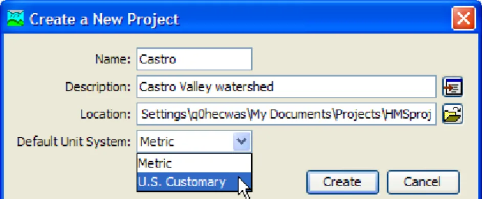
Create a New Project ... 29

(6)

Enter Simulation Time Windows ... 35

Simulate and View Results ... 36

Create or Modify Data ... 38

Make Additional Simulations and Compare Results ... 39

Exit the Program ... 39

REFERENCES ... 39

PROJECTS AND CONTROL SPECIFICATIONS

41

PROJECTS ... 41

Creating a New Project ... 41

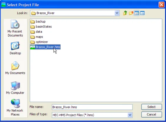
Opening a Project ... 42

Copying a Project ... 43

Renaming a Project ... 44

Deleting a Project ... 45

Project Properties ... 45

DIRECTORIES AND FILES ... 46

Files Generated by the Program ... 46

Files Specified by the User ... 47

Manually Entered Time-Series and Paired Data ... 48

Computed Results ... 48

External Time-Series, Paired, and Grid Data ... 48

Security Limitations ... 49

CONTROL SPECIFICATIONS ... 49

Creating a New Control Specifications ... 49

Copying a Control Specifications ... 50

Renaming a Control Specifications ... 51

Deleting a Control Specifications ... 52

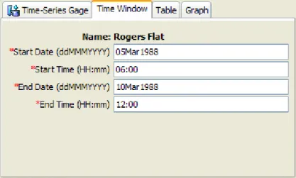
Time Window ... 54

Time Interval ... 55

Gridded Data Output Interval... 55

Grid Time Shift ... 56

IMPORTING HEC-1FILES ... 56

Selecting and Processing a File ... 57

Unsupported Features ... 58

REFERENCES ... 60

SHARED COMPONENT DATA

61

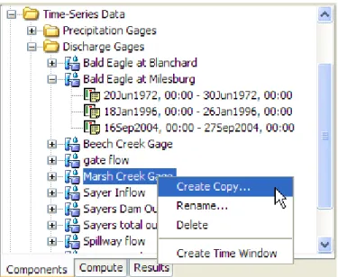
TIME-SERIES DATA ... 61

Creating a New Gage ... 61

Copying a Gage ... 62 Renaming a Gage ... 63 Deleting a Gage ... 65 Time Windows ... 66 Data Source ... 69 Data Units ... 70 Time Interval ... 70

Retrieval From a HEC-DSS File ... 71

Table ... 74

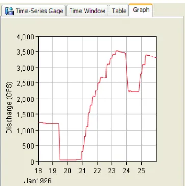
Graph ... 75

Latitude and Longitude ... 75

Elevation ... 76

Reference Height ... 76

PAIRED DATA ... 76

Creating a New Curve ... 76

Copying a Curve ... 77

(7)

Deleting a Curve ... 80

Data Source ... 81

Data Units ... 82

Time Intervals ... 82

Table ... 85

Graph ... 86

GRID DATA ... 87

Creating a New Grid ... 87

Copying a Grid ... 88

Renaming a Grid ... 89

Deleting a Grid ... 90

REFERENCES ... 97

WATERSHED PHYSICAL DESCRIPTION

99

BASIN MODELS ... 99

Creating a New Basin Model ... 99

Copying a Basin Model ... 100

Renaming a Basin Model ... 101

Deleting a Basin Model ... 102

Importing a Basin Model ... 103

BASIN MODEL PROPERTIES ... 104

Gridded Subbasins ... 104 Local Flow ... 104 Flow Ratio ... 105 Missing Flow ... 105 Unit System ... 105 Sediment ... 105 Water Quality ... 106 BASIN MODEL MAP ... 106 Background Maps ... 106 Maximum Extents ... 108 Background Gridlines ... 109

Adjusting the View and Zooming ... 109

Drawing Elements and Labels ... 110

Displaying Flow Directions ... 111

HYDROLOGIC ELEMENTS ... 111

Creating a New Element ... 112

Copying an Element ... 113

Pasting an Element ... 114

Cutting an Element ... 115

Renaming an Element ... 116

Deleting an Element ... 116

Optional Element Properties ... 118

Element Inventory ... 119

Finding and Selecting Elements ... 120

FLOW NETWORK ... 121

Moving Elements ... 121

Rescaling Elements ... 122

Locking Element Locations ... 122

Connecting and Disconnecting Elements ... 123

Hydrologic Order ... 125

(8)

Copying a Zone Configuration ... 130

Renaming a Zone Configuration ... 130

Deleting a Zone Configuration ... 131

Creating a Zone in a Configuration ... 132

Renaming a Zone in a Configuration ... 133

Deleting a Zone from a configuration ... 133

Adding Elements to a Zone ... 134

Removing Elements from a Zone ... 135

Selecting a Current Zone Configuration ... 136

COMPUTATION POINTS ... 139

Selecting Computation Points ... 139

Unselecting Computation Points ... 141

Selecting Calibration Parameters ... 143

Unselecting Calibration Parameters ... 145

Settings for Calibration Parameters ... 146

Computation Point Results ... 147

Using the Calibration Aids ... 149

REFERENCES ... 151

SUBBASIN ELEMENTS

153

SELECTING A CANOPY METHOD ... 153

Dynamic Canopy ... 154

Gridded Simple Canopy ... 155

Simple Canopy ... 156

SELECTING A SURFACE METHOD ... 157

Gridded Simple Surface ... 157

Simple Surface ... 158

SELECTING A LOSS METHOD ... 158

Deficit and Constant Loss... 159

Exponential Loss ... 160

Green and Ampt Loss ... 161

Gridded Deficit Constant Loss ... 161

Gridded Green and Ampt Loss ... 163

Gridded SCS Curve Number Loss ... 163

Gridded Soil Moisture Accounting ... 164

Initial and Constant Loss ... 165

SCS Curve Number Loss ... 166

Smith Parlange Loss ... 167

Soil Moisture Accounting Loss ... 168

SELECTING A TRANSFORM METHOD ... 169

Clark Unit Hydrograph Transform ... 170

Kinematic Wave Transform ... 170

ModClark Transform ... 174

SCS Unit Hydrograph Transform... 174

Snyder Unit Hydrograph Transform ... 175

User-Specified S-Graph Transform ... 178

User-Specified Unit Hydrograph Transform ... 178

SELECTING A BASEFLOW METHOD ... 179

Bounded Recession Baseflow ... 179

Constant Monthly Baseflow ... 180

Linear Reservoir Baseflow ... 181

Nonlinear Boussinesq Baseflow ... 182

Recession Baseflow ... 183

REACH ELEMENTS

185

SELECTING A ROUTING METHOD ... 185

(9)

Kinematic Wave Routing ... 186

Lag Routing ... 187

Modified Puls Routing ... 187

Muskingum Routing ... 188

Muskingum-Cunge Routing ... 189

Straddle Stagger Routing ... 190

SELECTING A LOSS/GAIN METHOD ... 191

Constant Loss/Gain ... 191

Percolation Loss/Gain ... 192

RESERVOIR ELEMENTS

195

SELECTING A ROUTING METHOD ... 195

OUTFLOW CURVE ROUTING ... 196

Storage Method ... 196

Initial Condition ... 197

SPECIFIED RELEASE ROUTING ... 197

Discharge Gage Selection ... 198

Discharge Limit Options ... 199

OUTFLOW STRUCTURES ROUTING ... 199

Tailwater Method ... 201

Auxiliary Discharge Location ... 202

Time Step Control ... 202

Outlets ... 202

Spillways ... 205

Spillway Gates ... 208

Controlling Spillway Gates ... 210

Dam Tops ... 210 Pumps ... 212 Dam Break ... 213 Dam Seepage ... 216 Additional Release ... 217 Evaporation ... 217

SOURCE, JUNCTION, DIVERSION, AND SINK ELEMENTS

219

SOURCE ... 219

Representative Area ... 219

Selecting an Inflow Method ... 220

Discharge Gage ... 220

Constant Flow ... 221

JUNCTION ... 221

DIVERSION ... 222

Connecting Diversion Flow ... 222

Limiting Flow or Volume ... 223

Selecting a Divert Method ... 223

Constant Flow Divert ... 223

Inflow Function Divert ... 224

Lateral Weir Divert ... 224

Pump Station Divert ... 225

Specified Flow Divert ... 227

(10)

METEOROLOGY DESCRIPTION

229

METEOROLOGIC MODELS ... 229

Creating a New Meteorologic Model ... 229

Copying a Meteorologic Model ... 230

Renaming a Meteorologic Model ... 231

Deleting a Meteorologic Model ... 232

Importing a Meteorologic Model ... 233

Shortwave Radiation Method ... 234

Precipitation Method ... 234

Evapotranspiration Method ... 235

Snowmelt Method ... 235

Unit System ... 236

Missing Data ... 236

Selecting Basin Models ... 236

SHORTWAVE RADIATION ... 238 Gridded Shortwave ... 238 Specified Pyranograph ... 239 PRECIPITATION ... 240 Frequency Storm ... 241 Gage Weights ... 243 Gridded Precipitation ... 247 Inverse Distance ... 248 SCS Storm ... 251 Specified Hyetograph ... 252

Standard Project Storm ... 253

EVAPOTRANSPIRATION ... 255

Gridded Priestley Taylor ... 255

Monthly Average ... 256

Priestley Taylor ... 258

Specified Evapotranspiration ... 259

SNOWMELT ... 260

Gridded Temperature Index ... 260

Temperature Index ... 264

REFERENCES ... 270

HYDROLOGIC SIMULATION

271

SIMULATION RUNS ... 271

Creating a New Run ... 271

Copying a Run ... 273

Renaming a Run ... 274

Deleting a Run ... 275

Importing a Run ... 276

Selecting Components ... 278

Simulation Results Output ... 279

Precipitation and Flow Ratios ... 279

Start and Saved States ... 280

Selecting a Current Run ... 281

Checking Parameters ... 282

Computing a Run ... 282

Computing Multiple Runs ... 283

VIEWING RESULTS FOR THE CURRENT RUN ... 284

Global Summary Table ... 284

Individual Elements ... 285

VIEWING RESULTS FOR OTHER RUNS ... 288

Global Summary Table ... 288

(11)

Element Time-Series Preview Graph ... 289

Time-Series Tables and Graphs ... 290

Changing Graph Properties ... 291

MODEL OPTIMIZATION

293

OPTIMIZATION TRIALS ... 293

Creating a New Optimization Trial ... 294

Copying an Optimization Trial ... 296

Renaming an Optimization Trial ... 297

Deleting an Optimization Trial ... 298

Entering a Time Window ... 300

Search Method ... 301

Objective Function ... 301

Adding and Deleting Parameters ... 302

Specifying Parameter Information ... 307

Selecting a Current Optimization Trial ... 308

Computing an Optimization Trial ... 309

Computing Multiple Optimization Trials ... 309

VIEWING RESULTS FOR THE CURRENT TRIAL ... 310

Objective Function Table ... 310

Optimized Parameters Table ... 311

Hydrograph Comparison Graph ... 312

Flow Comparison Graph ... 312

Flow Residuals Graph ... 314

Objective Function Graph ... 314

VIEWING RESULTS FOR OTHER TRIALS ... 318

Trial Results ... 318

FORECASTING STREAMFLOW

323

FORECAST ALTERNATIVES ... 323

Creating a new Forecast Alternative ... 324

Copying a Forecast Alternative ... 326

Renaming a Forecast Alternative... 327

Deleting a Forecast Alternative ... 328

Entering a Time Window ... 331

Selecting Zone Configurations ... 331

Setting Zone Parameter Adjustments ... 331

Setting Element Parameter Overrides ... 333

Blending Computed Flow with Observed Flow ... 334

Selecting a current Forecast Alternative ... 335

Computing a Forecast Alternative... 336

Computing Multiple Alternatives ... 336

VIEWING RESULTS FOR THE CURRENT ALTERNATIVE ... 337

(12)

DEPTH-AREA REDUCTION

345

DEPTH-AREA ANALYSES ... 345

Creating a New Depth-Area Analysis ... 346

Copying a Depth-Area Analysis ... 347

Renaming a Depth-Area Analysis ... 348

Deleting a Depth-Area Analysis ... 349

Selecting a Simulation Run ... 351

Selecting Analysis Points ... 351

Selecting a Current Depth-Area Analysis ... 352

Computing a Depth-Area Analysis ... 353

Computing Multiple Depth-Area Analyses ... 353

VIEWING RESULTS FOR THE CURRENT ANALYSIS ... 354

Peak Flow Summary Table ... 354

VIEWING RESULTS FOR OTHER ANALYSES ... 358

Peak Flow Summary Table ... 358

EROSION AND SEDIMENT TRANSPORT

363

WATERSHED SEDIMENT PROPERTIES ... 363

SUBBASIN ... 365

Selecting an Erosion Method ... 366

Build-up Wash-off ... 367

Modified USLE ... 368

REACH ... 369

Selecting a Sediment Method ... 370

Linear Reservoir ... 371

Uniform Equilibrium ... 372

Volume Ratio ... 373

RESERVOIR ... 374

Complete Sediment Trap... 376

Specified Sediment ... 376

Chen Sediment Trap ... 377

Zero Sediment Trap ... 377

SOURCE ... 377

Annual Load ... 378

Specified Load ... 379

JUNCTION ... 380

DIVERSION ... 380

Passage Efficiency ... 381

Specified Load ... 382

SINK ... 382

VIEWING EROSION AND SEDIMENT RESULTS ... 383

Subbasin ... 384

Reach ... 385

(13)

Source. ... 387 Junction ... 387 Diversion ... 387 Sink ... 387 REFERENCES ... 387

WATER QUALITY

389

NUTRIENT PROCESSES AFFECTING WATER QUALITY ... 389

WATERSHED CHEMICAL PROPERTIES ... 390

SUBBASIN ... 394

Selecting a Quality Method ... 395

Constant Concentration ... 395

Specified Concentration ... 396

REACH ... 397

Nutrient Simulation Module ... 398

RESERVOIR ... 400

Nutrient Simulation Module ... 401

SOURCE ... 403

Constant Concentration ... 403

Specified Concentration ... 404

JUNCTION ... 405

DIVERSION ... 405

SINK ... 405

VIEWING WATER QUALITY RESULTS ... 406

Subbasin ... 406 Reach ... 406 Reservoir ... 407 Source ... 408 Junction ... 408 Diversion ... 409 Sink ... 409 REFERENCES ... 409

DATA STORAGE IN HEC-DSS

411

DESCRIPTORS ... 411

GRID CELL FILE FORMAT

417

FILE DEFINITION ... 417

MAP FILE FORMAT

419

FILE DEFINITION ... 419

HEC-HMS AND HEC-1 DIFFERENCES

421

RECESSION BASEFLOW ... 421

CLARK UNIT HYDROGRAPH ... 421

MUSKINGUM CUNGE ROUTING ... 421

General Channel Properties ... 421

Eight Point Cross Sections ... 422

KINEMATIC WAVE ROUTING ... 422

(14)

TERMS AND CONDITIONS OF USE

425

(15)

PREFACE

This Manual is not intended to teach you how to do hydrologic engineering or even hydrology. It does not describe the mathematical equations for the various models included in the program. So what does it do? This Manual will teach you how to use the various features and capabilities of the program. It works very well to simply read the Manual through starting at the beginning. If you read the Manual in front of your computer with the program up and running, it will work even better. However, the Manual works equally well as an occasional reference when you cannot remember exactly how to perform a certain task or need to check the parameter definitions for a particular method.

The scope of this Manual does not mean that we think engineering applications or mathematical analysis are unimportant. In fact, both of those things are vital to producing good engineering plans and designs. We feel they are so important that we have created a separate Manual for each of them. The Technical Reference Manual provides detailed descriptions of each of the models included in the program. You can expect to find the mathematical derivation of the model equations, details on the numerical schemes employed in the program to solve the equations, and specific guidance on parameter estimation. Consequently, it focuses less on using the program and more on understanding the science of hydrology. The Applications Guide provides practical suggestions for using the program to perform engineering work. We selected a number of typical projects that engineers often encounter and showed how the program can be used to provide real answers. Consequently, it focuses less on using the program and more on the engineering process.

Many engineers, computer specialists, and student interns have contributed to the success of this project. Each one has made valuable contributions that enhance the overall success of the program. Nevertheless, the completion of this version of the program was overseen by David J. Harris while Christopher N. Dunn was director of the Hydrologic Engineering Center. Development and testing of this release was led by William A. Scharffenberg with additional contributions from Matthew J. Fleming.

(16)

(17)

C H A P T E R 1

Introduction

The Hydrologic Modeling System is designed to simulate the precipitation-runoff processes of dendritic watershed systems. It is designed to be applicable in a wide range of geographic areas for solving the widest possible range of problems. This includes large river basin water supply and flood hydrology, and small urban or natural watershed runoff. Hydrographs produced by the program are used directly or in conjunction with other software for studies of water availability, urban drainage, flow forecasting, future urbanization impact, reservoir spillway design, flood damage reduction, floodplain regulation, and systems operation.

Scope

The program is a generalized modeling system capable of representing many different watersheds. A model of the watershed is constructed by separating the hydrologic cycle into manageable pieces and constructing boundaries around the watershed of interest. Any mass or energy flux in the cycle can then be represented with a mathematical model. In most cases, several model choices are available for representing each flux. Each mathematical model included in the program is suitable in different environments and under different conditions. Making the correct choice requires knowledge of the watershed, the goals of the hydrologic study, and engineering judgment.

The program features a completely integrated work environment including a database, data entry utilities, computation engine, and results reporting tools. A graphical user interface allows the seamless movement between the different parts of the program. Program functionality and appearance are the same across all

supported platforms.

History

The computation engine draws on over 30 years experience with hydrologic simulation software. Many algorithms from HEC-1 (HEC, 1998), HEC-1F (HEC, 1989), PRECIP (HEC, 1989), and HEC-IFH (HEC, 1992) have been modernized and combined with new algorithms to form a comprehensive library of simulation routines. Future versions of the program will continue to modernize desirable algorithms from legacy software. The current research program is designed to produce new

algorithms and analysis techniques for addressing emerging problems.

The initial program release was called Version 1.0 and included most of the event-simulation capabilities of the HEC-1 program. It did introduce several notable improvements over the legacy software including an unlimited number of hydrograph ordinates and gridded runoff representation. The tools for parameter estimation with optimization were much more flexible than in previous programs. The maiden release also included a number of "firsts" for HEC including object-oriented development in the C++ language and multiplatform support in a program with a graphical user interface.

(18)

program from an event-simulation package to one that could work equally well with event or continuous simulation applications. The reservoir element was also expanded to include physical descriptions for an outlet, spillway, and overflow. An overtopping dam failure option was also added.

The third major release was called Version 3.0 and introduced new computation features and a brand new graphical user interface. The meteorologic model was enhanced with new methods for snowmelt and potential evapo-transpiration

simulation. The basin model was enhanced with additional methods for representing infiltration in the subbasin element, and additional computational options in the diversion and reservoir elements. The new graphical user interface was designed to simplify creating and managing the many types of data needed for hydrologic

simulation, and to increase user efficiency with a better-integrated work environment. The fourth major release is called Version 4.0 and focuses primarily on new

computation features. Existing areas of the program continue to be enhanced with more methods for representing physical processes, particularly in the meteorologic model. Surface erosion and channel sediment transport have been added along with a preliminary capability for nutrient water quality simulation. Features have also been added to facilitate real-time forecasting operations.

Enhancement of the program is ongoing. HEC has a strong commitment to continued research in emerging needs for hydrologic simulation, both in terms of simulation techniques and representation of physical processes. Future needs are identified by conducting our own application projects, speaking with program users, and monitoring academic journals. HEC also has a strong commitment to continued development of the program interface. Plans are already underway to add new features in a future version that will make the program easier to use by providing more flexible ways to accomplish work. New visualization concepts are also being developed. Look for future versions to continue the tradition.

Capabilities

The program has an extensive array of capabilities for conducting hydrologic simulation. Many of the most common methods in hydrologic engineering are

included in such a way that they are easy to use. The program does the difficult work and leaves the user free to concentrate on how best to represent the watershed environment.

Watershed Physical Description

The physical representation of a watershed is accomplished with a basin model. Hydrologic elements are connected in a dendritic network to simulate runoff processes. Available elements are: subbasin, reach, junction, reservoir, diversion, source, and sink. Computation proceeds from upstream elements in a downstream direction.

An assortment of different methods is available to simulate infiltration losses. Options for event modeling include initial constant, SCS curve number, exponential, Green Ampt, and Smith Parlange. The one-layer deficit constant method can be used for simple continuous modeling. The three-layer soil moisture accounting method can be used for continuous modeling of complex infiltration and evapotranspiration environments. Gridded methods are available for the deficit constant, Green Ampt, SCS curve number, and soil moisture accounting methods. Canopy and surface components can also be added when needed to represent interception and capture processes.

(19)

Seven methods are included for transforming excess precipitation into surface runoff. Unit hydrograph methods include the Clark, Snyder, and SCS techniques. User-specified unit hydrograph or s-graph ordinates can also be used. The modified Clark method, ModClark, is a linear quasi-distributed unit hydrograph method that can be used with gridded meteorologic data. An implementation of the kinematic wave method with multiple planes and channels is also included.

Five methods are included for representing baseflow contributions to subbasin outflow. The recession method gives an exponentially decreasing baseflow from a single event or multiple sequential events. The constant monthly method can work well for continuous simulation. The linear reservoir method conserves mass by routing infiltrated precipitation to the channel. The nonlinear Boussinesq method provides a response similar to the recession method but the parameters can be estimated from measurable qualities of the watershed.

A total of six hydrologic routing methods are included for simulating flow in open channels. Routing with no attenuation can be modeled with the lag method. The traditional Muskingum method is included along with the straddle stagger method for simple approximations of attenuation. The modified Puls method can be used to model a reach as a series of cascading, level pools with a user-specified storage-discharge relationship. Channels with trapezoidal, rectangular, triangular, or circular cross sections can be modeled with the kinematic wave or Muskingum-Cunge methods. Channels with overbank areas can be modeled with the Muskingum-Cunge method and an 8-point cross section. Additionally, channel losses can also be included in the routing. The constant loss method can be added to any routing method while the percolation method can be used only with the modified Puls or Muskingum-Cunge methods.

Water impoundments can also be represented. Lakes are usually described by a user-entered storage-discharge relationship. Reservoirs can be simulated by describing the physical spillway and outlet structures. Pumps can also be included as necessary to simulate interior flood area. Control of the pumps can be linked to water depth in the collection pond and, optionally, the stage in the main channel. Diversion structures can also be represented. Available methods include a user-specified function, lateral weir, pump station, observed diversion flows.

Meteorology Description

Meteorologic data analysis is performed by the meteorologic model and includes shortwave radiation, precipitation, evapo-transpiration, and snowmelt. Not all of these components are required for all simulations. Simple event simulations require only precipitation, while continuous simulation additionally requires

evapo-transpiration. Generally, snowmelt is only required when working with watersheds in cold climates. Selection of the Priestley-Taylor method for evapo-transpiration requires one of the shortwave radiation methods.

Four different methods for analyzing historical precipitation are included. The user-specified hyetograph method is for precipitation data analyzed outside the program. The gage weights method uses an unlimited number of recording and non-recording gages. The Thiessen technique is one possibility for determining the weights. The inverse distance method addresses dynamic data problems. An unlimited number of recording and non-recording gages can be used to automatically proceed when missing data is encountered. The gridded precipitation method uses radar rainfall

(20)

Four different methods for producing synthetic precipitation are included. The frequency storm method uses statistical data to produce balanced storms with a specific exceedance probability. Sources of supporting statistical data include Technical Paper 40 (National Weather Service, 1961) and NOAA Atlas 2 (National Weather Service, 1973). While it was not specifically designed to do so, data can also be used from NOAA Atlas 14 (National Weather Service, 2004ab). The standard project storm method implements the regulations for precipitation when estimating the standard project flood (Corps of Engineers, 1952). The SCS hypothetical storm method implements the primary precipitation distributions for design analysis using Natural Resources Conservation Service (NRCS) criteria (Soil Conservation Service, 1986). The user-specified hyetograph method can be used with a synthetic hyetograph resulting from analysis outside the program.

Potential evapo-transpiration can be computed using monthly average values. There is also an implementation of the Priestley Taylor method. A gridded version of the Priestley Taylor method is also available where the required parameters of temperature and solar radiation are specified on a gridded basis. A user-specified method can be used with data developed from analysis outside the program. Snowmelt can be included for tracking the accumulation and melt of a snowpack. A temperature index method is available that dynamically computes the melt rate based on current atmospheric conditions and past conditions in the snowpack; this improves the representation of the "ripening" process. The concept of cold content is

incorporated to account for the ability of a cold snowpack to freeze liquid water entering the pack from rainfall. A subbasin can be represented with elevation bands or grid cells.

The Priestley Taylor evapo-transpiration method requires the net radiation, which is specified with the shortwave radiation method. A number of conceptual and physically-based shortwave radiation methods are planned for a future release. Currently, there is a specified method for time-series data and a gridded method.

Hydrologic Simulation

The time span of a simulation is controlled by control specifications. Control specifications include a starting date and time, ending date and time, and a time interval.

A simulation run is created by combining a basin model, meteorologic model, and control specifications. Run options include a precipitation or flow ratio, capability to save all basin state information at a point in time, and ability to begin a simulation run from previously saved state information.

Simulation results can be viewed from the basin map. Global and element summary tables include information on peak flow, total volume, and other variables. A time-series table and graph are available for elements. Results from multiple elements and multiple simulation runs can also be viewed. All graphs and tables can be printed.

Parameter Estimation

Most parameters for methods included in subbasin and reach elements can be estimated automatically using optimization trials. Observed discharge must be available for at least one element before optimization can begin. Parameters at any element upstream of the observed flow location can be estimated. Seven different objective functions are available to estimate the goodness-of-fit between the

(21)

used to minimize the objective function. Constraints can be imposed to restrict the parameter space of the search method.

Analyzing Simulations

Analysis tools are designed to work with simulation runs to provide additional information or processing. Currently, the only tool is the depth-area analysis tool. It works with simulation runs that have a meteorologic model using the frequency storm method. Given a selection of elements, the tool automatically adjusts the storm area and generates peak flows represented by the correct storm areas.

Forecasting Future Flows

The basin model includes features designed to increase the efficiency of producing forecasts of future flows in a real-time operation mode. Zones can be created that group subbasins together on the basis of similar hydrologic conditions or regional characteristics. Zones can be assigned separately for loss rate, transform, and baseflow. The forecast alternative is a type of simulation that uses a basin model and meteorologic model in combination with control parameters to forecast future flows. Parameter values can be adjusted by zone and blending can be applied at elements with observed flow.

Sediment and Water Quality

Optional components in the basin model can be used to include sediment and water quality in an analysis. Surface erosion can be computed at subbasin elements using the MUSLE approach for rural areas or the build-up/wash-off approach for urban settings. Channel erosion, deposition, and sediment transport can be added to reach elements while sediment settling can be included in reservoir elements. Nutrient boundary conditions (nitrogen and phosphorus) can be added to source and subbasin elements. Nutrient transformations and transport can be added to reach and reservoir elements.

GIS Connection

The power and speed of the program make it possible to represent watersheds with hundreds of hydrologic elements. Traditionally, these elements would be identified by inspecting a topographic map and manually identifying drainage boundaries. While this method is effective, it is prohibitively time consuming when the watershed will be represented with many elements. A geographic information system (GIS) can use elevation data and geometric algorithms to perform the same task much more quickly. A GIS companion product has been developed to aid in the creation of basin models for such projects. It is called the Geospatial Hydrologic Modeling Extension (HEC-GeoHMS) and can be used to create basin and meteorologic models for use with the program.

Limitations

Every simulation system has limitations due to the choices made in the design and development of the software. The limitations that arise in this program are due to two aspects of the design: simplified model formulation, and simplified flow

representation. Simplifying the model formulation allows the program to complete simulations very quickly while producing accurate and precise results. Simplifying the flow representation aids in keeping the compute process efficient and reduces

(22)

Model Formulation

All of the mathematical models included in the program are deterministic. This means that the boundary conditions, initial conditions, and parameters of the models are assumed to be exactly known. This guarantees that every time a simulation is computed it will yield exactly the same results as all previous times it was computed. Deterministic models are sometimes compared to stochastic models where the same boundary conditions, initial conditions, and parameters are represented with

probabilistic distributions. Plans are underway to develop a stochastic capability through the addition of a Monte Carlo analysis tool.

All of the mathematical models included in the program use constant parameter values, that is, they are assumed to be time stationary. During long periods of time it is possible for parameters describing a watershed to change as the result of human or other processes at work in the watershed. These parameter trends cannot be included in a simulation at this time. There is a limited capability to break a long simulation into smaller segments and manually change parameters between segments. Plans are underway to develop a variable parameter capability, through an as yet undetermined means.

All of the mathematical models included in the program are uncoupled. The program first computes evapotranspiration and then computes infiltration. In the physical world, the amount of evapotranspiration depends on the amount of soil water. The amount of infiltration also depends on the amount of soil water. However,

evapotranspiration removes water from the soil at the same time infiltration adds water to the soil. To solve the problem properly the evapotranspiration and infiltration processes should be simulated simultaneously with the mathematical equations for both processes numerically linked. At this time the program computes evapo-transpiration and infiltration in a loosely coupled arrangement and consequent errors due to the limited coupling are minimized as much as possible by using a small time interval for calculations. While preparations have been made to support the inclusion of fully coupled plant-surface-soil models, none have been added at this time.

Flow Representation

The design of the basin model only allows for dendritic stream networks. The best way to visualize a dendritic network is to imagine a tree. The main tree trunk,

branches, and twigs correspond to the main river, tributaries, and headwater streams in a watershed. The key idea is that a stream does not separate into two streams. The basin model allows each hydrologic element to have only one downstream connection so it is not possible to split the outflow from an element into two different downstream elements. The diversion element provides a limited capability to remove some of the flow from a stream and divert it to a different location downstream in the network. Likewise, a reservoir element may have an auxiliary outlet. However, in general, branching or looping stream networks cannot be simulated with the program and will require a separate hydraulic model which can represent such networks. The design of the process for computing a simulation does not allow for backwater in the stream network. The compute process begins at headwater subbasins and proceeds down through the network. Each element is computed for the entire simulation time window before proceeding to the next element. There is no iteration or looping between elements. Therefore, it is not possible for an upstream element to have knowledge of downstream flow conditions, which is the essence of backwater effects. There is a limited capability to represent backwater if it is fully contained within a reach element. However, in general, the presence of backwater within the stream network will require a separate hydraulic model.

(23)

Documentation Conventions

The following conventions are used throughout the manual to describe the graphical user interface:

• Screen titles are shown in italics.

• Menu names, menu items, and button names are shown in bold.

• Menus are separated from submenus with the right arrow ⇒.

• Data typed into an input field or selected from a list is shown using the courier font.

• A column heading, tab name, or field title is shown in "double quotes".

References

Corps of Engineers. 1952. Engineer Manual 1110-2-1411: Standard Project Flood Determinations. U.S. Army, Washington, DC.

Hydrologic Engineering Center. June 1998. HEC-1 Flood Hydrograph Package: User's Manual. U.S. Army Corps of Engineers, Davis, CA.

Hydrologic Engineering Center. April 1992. HEC-IFH Interior Flood Hydrology Package: User's Manual. U.S. Army Corps of Engineers, Davis, CA.

Hydrologic Engineering Center. November 1989. Water Control Software: Forecast and Operations. U.S. Army Corps of Engineers, Davis, CA.

National Weather Service. 1961. Technical Paper 40: Rainfall Frequency Atlas for the United States for Durations from 30 Minutes to 24 Hours and Return Periods from 1 to 100 Years. U.S. Department of Commerce, Washington, DC.

National Weather Service. 2004. NOAA Atlas 14 Precipitation-Frequency Atlas of the United States: Volume 1 Semi Arid Southwest (Arizona, Southeast California, Nevada, New Mexico, Utah). U.S. Department of Commerce, Silver Spring, MD. National Weather Service. 2004. NOAA Atlas 14 Precipitation-Frequency Atlas of the United States: Volume 2 Delaware, District of Columbia, Illinois, Indiana, Kentucky, Maryland, New Jersey, North Carolina, Ohio, Pennsylvania, South Carolina, Tennessee, Virginia, West Virginia. U.S. Department of Commerce, Silver Spring, MD.

National Weather Service. 1973. NOAA Atlas 2: Precipitation-Frequency Atlas of the Western United States. U.S. Department of Commerce, Silver Spring, MD.

Soil Conservation Service. 1986. Technical Release 55: Urban Hydrology for Small Watersheds. Department of Agriculture, Washington, DC.

(24)

(25)

C H A P T E R 2

Installing and Running the Program

This chapter describes the recommended computer system requirements for running the program. Step-by-step installation procedures are also provided for the three operating systems that are supported.

Operating System Requirements

The program has been created using the Java programming language. Programs written in the language can run on almost any operating system. However, several libraries used by the program are still in the FORTRAN language. These libraries are currently only available for the Microsoft Windows, Sun Microsystems Solaris, and Linux operating systems. This means that the program itself is also only available for those operating systems. Nevertheless, because the program was created with the Java language, the program looks and behaves substantially the same on all operating systems.

The program is available for:

• Windows XP, Windows Vista, and Windows 7 (32-bit and 64-bit).

• Solaris 10 UltraSPARC.

• Modern Linux x86 distributions.

The program has been extensively tested on Windows XP, Solaris 10 Update 6 UltraSPARC, and RED HAT Enterprise Linux 4.

Hardware Requirements and Recommendations

The typical hardware equipment for the Microsoft Windows or Linux installation includes:

• Intel Pentium III/800 MHz or higher (or compatible).

• 512 MB of memory minimum.

• 1 GB of memory recommended.

• 120 MB of available hard disk space for installation.

• 1024x768 minimum screen resolution.

The typical hardware equipment for the Sun Microsystems Solaris installation includes:

• UltraSPARC IIIi 1 GHz or higher.

(26)

• 120 MB of available hard disk space for installation.

• 1024x768 minimum screen resolution.

Significantly more resources may be needed depending on your application. The minimum equipment for either operating system will be suitable for event simulation with basin models containing only 20 or 30 hydrologic elements. However, you will need better equipment if you intend to build basin models with over a hundred elements, perform continuous simulation for long time windows, or use the ModClark gridded transform method. For intense applications you should consider a multiple processor system running at 2.0 GHz or faster, and 1 GB or more of physical memory.

Installation

Installation packages for the program are available from the Hydrologic Engineering Center (HEC) website where the current version of the program is always available. Old versions of the program are archived and can be downloaded. However, old versions are not maintained, contain bugs and errors, and may not function correctly with current versions of the supported operating systems.

Microsoft Windows Operating System

You must obtain the installer before you can setup the program on your computer. If you have access to the internet, the installer can be downloaded directly from the HEC website at www.hec.usace.army.mil. If you do not have access to the internet then you must obtain a copy on removable media such as a CD-ROM disk.

In order to run the installer you must have Administrator privileges on your computer. You only need the privileges during installation; once installation is complete the program can run successfully without Administrator privileges. If you do not have Administrator privileges, the installer will notify you and quit. Please contact your system administrator for assistance during installation.

After you have obtained the installer and Administrator privileges, use the following steps to install the program:

1. Run the HEC-HMS 4.0 Setup Package downloaded from the HEC website. 2. Depending on your security settings, you may receive a warning before the

installer starts. The installer is signed with a digital signature so you can verify it was produced by HEC and has not been altered. If the digital signature is OK, press the Run button to proceed with starting the installer. 3. The installer will open in a new window and perform some preliminary

configurations in preparation for installation. A welcome window will notify you that HEC-HMS 4.0 will be installed. Press the Next button to continue with the installation.

4. The next window will display the terms and conditions for using the program. This must be accepted during installation and later by every user who starts using the program on the computer where it is installed. Please read the terms and conditions for use carefully. If you agree, click the "I agree to the above Terms and Conditions for Use" radio button, and then press the Next

button. If you do not agree, the installer will exit without installing the program.

(27)

5. The next window is used to select the location where the program will be installed on the local disk. It is recommended that the default location in the C:\Program Files folder be used. Press the Next button when you are satisfied with the installation location.

6. The next window allows you to choose if a shortcut to the program will be placed on the desktop. Program shortcuts will automatically be created in the Start menu under the All Programs ⇒ HEC folder, so having a desktop shortcut is optional.

7. The next and final window allows you to confirm that you are ready for installation. If you would like to change any of the previously configured settings, you may use the Back button. Press the Install button to install the program with all of the configuration information specified in the previous windows.

The installer will copy all necessary files and make additional configuration changes to the operating system. You do not need to restart the computer after the

installation completes. At any time you can uninstall the program through the Control Panel. When future versions of the program become available, you may have each version separately installed on your computer.

Sun Microsystems Solaris Operating System

The installation program for this operating system is run from the command line, so terminal access is required. If you would like to install the program for all users of the system, you will need Root access during the installation. Otherwise, the program package can be installed into any user writable directory on the system and be run from that location. The program does not require Root privileges to run. In general, the changes required to install on this operating system require the skills of a system administrator. Please contact your system administrator to install the program for you if you’re unsure how how to proceed. You may need to show this section of the manual to your system administrator.

After you have obtained the installer and proper permissions, use the following steps to install the program:

1. Download hechms40.bin to your Solaris box. Keep note where you put it. In the example below, we put it into /tmp.

2. Change directory to the location where you want to install the HEC-HMS 4.0 program files.

cd <location where HEC-HMS 4.0 is to be installed>

3. Change the permissions of the installer to allow execution: chmod +x </tmp>/hechms40.bin

(28)

5. You will be presented with the Terms and Conditions for use of HEC-HMS. Read the TCU and then type in "yes" if you agree.

6. Once you have accepted the TCU, HEC-HMS 4.0 will be extracted to <current working directory>/hechms40.

HEC-HMS 4.0 is now installed. When future versions of the program become available, you may have each version separately installed on your computer. You will need to carefully organize the installation locations so that each version can be kept separate.

Linux Operating System

The installation program for this operating system is run from the command line, so terminal access is required. If you would like to install the program for all users of the system, you will need root access during the installation. Otherwise, the program package can be installed into any user writable directory on the system and be run from that location. The program does not require root privileges to run. In general, the changes required to install on this operating system require the skills of a system administrator. Please contact your system administrator to install the program for you if you’re unsure how. You may need to refer your administrator to this section of the manual.

After you have obtained the install package and proper permissions, use the following steps to install the program:

1. Download hechms40.bin to your Linux box. Keep note where you put it. In the example below, we put it into /tmp.

2. Change directory to the location where you want to install the HEC-HMS 4.0 program files.

cd <location where HEC-HMS 4.0 is to be installed>

3. Change the permissions of the installer to allow execution: chmod +x </tmp>/hechms40.bin

4. Run hechm40.bin:

</tmp>/hechms40.bin

5. You will be presented with the Terms and Conditions for use of HEC-HMS. Read the TCU and then type in "yes" if you agree.

6. Once you have accepted the TCU, HEC-HMS 4.0 will be extracted to <current working directory>/hechms40.

HEC-HMS 4.0 is now installed. When future versions of the program become available, you may have each version separately installed on your computer. You will need to carefully organize the installation locations so that each version can be kept separate.

(29)

Running the Program

The Windows version of the program is designed to be installed only once on a computer, and shared by every user with logon access to the computer. On Solaris and Linux the program can be installed by Root in a single location for use by all users of the system, or each user can install it in their own home directory. Program configuration information is stored separately for each user. Projects will also be stored separately for each user, unless the users take steps to make the projects available to all users.

Microsoft Windows Operating System

Run the program by clicking on the Start menu and then place the mouse over the

All Programs selection. After a short hesitation, the list of available programs will be displayed. Move the mouse to the HEC folder and move to the HEC-HMS subfolder. Click on the version of the program you wish to run.

If you chose to add a desktop shortcut during installation, you can also run the program directly from the desktop. An icon will be shown on the desktop for the program. Move the mouse over the icon and double-click the left mouse button.

Sun Microsystems Solaris Operating System

Run the program by changing directory to the directory where the program is installed and then executing the hms script:

cd <HEC-HMS Install> ./hms

If you would like to run HEC-HMS 4.0 from any location on your file system without changing directory to the install location first, you must make a change to the hms script. There is a variable defined in the script called HMS_HOME which specifies where HEC-HMS is installed. By default, it is set to the current directory ("."). Change that variable to the fully qualified path of where HEC-HMS 4.0 installed. After changing the script to reflect the full path to the program install directory, you need to modify the PATH variable to include the program directory:

set path = ($path <HEC-HMS Install>)

where <HEC-HMS Install> is replaced with the installation directory name. Once your path is set to include the HEC-HMS installation directory, then you can simply type "hms" from anywhere on the system to run program.

Linux Operating System

Run the program by changing directory to the directory where the program is installed and then executing the hms script:

cd <HEC-HMS Install> ./hms

If you would like to run HEC-HMS 4.0 from any location on your file system without changing directory to the install location first, you must make a change to the hms

(30)

After changing the script to reflect the full path to the program install directory, you need to modify the PATH variable to include the program directory:

set path = ($path <HEC-HMS Install>)

where <HEC-HMS Install> is replaced with the installation directory name. Once your path is set to include the HEC-HMS installation directory, then you can simply type "hms" from anywhere on the system to run program.

Command Line Operation

The normal mode of operation starts the program and displays the interface. From the interface the user can access all the features and capabilities of the program using the mouse and keyboard. However, for some uses it may advantageous to start the program, have it carry out certain commands, and then shut down. There is a very limited capability to operate in this mode using scripting control. Additional scripting capabilities may be added in the future.

The first step is to create a control script. It is best if the simulation that will be computed by the script already exists and has been tested in normal operation to make sure it completes successfully. A typical script would contain the following lines in a file:

from hms.model.JythonHms import *

OpenProject("Tenk", "C:\\hmsproj\\Tenk") Compute("Run 1")

Exit(1)

Once you have created the script file, it can be used with the program from the command line. The program will start and automatically process the script. The first line is used to setup the scripting environment and make the program data model accessible to the script. The second line opens an existing project and the third line computes an existing simulation run. The final line of the script exits the program. To use a script on the Microsoft Windows® operating system, begin by opening a command window and changing directories to the installation folder. The installation folder is not standardized and depends on where you chose to install the program. One possibility would look like the following:

C:\Program Files\HEC\HEC-HMS\4.0>

At the command prompt, type the following to launch the program and run the script, where the last argument is the complete path to a script:

hec-hms.cmd –s C:\hmsproj\Tenk\compute.script

To use a script on the Sun Microsystems Solaris™ or Linux operating system, begin by opening a console and changing directories to the installation folder. The

installation folder is not standardized and depends on the policies of your system administrator. One possibility would look like the following:

/usr/hec/hechms>

At the console, type the following to launch the program and run the script, where the last argument is the complete path to the script:

(31)

hms –s /usr/smith/hmsproj/tenk/compute.script

The program will not be visible while it is running the script. However, the commands in the script will be carried out. Any messages generated while computing the simulation run will be written to the log file. All results will be stored in the output Data Storage System (DSS) file. Inspection of the log file will reveal any errors, warning, or notes and results can be read from the DSS file.

Managing Memory Allocation

The program defaults to using up to 800MB of memory. This is sufficient for most common applications of the program. However, simulations with basin models that include many elements, use long time windows for continuous simulation, or make use of gridded meteorology can require significantly more memory. Computing large simulations with insufficient memory may cause the program to abruptly cease operation.

The following files need to be changed to allow the program to use more memory than the default 800MB:

Windows:

<HEC-HMS Install>\HEC-HMS.cmd <HEC-HMS Install>\HEC-HMS.config Solaris and Linux:

<HEC-HMS Install>/hms

In all three files, search for the string –Xmx800M and replace the 800 with the number of megabytes you would like to allow the program to use.

The amount of memory you can use depends on your operating system. A typical computer using Microsoft Windows® or Linux® can usually use up to 1,350MB. A computer using the 32 bit version of Sun Microsystems Solaris™ can often use 3,000MB while the 64 bit version can use hundreds of gigabytes. These are general guidelines and your situation will depend on the specifics of your hardware and other processes that may be executing at the same time as the program. In no case should you attempt to use more than half of the physical memory in the machine since other applications and system processes also require memory resources.

Additional Resources

The program includes an online help system that is automatically installed when the program is installed. The help system is equivalent to the User's Manual, Technical Reference Manual, and Applications Guide. The various documents are also available separately.

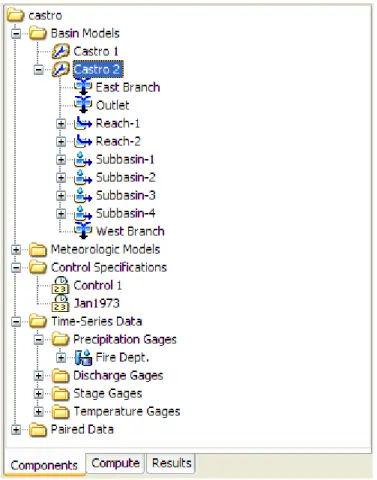
Three sample projects are included with the program. The "Castro" project shows how the program can be used for basic hydrology. The "Tenk" project demonstrates the capability of the program to use gridded precipitation. Finally, the "Tifton" project exhibits continuous simulation with the soil moisture accounting method. The

projects are kept in a space-saving, compressed form. They can be extracted for use at any time by going to the Help menu and selecting the Install Sample Projects…

(32)

(33)

C H A P T E R 3

Overview

This chapter describes the basics of working with the program. It includes

descriptions of the main parts of the interface. Specific details of when and how data are saved is also included. Conventions are provided for the formatting of input data, the use of units, and interpolation. An outline of the best way to use the program is also provided.

Program Screen

The program screen contains a title bar, menu system, toolbar, and four panes. These panes will be referred to as the Watershed Explorer, Desktop, Component Editor, and the Message Log as shown in Figure 1. The title bar displays the version of the program used and the location of the currently-open project. The other parts of the program screen are discussed in detail in this chapter.

Desktop Watershed Explorer Message Log Component Editor

Figure 1. The main program screen with Watershed Explorer in the upper left, Component Editor in the lower left, Message Log at the bottom, and Desktop using the remaining area.

(34)

Menu System

The menu system contains several menus to help you use the program. Each menu contains a list of related commands. For example, the Parameters menu contains a list of commands to open global parameter tables for viewing and editing parameters required by hydrologic elements in the selected basin model. Items in an individual menu are inactive (cannot be selected) if the command can not be carried out by the program at the current time.

Commands for managing the opened project are available from the File menu. File

menu items and the resulting actions are provided in Table 1. The last four projects opened are shown at the bottom of the File menu. Click on one of the project names to open the project.

The Edit menu contains commands for editing hydrologic elements in the selected basin model. If no basin model is selected, then all commands in this menu are inactive. Edit menu commands and the resulting actions are provided in Table 2. Additional Edit menu includes commands select mouse tools for use in the Basin Model Map.

The View menu contains a list of commands for working in the basin map. These commands are inactive if no basin model is open in the Desktop. A list of View menu items and the resulting actions are provided in Table 3.

Table 1. Commands available from the File menu.

File Menu Commands Action

New… Create a new project.

Open… Open a project.

Import ⇒ Import HEC-1 files, basin or meteorologic models, and control specifications

Save Save the current project.

Save As… Make a copy of the current project.

Delete Delete the current project.

Rename Rename the current project.

Backup… Create a backup copy of the current project, or restore to the last backup that was made.

Print… Print the currently selected item.

Exit Exit the program.

Table 2. Commands available from the Edit menu.

Edit Menu Commands Action

Cut Cut or delete the selected hydrologic element(s).

Copy Make a copy of the selected hydrologic element(s).

Paste Paste the copied hydrologic element(s).

Select All Select all hydrologic elements in the basin model.

Clear Selection Unselect all selected hydrologic elements in the basin model.

(35)

Table 3. Commands available from the View menu.

View Menu Commands Action

Maximum Extents Open the maximum extents editor.

Background Maps Open the map layer selector editor.

Draw Gridlines Toggle showing gridlines in the basin map.

Zoom In Zoom in by a factor of 25%.

Zoom Out Zoom out by a factor of 50%.

Zoom To Selected Zoom to the current element selection.

Zoom To Maximum Extents Zoom out to the maximum extents.

Draw Element Icons Toggle showing of element icons .

Draw Map Objects Toggle showing of element polygons and polylines.

Draw Element Labels Toggle showing of labels in different formats .

Draw Flow Directions Toggle flow direction arrows on reach elements.

Rescale Elements Scale the locations of the selected elements.

Lock Element Locations Toggle allowing element locations to be changed.

Lock Hydrologic Order Toggle allowing sorting and reordering.

Clear Messages Clear all messages from the message window.

Table 4. Commands available from the Components menu.

Components Menu Commands Action

Basin Model Manager Open the basin model manager.

Meteorologic Model Manager Open the meteorologic model manager.

Control Specifications Manager Open the control specifications manager.

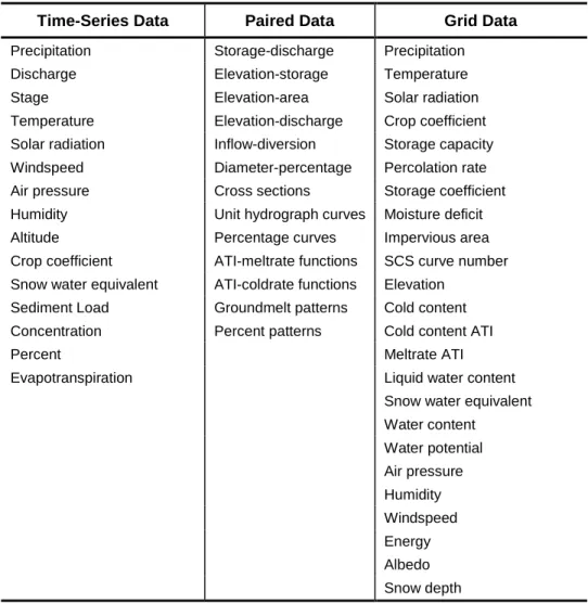
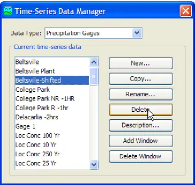
Time-Series Data Manager Open the time-series data manager.

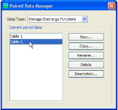
Paired Data Manager Open the paired data manager.

Grid Data Manager Open the grid data manager.

Component managers are opened from the Components menu. Program

components include basin models, meteorologic models, control specifications, time-series data, paired data, and gridded data. A list of Components menu items and the resulting actions are provided in Table 4.

The Parameters menu contains menu commands to open global parameter editors. Global parameter editors let you view and edit subbasin and reach parameters for elements using the same methods (subbasin canopy, surface, loss, transform, and baseflow methods and reach routing and gain/loss methods). Global parameter menu options are only active if subbasin or reach elements in the basin model use the method. For example, if the Parameter ⇒ Loss menu option is selected, a submenu with all loss methods opens. Only loss methods used by subbasin elements in the current basin model will be active in the menu. If hydrologic elements are selected in the basin model, then the selected elements determine what menu items are

available. The Parameters menu also contains menu commands to change subbasin canopy, surface, loss, transform, and baseflow methods and reach routing and gain/loss methods. If subbasin or reach elements are selected in the basin model, then only the selected elements will change methods. The last menu