The Securitization of Longevity Risk and its Implications for Retirement Security

ScholarlyCommons

ScholarlyCommons

Wharton Pension Research Council Working

Papers Wharton Pension Research Council

10-1-2013

The Securitization of Longevity Risk and its Implications for

The Securitization of Longevity Risk and its Implications for

Retirement Security

Retirement Security

Richard D. MacMinn

Illinois State University, [email protected] Patrick Brockett

University of Texas at Austin, [email protected] Jennifer Wang

National Cheng-Chi University, [email protected] Yijia Lin

University of Nebraska Lincoln, [email protected] Ruilin Tian

North Dakota State University, [email protected]

Follow this and additional works at: https://repository.upenn.edu/prc_papers Part of the Economics Commons

MacMinn, Richard D.; Brockett, Patrick; Wang, Jennifer; Lin, Yijia; and Tian, Ruilin, "The Securitization of Longevity Risk and its Implications for Retirement Security" (2013). Wharton Pension Research Council Working Papers. 128.

https://repository.upenn.edu/prc_papers/128

The published version of this Working Paper may be found in the 2014 publication: Recreating Sustainable Retirement: Resilience, Solvency, and Tail Risk.

This paper is posted at ScholarlyCommons. https://repository.upenn.edu/prc_papers/128 For more information, please contact [email protected].

Abstract Abstract

The economic significance of longevity risk for governments, corporations, and individuals has begun to be recognized and quantified. The traditional insurance route for managing this risk has serious

limitations due to capacity constraints that are becoming more and more binding. If the 2010 U.S.

population lived three years longer than expected then the government would have to set aside 50% of the U.S. 2010 GDP or approximately $7.37 trillion to fully fund that increased social security liability. This is just one way of gauging the size of the risk. Due to the much larger capacity of capital markets more attention is being devoted to transforming longevity risk from its pure risk form to a speculative risk form so that it can be traded in the capital markets. This transformation has implications for governments, corporations and individuals that will be explored here. The analysis will view the management of

longevity risk by considering how defined contribution plans can be managed to increase the sustainable length of retirement and by considering how defined benefit plans can be managed to reduce pension risk using longevity risk hedging schemes.

Keywords Keywords

Longevity Risk, Retirement, Securitization, Buy-Out, Longevity Swap Disciplines

Disciplines Economics Comments Comments

The published version of this Working Paper may be found in the 2014 publication: Recreating Sustainable Retirement: Resilience, Solvency, and Tail Risk.

1

Recreating Sustainable

Retirement

Resilience, Solvency, and Tail Risk

EDITED BY

Olivia S. Mitchell,

Raimond Maurer, and

P. Brett Hammond

Great Clarendon Street, Oxford, OX2 6DP, United Kingdom

Oxford University Press is a department of the University of Oxford. It furthers the University’s objective of excellence in research, scholarship, and education by publishing worldwide. Oxford is a registered trade mark of Oxford University Press in the UK and in certain other countries

© Pension Research Council, The Wharton School, University of Pennsylvania 2014 The moral rights of the authors have been asserted

First Edition published in 2014 Impression: 1

All rights reserved. No part of this publication may be reproduced, stored in a retrieval system, or transmitted, in any form or by any means, without the prior permission in writing of Oxford University Press, or as expressly permitted by law, by licence or under terms agreed with the appropriate reprographics rights organization. Enquiries concerning reproduction outside the scope of the above should be sent to the Rights Department, Oxford University Press, at the address above

You must not circulate this work in any other form and you must impose this same condition on any acquirer

Published in the United States of America by Oxford University Press 198 Madison Avenue, New York, NY 10016, United States of America British Library Cataloguing in Publication Data

Data available

Library of Congress Control Number: 2014940448 ISBN 978–0–19–871924–3

Printed and bound by

CPI Group (UK) Ltd, Croydon, CR0 4YY

Links to third party websites are provided by Oxford in good faith and for information only. Oxford disclaims any responsibility for the materials contained in any third party website referenced in this work.

List of Figures ix

List of Tables xiii

Notes on Contributors xv

1. Recreating Retirement Sustainability 1

Olivia S. Mitchell and Raimond Maurer

Part I. Capital Market and Model Risk

2. Managing Capital Market Risk for Retirement 9

Enrico Biffis and Robert Kosowski

3. Implications for Long-term Investors of the Shifting Distribution of

Capital Market Returns 30

James Moore and Niels Pedersen

4. Stress Testing Monte Carlo Assumptions 60

Marlena I. Lee

Part II. Longevity Risk

5. Modeling and Management of Longevity Risk 71

Andrew Cairns

6. Longevity Risk Management, Corporate Finance, and Sustainable

Pensions 89

Guy Coughlan

7. Model Risk, Mortality Heterogeneity, and Implications for Solvency

and Tail Risk 113

Michael Sherris and Qiming Zhou

8. The Securitization of Longevity Risk and Its Implications for

Retirement Security 134

Part III. Regulatory and Political Risk

9. Evolving Roles for Pension Regulations: Toward Better Risk Control? 163

E. Philip Davis

10. Developments in European Pension Regulation: Risks and Challenges 186

Stefan Lundbergh, Ruben Laros, and Laura Rebel

11. Extreme Risks and the Retirement Anomaly 215

Tim Hodgson

Part IV. Implications for Plan Sponsors

12. Risk Budgeting and Longevity Insurance: Strategies for Sustainable

Defined Benefit Pension Funds 247

Amy Kessler

13. The Funding Debate: Optimizing Pension Risk within a Corporate

Risk Budget 273

Geoff Bauer, Gordon Fletcher, Julien Halfon, and Stacy Scapino

The Pension Research Council 293

The Securitization of Longevity Risk and Its

Implications for Retirement Security

Richard MacMinn, Patrick Brockett, Jennifer Wang, Yijia Lin, and

Ruilin Tian

The simplest notion of individual longevity risk is that it is the possibility that one will outlive one’s accumulated wealth. The risk of outliving one’s accumulated wealth has many unpleasant consequences for individuals and societies, and because the risk is increasing it must be addressed. If an individual is covered by a defined con-tribution (DC) plan, the employee contributes to the plan until retirement. The employer may or may not match the employee’s contribution. Accumulated wealth generated during the individual’s working life yields the wealth that the individual will use to generate a retirement income stream. If the individual is covered by a defined benefit (DB) plan, the employer guarantees to provide the employee a designated amount of money upon retirement up until the employee’s death. The employee may or may not contribute to the plan. The designated amount is based on the employee’s earnings, length of employment, and age. With a DC plan, the employee is responsible for ensuring that enough money has been contributed to the account to avoid longevity risk. With a DB plan, the employer is liable for ensur-ing that the plan does not run out of money before the employee dies. In the first case the individual faces the longevity risk, while in the second case the pension provider faces the longevity risk.

Both plans have distinctive risks and in this chapter we examine the risks from the perspective of the individual and the institution. Longevity risk is important in part because of its size; international pension liabilities have been estimated at approxi-mately $21 trillion. Longevity risk is also important because as life expectancy increases, individuals must increase contributions to their DC plans to mitigate lon-gevity risk and the size of the necessary additional contribution is uncertain, as it depends in part on how life expectancies change over time. Hence the questions of interest here include: What happens to the financial well-being of a retired cohort in the event of an unexpected change in life expectancy or financial stability? What happens if it does not manage these risks? What happens if it does manage these risks using currently available instruments? How might it manage the longevity risk with longevity instruments?

In what follows, we first explore the meaning of longevity risk and consider its magnitude. Next we consider how mortality and longevity risks have been

transformed from pure risks to speculative risks. Subsequently we examine longev-ity risk and financial market risks from the perspective of those who bear them; we show a need for more longevity instruments in the retail market and some of the benefits of the existing longevity instruments in the wholesale market for longevity risk. A final section concludes.

Longevity Risk

Risk can be defined as the negative consequences of uncertainty. Both uncertainty (multiple possible outcomes) and negative consequences are necessary prerequi-sites for risk to exist (Baranoff et al. 2009). Since most people find longer life desir-able, the term ‘longevity risk’ needs further explication to provide the context in which longevity presents a ‘risk’ rather than a ‘benefit’ to individuals and/or insti-tutions. Longevity risk is the risk that an individual life span or the average popula-tion life span will exceed expectapopula-tions. The negative consequences of an extended life span can include outliving one’s friends, diminished mobility and cognitive flexibility/focus, and outliving one’s financial resources after retirement without the remedial possibility of rejoining the workforce to produce necessary income at the later date wherein the probability (or the eventuality) that financial assets will soon be depleted becomes recognized. Longevity risk has an unsystematic or idiosyncratic component, as well as a systematic component. The idiosyncratic component is sometimes described as the risk of an individual outliving one’s accu-mulated wealth; Milevsky (2006) describes this as ‘retirement ruin.’ The systematic component corresponds to the more general hazard that people in the aggregate will live longer than expected (Oppers et al. 2012), thus causing strain on pensions, employers, and society in general. The systematic component is often referred to as aggregate longevity risk in the literature (MacMinn et al. 2006; Blake et al. 2013). The aggregate longevity risk discussed here is the risk of living longer than one expects; it is also a systematic risk because life expectations are themselves random variables.

From a financial perspective, the unsystematic component of longevity risk may be handled by holding a sufficiently diversified and adequately funded asset portfolio to decumulate during retirement. If life expectancy were certain, the individual could purchase an annuity certain designed to provide the desired cash flow for the certain life expectancy. Alternatively, the individual could pur-chase a bond with the desired flow of coupon payments and leave the principal repayment as a bequest to beneficiaries but because life expectancy is uncertain, the individual must design a portfolio of assets to provide a desired cash flow for an undetermined period of time. This portfolio may consist of equity, bonds, and possibly a life annuity. The life annuity is an asset that provides a specified cash flow for the remaining years of an individual’s life. If the unsystematic component of life expectancy were the only risk faced by an individual then

a life annuity may be shown to dominate other assets (Yaari 1965). However, the risk of outliving one’s accumulated wealth is not the only unsystematic risk. Increased life expectancy includes morbidity (and other) risks as well, implying that just a life annuity would not cover a long-term illness, dementia, etc., and therefore a diversified asset portfolio is still needed (Sinclair and Smetters 2004; Horneff et al. 2009; MacMinn and Weber 2010; Chai et al. 2011).

From a financial perspective, at the firm or society level, aggregate longevity risk (the systematic component) must be managed. The management choices include bearing the risk or transferring or trading the risk to some other entity willing to bear it. In deciding among these alternatives, a determination must be made on how to price this risk transfer appropriately. This aspect of longevity risk might be thought of as a trend risk or the risk of underestimating life expectancy (Blake et al. 2013). Alternatively, as noted, we may think of life expectancy itself as a random variable. Oeppen and Vaupel (2002) show the record life expectancy for females as projected by a number of authors and organizations and report the rather sur-prising result that the record female life expectancy has increased by three months per year for more than 150 years. Hence, Oeppen and Vaupel also show that each historical life expectancy prediction has been wrong. With reference to 2005 mor-tality rates, they note that U.K.  mormor-tality rates had declined over the previous

10–15 years by over 2 percent per annum for the age groups over 60. Referring to

the 2 percent decline and using government actuarial department (GAD) figures, Turner made the following comment about mortality rates (2006: 562):

If they continue at that rate, male life expectancy at sixty-five, currently esti-mated at nineteen, will reach about thirty by 2050. If the rate accelerates to 3 percent, life expectancy would soar to 37 years. Only if it decelerates to 1 percent would the GAD’s 2002-based principal projection of 22 years in 2050 be correct. So the GAD 2002 projection—a major increase from previ-ous projections—nevertheless still assumed a major deceleration of mortality rate improvement.

The errors in life expectancy estimates noted here highlight the systematic risk of longevity risk and the magnitude of the risk.

It is important to understand the vast financial size of the longevity risk problem. Turner (2006) estimated £2.5 ($4.3) trillion in liabilities subject to longevity risk in the U.K. Swiss Re has since estimated $20.7 trillion in pension liabilities subject to longevity risk internationally (Burne 2011). Oppers et al. (2012: 8) provide a different perspective by calculating the cost of maintaining the retirement living standard due to aging and longevity shocks as a percentage of gross domestic prod-uct (GDP) for advanced and emerging countries. Using the demographic trends predicted by the United Nations, they note:

In the baseline population forecast and with a 60 percent replacement rate, the annual cost rises from 5.3 percent to 11.1 percent of GDP in advanced

economies and from 2.3 percent to 5.9 percent of GDP in emerging econo-mies . . . Taken over the full period, the cumulative cost of this increase because of aging in this scenario is about 100 percent of 2010 GDP for the advanced economies and about half that amount in emerging economies.

The authors also observe that a longevity shock of three years would add almost an additional 50 percent to these cumulative costs of aging by 2050. There is uncertainty surrounding all of these predictions, but the magnitudes are hard to ignore.

Ignoring longevity risk is indeed a significant problem. Oppers et al. (2012) use data from the U.S. Department of Labor (DOL) to estimate the longevity risk faced by DB plans. They report many plans used outdated mortality tables; the majority of the plans used the 1983 Group Annuity Mortality (GAM) until recently. Using out-of-date mortality tables exposes pension plans to longevity risk and risk of ruin. Dushi et al. (2010) compare pension liability values based on the plans’ longevity assumptions versus the pension liability values forecast by the Lee–Carter mortal-ity model and find that the outdated mortalmortal-ity tables could understate the pension liability for a typical male participant by approximately 12 percent.

Longevity risk can be borne or transferred, in whole or in part. The retail market for longevity risk allows consumers to transfer all or part of the risk with life annui-ties. In the U.K., this market amounts to £135 billion, but this is because consumers

are required by law to at least annuitize before they turn 75 (Loeys et al. 2007).1 _The

retail or life annuity market remains very small in the U.S. since there is no similar requirement that individuals annuitize when they retire. In fact, this general lack of a sizable life annuity market has been described as the annuity puzzle, since Yaari (1965) and Davidoff et al. (2005), among others, have shown that in the absence of a bequest motive, the life annuity instrument for retirement funding dominates other asset choices.

A wholesale market for longevity risk would allow pension funds and insurers the ability to transfer some of the longevity risk rather than bearing it. The U.K. whole-sale market has been active and many of the transactions take the form of buyouts

and buy-ins.2 _{In a buyout, there is a transfer of pension assets and liabilities for a}

particular cohort; the cost of the buyout is the difference between the values of the assets and the liabilities transferred. The difference between the asset and liability values may be covered by a loan with a known cash flow that is well understood by investors. In the buy-in, there is a bulk purchase of annuities from an insurer to hedge the risk of the liabilities associated with one or more cohorts. This immu-nizes the pension fund from the liability risk for the cohorts covered.

The retail and wholesale markets noted here do provide a transfer mechanism for the market participants but the mechanisms are crude instruments. More than one risk is transferred and the risks are aggregated rather than disaggregated; this generates more concentration of risk and hence amplifies the eventual probability of insolvency for those concentrations. Given the size of the longevity risks, this

becomes a new problem that is inconsistent with the history of financial markets. ‘Indeed, the history of the development of risk instruments is a tale of the progres-sive separation of risks, enabling each to be borne in the least expenprogres-sive way’ (Kohn 1999: 2).

Securitization

Longevity risk has put corporations, governments, and individuals under a sig-nificant financial burden. One common way to manage this risk is securitization (i.e. isolating the cash flows that are linked to longevity risk and repackaging them into cash flows that are traded in capital markets). The earliest securitizations were ‘block of business’ securitizations used to capitalize expected future profits from a

block of life business, such as to recover embedded values3 _{or to exit from a}

geo-graphical line of business. Cowley and Cummins (2005) introduced the early devel-opment of the securitization in life insurance. More recently, Blake et al. (2013) provided a more comprehensive and global overview of the emergence of the mar-ket in traded assets and liabilities linked to longevity and mortality and referred to this market as the New Life Market. They noted that the New Life Market would act as a catalyst to help facilitate the development of annuity markets both in the developed and the developing world and protect the long-term global viability of retirement income provision.

The idea of mortality securitization was initially proposed by Cox et al. (2000). The first mortality bond, known as Vita I, was issued by Swiss Re in 2003; it was designed to hedge mortality risk rather than to hedge longevity risk. Nevertheless, it provides an important successful example of a Life Market instrument. Vita I  was a success, and led to additional bonds being issued to investors on less

favorable terms.4 _{Blake and Burrows (2001) were the first to advocate the use of}

mortality-linked securities to transfer longevity risk to capital markets. They sug-gested that the governments should help pension funds and insurance compa-nies hedge their mortality risks by issuing survivor bonds. In 2004, the European Investment Bank (EIB) and BNP Paribas launched a longevity bond that was the first securitization instrument designed to transfer longevity risk; ultimately it was not issued due to insufficient demand. Design issues, such as the introduction of basis risk, pricing issues, institutional issues, and educational issues, were among the reasons why the EIB/BNP bond did not launch (Lin and Cox 2008).

The lack of success in issuing long-dated longevity bonds has led to a derivatives design effort. Various new securitization instruments and derivatives for longev-ity risk, such as mortallongev-ity forwards, survivor swaps, survivor futures, and survivor

options have received attention among academics and practitioners.5 _{In 2007, J.P.}

Morgan introduced the first capital market derivative for a longevity hedge; it has

become known as a ‘q-forward.’ A q-forward can be used to hedge the value of the

pension liability or the associated cash flows. More complex, life-related derivatives

of q-forwards can be used to replicate and to hedge the longevity exposure of an annuity or a pension liability or to hedge the mortality exposure for a book of life

business. Following the introduction of a q-forward transaction, a longevity swap

was used to exchange actual pension payments for a series of pre-agreed fixed payments. This particular swap was legally constituted as an insurance contract and was not a capital market instrument. There have been 16 publicly announced transactions of longevity swaps executed between 2007 and 2012 in the U.K. (Blake et al. 2013).

A Financial Market Model

Suppose the financial market consists of the S&P 500 index, the Merrill Lynch corporate bond index, and a three-month T-bill. Following Cox et al. (2013), we

describe the return dynamics of the S&P 500 index as A_1,t and the Merrill Lynch

corporate bond index as A_2,t at time t as a combination of Brownian motion and

a compound Poisson process. The stochastic process of the three-month T-bill

return A_3,t is simply described as Brownian motion. The three returns are as follows:

At t At k Wt Yj j N N t t A 1 1 1 12 1 1 1 1 1 1 2 1 ,+ ∆| ,exp ( ) > =  − − ∆ + ∆    + F α σ λ σ 11

∏

(8.1) At t At k Wt Y j j N N t t A 2 2 2 22 2 2 2 2 2 1 2 2 ,+∆| , exp ( ) > =  − − ∆ + ∆    + F α σ λ σ 22

∏

(8.2) A3t t A3t 3 32 3 W3t 1 2 ,+∆| = , exp ( − )∆ + ∆    F α σ σ (8.3)

where the constants α α α1, ,2 3 and σ σ σ1, ,2 3 are the drift and volatility

meas-ures of the S&P 500 return, the Merrill Lynch corporate bond return, and the

three-month T-bill rate given no jumps. The parameter k1≡E Y( 1−1) is the

expected percentage change in the S&P 500 return and k₂ is similarly defined for

the Merrill Lynch corporate bond return if a Poisson event occurs. The parameters

λ1 and λ2 are the mean numbers of arrivals per unit time of the Poisson processes

Nt1 and Nt2 respectively. The jump size Y1j or Y2j is independent and identically

distributed as a lognormal random variable with the size parameter m₁ and the

volatility parameter S₁ or m₂ and S₂. _Y1j andY2j are independent for all i and j. The

correlation between the standard Brownian motions of the S&P 500 index and the

Merrill Lynch corporate bond index, W_1t and W_2t, is captured by the correlation

coefficient ρ12 (i.e.Cov W W( 1t, 2t)=ρ σ σ12 1 2t).

We further assume the three-month T-bill is uncorrelated with either the S&P 500 index or the Merrill Lynch corporate bond index. Based on the annual data of the S&P 500 and the Merrill Lynch corporate bond provided by the DataStream

and the three-month T-bill rates from FRED at Federal Reserve Bank of St. Louis from 1989 to 2010, we estimate models (8-1), (8-2), and (8-3) to obtain the model parameters. The estimated parameters are based on annual data and are reported in Table 8.1.

In what follows we will use these estimates to forecast returns for investor portfo-lios and for DB plans.

DC Plans

Given the financial market model developed in the previous section, suppose the

individual investor or, equivalently, the retiree selects a portfolio ( ,ω ω ω1 2, 3) in the

S&P 500 index, the Merrill Lynch corporate bond index, and the three-month T-bill, respectively. Given our interest in longevity risk we investigate the length of a sustainable retirement period under the following two assumptions: (1) The

indi-vidual invests in a TIAA-CREF-type lifecycle fund;6 _{(2) The individual invests in a}

portfolio based on his own preferences.

Assumption (1): Investment in a TIAA-CREF-type Lifecycle Fund

The TIAA-CREF Lifecycle Funds consist of a series of target retirement date funds in five-year increments (2010, 2015, 2020, etc.), where an investor selects the fund that most closely matches his or her retirement year (e.g. a Lifecycle 2040

Table 8.1 Maximum likelihood parameter estimates of three pension assets using annual data

Parameter Estimate Parameter Estimate Parameter Estimate

α1 0.0866 α2 0.0691 α3 0.0515

σ1 0.0864 σ2 0.0547 σ3 0.0329

λ1 0.2742 λ2 0.0505 ρ12 0.6016

m1 −0.3048 m2 −0.1468

s1 0.0000 s2 0.0000

Notes: α1,α2,α3 and σ1,σ2,σ3are the drift and volatility measures of the returns of the S&P

500 index, Merrill Lynch corporate bond index, and three-month T-bill. λ1 and λ2 are the mean

numbers of arrivals per unit time of the Poisson processes for the returns of the S&P 500 and Merrill Lynch corporate bond indices. m₁(m₂) and _s1(_s2) are the size parameter and volatility parameter of the lognormal jump size for the return of S&P 500 (Merrill Lynch corporate bond) index. ρ12is the correlation coefficient between the geometric Brownian motions of the returns of S&P 500 and Merrill Lynch corporate bond indices.

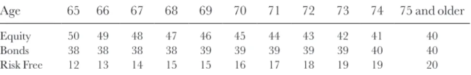
Fund is for an investor planning to retire in or around 2040). The funds are profes-sionally managed and automatically adjust over time. For a retiree who invests in a TIAA-CREF-type Retirement Fund, the portfolio allocation at different ages is

illustrated in Table 8.2.7

Assumption (2): Investment in a Self-selected Portfolio.

To consider all possible combinations ofω1and ω2, we note that short selling is

not allowed. In this case the investment in equity and bond indices satisfies

0≤ω ω₁+ ₂≤1.

Investor Portfolio Analysis

We investigate the sustainable length of a retiree’s retirement savings when the financial market experiences the following two scenarios:

Base Case

Suppose the financial market maintains the same trend and volatility that it has

demonstrated over the past 20 years.8 _{As such, we use the parameters in Table 8.1}

calibrated with historical data to forecast the returns of the three pension assets. Under the Base case, the stock market will experience about 10/(1/0.2742) = 2.74 crashes every ten years. The crashes in the bond market take place less fre-quently. Every ten years, an investment in corporate bonds is expected to face 10/

(1/0.505) = 0.51 crashes.9

BaseX2 Case

Suppose financial crashes happen twice as frequently as what the market

experi-enced in the past 20 years. As such, we double the parameters λ1, m1, and s1 for the

stock index and λ2, m2, and s2 for the bond index. Under the BaseX2 case, the stock

and bond markets will experience 5.48 and 1.01 crashes every ten years.

Table 8.2 Asset allocation at different ages (percentage)

Age 65 66 67 68 69 70 71 72 73 74 75 and older

Equity 50 49 48 47 46 45 44 43 42 41 40

Bonds 38 38 38 38 39 39 39 39 39 40 40

Risk Free 12 13 14 15 15 16 17 18 19 19 20

Note: All the numbers for equity, bonds, and risk-free assets are in percentages.

We simulate the returns of three pension assets from t = 0 when the individual retires. Based on the United States male population mortality data from 1901 to

2007,10 _{we assume the maximal age he can live is 103. For each yield path, we}

simu-late 58 years after t = 0. Suppose the initial retirement fund at time 0 is M₀ = M and

the retiree withdraws W_d per period starting from t = 1. The value of the retirement

fund M_t at time t depends on the amount invested in asset i at time t−1, A_i,t−1 and its

return in period t and r_i,t. Hence,

Mt Ai t r t i i t = − + = =

∑

, 1( ,), , , ,... 1 3 1 1 2 3 (8.4)

and the following equation holds for the retiree:

Ai t M W t i t d , , , , ,... =

∑

= − = 1 3 1 2 3 (8.5)

The sustainable length of the retirement fund, S, is calculated as:

S=max

{

t N∈ +|Mt ≥Wd

}

(8.6)

We run 1,000 simulations with the market parameters to generate 1,000 yield

paths for each pension asset. For each yield path, we calculate sustainable length Si

based on equations (8.4), (8.5), and (8.6). For the random variable S , we

investi-gate three measures (the mean, VaR_1%, and CVaR_1%) as shown in models (8.7), (8.8),

and (8.9) respectively. E S E Si i ( ) =     =

∑

1 1000 (8.7) VaR S1%( ) = =s min

{

s R∈ |P

{ }

S s≥ ≤99%

}

(8.8) CVaR S1%( ) =E S S s

{

| ≤

}

(8.9)

whereSstands for the sustainable length of the retiree’s retirement fund, VaR S1%( )

gives the smallest sustainable period such that the probability of observing a

sus-tainable period greater than it is 99 percent, and CVaR S1%( ) gives the expected

sus-tainable period conditional on the sussus-tainable period being shorter than VaR S1%( ) .

The impact of portfolio allocation on the mean, VaR_1%, and CVaR_1% of the

sustain-able length is sensitive to the initial retirement savings M and the annual withdrawal

W_d, which can be explained following two lines of thought that lead to opposite

a negative relationship between the mean and CVaR_1% (or VaR_1%) because the latter is a measure of risk. Second, the mean and the tail expectation of a random vari-able could move in the same direction, since both come from the same distribution.

Results for the TIAA-CREF-type Lifecycle Fund

Given an initial retirement fund M = $1,000,000, we assume the retiree invests in

a TIAA-CREF-type retirement fund. That is, the portfolio allocation changes over time as specified in Table 8.2. The sustainable length of the fund for the Base case and the BaseX2 case under different annual withdrawal strategies is illustrated in Table 8.3.

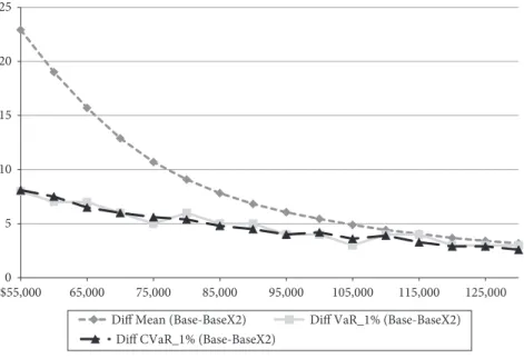
We further investigate how the individual’s funding status would be affected if the financial market deteriorates due to more frequent crashes (BaseX2 case). Setting the Base case as the benchmark, the influence of market deterioration on the individual retirement fund is expressed as the difference of the sustainable

length between the Base and BaseX2 cases. The differences in mean, VaR1%, and

CVaR1% are illustrated in Figure 8.1. Figure 8.1 shows that if the financial markets

0 5 10 15 20 25 $55,000 65,000 75,000 85,000 95,000 105,000 115,000 125,000 Diff Mean (Base-BaseX2) Diff VaR_1% (Base-BaseX2)

Diff CVaR_1% (Base-BaseX2)

Figure  8.1. Comparison between Base and BaseX2 cases for an investor holding a TIAA-CREF-type retirement fund.

Note: The Base case assumes the financial market maintains the same trend and volatility that it has demonstrated throughout the past 20 years. The BaseX2 case supposes financial crashes happen twice as frequently as the market has experienced in the past 20 years. The vertical axis shows the sustainable periods in years and the horizontal axis is the annual withdrawal.

T able  8.3 Sustainab le lengths w hen in vesting in a TIAA-CREF-type retir ement fund Base Case BaseX2 Case W ithdra w ($) Mean ($) Va R1% ($) CV aR1% ($) W ithdra w ($) Mean ($) Va R1% ($) CV aR1% 55,000 35.305 14 13.4971 55,000 12.382 6 5.3951 60,000 30.558 13 12.5974 60,000 11.541 5.99 5.09 65,000 26.501 12 11.4963 65,000 10.795 5 4.9999 70,000 23.054 11 10.5974 70,000 10.163 5 4.5975 75,000 20.281 10 9.8996 75,000 9.574 5 4.2936 80,000 18.154 10 9.395 80,000 9.068 4 4 85,000 16.411 9 8.799 85,000 8.588 4 4 90,000 15.016 9 8.4963 90,000 8.19 4 4 95,000 13.862 8 7.8996 95,000 7.801 4 3.8996 100,000 12.877 8 7.5974 100,000 7.433 4 3.3951 105,000 12.024 7 6.8996 105,000 7.131 4 3.2936 110,000 11.267 7 6.8996 110,000 6.846 3 3 115,000 10.612 7 6.2935 115,000 6.542 3 3 120,000 10.008 6 5.8996 120,000 6.323 3 3 125,000 9.483 6 5.8996 125,000 6.07 3 3 130,000 9.023 6 5.5975 130,000 5.837 3 3 Notes : T he Base case assumes the financial mar ket maintains the same tr end and vola tility tha t it has demonstra ted thr oughout the past 20  year BaseX2 case supposes financial crashes happen twice as fr equently as w ha t the mar ket experienced in the past 20  year s. Sour ce : A uthor s’ calcula tions; see te xt.

become more volatile, in the sense that crashes become more frequent, then the individual can expect to lose more than 20 periods from the sustainable retirement fund. Figure 8.1 and Table 8.3 also show that, under the same circumstances, a

retiree can lose eight sustainable periods from the VaR1% at the lowest annual

with-drawal ($55,000). Finally, the difference in CVaR represents the loss in sustainable periods in the tail of the distribution sustainable periods and Figure 8.1 shows that for the lowest withdrawal rate the investor can expect to lose 8.1 of the sustainable retirement periods; the expected tail loss eventually diminishes with the withdrawal rate since the number of sustainable retirement periods also diminishes.

When both the initial fund M and annual withdrawal W_d are allowed to change,

we demonstrate the impact of M and W_d on the sustainable number of periods in

Figure 8.2. This figure shows that the BaseX2 case deteriorates from the Base case. As one expects, the figure shows that the sustainable number of retirement years

increases with M and decreases with W_d. Given M = $1,000,000 and W_d = $55,000,

the expected number of sustainable retirement periods is 35 in the Base case, while

it is about 13 periods if W_d is increased to $100,000.

If the investor realizes returns in the tail of the portfolio distribution, then the

CVaR1%1 yields 13 and 8 periods for these two withdrawal rates respectively in the

Base case. Again given M = $1,000,000, the expected number of sustainable

retire-ment periods is greater than the life expectancy of a 65-year-old U.S. male (i.e. 19.4 years) if he withdraws no more than $75,000 per year; even here, however, a withdrawal rate of $55,000 will not sustain that 65-year-old to his life expectancy.

Since there is a 30 percent chance that the 65-year-old will live to 90, the M =

$1,000,000 and W_d = $55,000 may be adequate unless he experiences returns in

the tail of the portfolio distribution; then the sustainable retirement period is clearly inadequate. In the event that crashes are more frequent, Table 8.3 shows that given

M = $1,000,000 and W_d= $55,000, the expected and conditional tail-expected

val-ues for sustainable periods become 12.38 and 5.4 respectively. Hence, the expecta-tions fall far short of the life expectancy if the financial market deteriorates, as in the BaseX2 case. One of the additional difficulties for the investor facing financial risk and longevity risk is that his perceived life expectancy may fall short of his actual life expectancy (i.e. the individual may get the trend wrong).

Results for Other Portfolios

Next we suppose the investor selects a portfolio for retirement based on his own

preferences.11 _{Given an initial retirement asset M at t = 0 of $1,000,000, we show}

how the sustainable periods are affected by the annual withdrawal Wd and

port-folio allocation under the Base and BaseX2 scenarios. Figures 8.3 and 8.4 show

the mean and CVaR1% of the sustainable lengths respectively. The three surfaces

from top to bottom stand for sustainable periods with withdrawal rates of $75,000, $100,000, and $125,000 respectively. As Figure 8.3 shows, in the Base case, the

4 6 8 10 12 14 0.5 1 1.5 0 10 20 30 40 50 Withdraw

Mean of Support Length TIAA-CREF

Total Funds Base BaseX2 5 6 7 8 9 10 11 12 0.5 1 1.5 0 5 10 15 20 Withdraw Total Funds Base BaseX2 × 10 6 × 10 6 × 10 4 × 10 CVaR 1%

of Support Length TIAA-CRE

F Figure  8.2 . Mean and CV aR1% of sustainab le lengths giv en differ ent initial sa

vings and ann

ual withdra wals f TIAA-CREF-type lifecy cle portf olio . Note : T he Base case assumes the financial mar ket maintains the same tr end and vola tility tha t it has demonstra ted thr oughout past 20  year s. T he BaseX2 case supposed financial crashes happen twice as fr equently as the mar ket has experienced in the past 20  year s. Sour ce : A uthor s’ calcula tions; see te xt.

0 0.2 0.4 0.6 0.8 1 0 0.5 1 0 5 10 15 20 25 30 35

Mean of BaseCase (M=$1,000,000) - NoShortSel

l w1 w1 w2 w2 WD=75,000 WD=100,000 WD=125,000 0 0.2 0.4 0.6 0.8 1 0 0.5 0 5 10 15 20 25

Mean of BaseX2 Case (M=$1,000,000) - NoShortSell

WD=75,000 WD=100,000 WD=125,000 Figure  8.3 . Mean of sustainab le length w hen in vesting in customiz ed portf olios . Note : T he Base case assumes the financial mar ket maintains the same tr end and vola tility tha t it has demonstra ted thr oughout the past 20  year s. T he Base X2 case supposed financial crashes happen twice as fr equently as the mar ket has experienced in the past 20  year s. w1 and w2 stand for the pr oportions of the retir ee’ s fund in vested in equity and long-ter fix ed-income securities , r espectiv ely . Sour ce : A uthor s’ calcula tions; see te xt.

0 0. 2 0. 4 0. 6 0. 8 1 0 0. 5 1 0 5 10 15 20 CV aR1% of Ba se Ca se (M =$1, 000, 000) - No Sh or tS ell w1 w1 w2 w2 WD =75, 00 0 WD =100, 00 0 WD =125, 00 0 0 0. 2 0. 4 0. 6 0. 8 1 0 0. 5 0 5 10 15 20 CV aR1% of Ba se X2 Ca se (M =$ 1, 000, 000) - No Sh or tSe WD=75,000 WD=100,000 WD=125,000 Figure  8.4 . CV aR1% of sustainab le length w hen in vesting in customiz ed portf olios . Note : T he Base case assumes the financial mar ket maintains the same tr end and vola tility tha t it has demonstra ted thr oughout the past 20  year s. T he Base X2 case supposed financial crashes happen twice as fr equently as the mar ket has experienced in the past 20  year s. w1 and w2 stand for the pr oportions of the retir ee’ s fund in vested in equity and long-ter fix ed-income securities , r espectiv ely . Sour ce : A uthor s’ calcula tions; see te xt.

generate an expected sustainable retirement of almost 35 periods given the portfo-lio ( ,ω ω ω1 2, 3) = (0, 1, 0) (i.e. the investor plunges in the bond index fund). Figure

8.3 also shows that in the BaseX2 case, the investor can generate an expected

sus-tainable retirement of almost 24 years by investing in the portfolio ( ,ω ω ω1 2, 3)=

(0, 0, 1) (i.e. the investor plunges in T-bills). Again in the case of an initial

invest-ment of M = $1,000,000 and W_d = $75,000, Figure 8.4 shows that to maximize

the number of sustainable retirement years in the tail measured by CVaR1%, the

investor should invest 30 percent of his fund in the bond index and the remaining

70 percent in T-bills (i.e., ( ,ω ω ω1 2, 3)= (0, 0.3, 0.7)) in the Base case; this portfolio

yields almost 18 sustainable retirement periods. Figure 8.4 also shows that in the BaseX2 case, the investor should choose the portfolio with 10 percent invested in

the bond index and 90 percent invested in T-bills (i.e.( ,ω ω ω1 2, 3)= (0, 0.1, 0.9))

12

to maximize the number of sustainable retirement periods in the tail; this portfo-lio yields 11 sustainable retirement periods. In other words, to reduce tail risk, the investor should choose a more conservative portfolio and invest more in risk-free assets such as T-bills.

DB Plans

DB plans put longevity risk on the pension provider, not the individual. The DB provider is a trustee who should act in the interests of the retirement cohort; we consider one retirement cohort. Since the DB plan is exposed to financial and

lon-gevity risks, one objective is to minimize the total unfunded liability (TUL) of the

plan subject to any appropriate constraints. The TUL up to the terminal age of

the retirees is defined as the present value of the sequence of unfunded liabilities.

Hence TUL is

TUL ULt t t = +

(

)

= ∞

∑

₁ 1 ρ

where the random variable UL_t is the underfunding at time t. We suppose that T is

the retirement date of the cohort. Then for t ≤ T, the plan’s unfunded liability UL_t

equals

ULt =PBOt−

(

PA Ct+

)

, t=1 2, , , .…T (8.10)

In (8.10)PBOtis the pension benefit obligation and PAt is the date t pension asset

value. When t >T, UL_t equals

where B is the survival benefit and t T− pˆx T, is the conditional expected probability

that a plan member age x at time T survives t − T years when t > T.

Following Cox et al. (2013), who investigate capital market and longevity risks, we solve the following constrained minimization problem, or equivalently the pen-sion optimization problem:

Minimize Var subject to UL E TUL CVaR t t t 1 0 1

(

+

)

       

{

}

= = ∞

∑

_ρ α TTUL i C i i i n

(

)

= ≤ ≤ = ≥ =

∑

τ ω ω 0 1 1 0 1 , = 1,2, ,n… (8.12)

In (8.12), we require the expected TUL to equal zero. To control the

under-funding risk, we impose an _α-level conditional value-at-risk (CVaR) constraint on

the total unfunded liability (i.e. E(TUL|TUL ≥ VaR_95%) = _τ).13 _{Short selling is not}

allowed for the plan, so ωi≥0.

DB Base Case

To obtain the optimal solutions for the Base case for a DB plan given the pension optimization problem in (8.12) with the Lee and Carter (1992) mortality model and the pension asset models (8.1), (8.2), and (8.3), suppose the DB plan has members

who all join the plan at age x0 =45 (t = 0) and retire at age x=65 (T = 20). The

annual survival benefit payment after retirement is B = $10 million and the pension

fund at t = 0 is $5 million. Following Cox et al. (2013), we set the pension valuation

rate at ρ=0 08. and the life annuity discount rate at r =0 05. . In addition, the

plan will amortize the unfunded liability over m=7 years as in Panteli (2010) and

following Maurer et al. (2009), we set the penalty factors on the supplementary

contributions and withdrawals at _ψ1 = _ψ2 = 0.2. Our objective is to find the optimal

pension asset allocation and contribution strategies for the plan throughout the life of the cohort.

We set year 2007 as our base year t = 0 and run a Monte Carlo simulation with

1,000 iterations to generate forecasts for the three financial asset returns and

pen-sion liabilities _PBOt for _t=1 2, , .… The downside risk parameter is set at 60 and

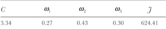
given _τ = 60, the optimal solution for (8.12) is shown in Table 8.4.

To achieve the lowest underfunding variance J and the target CVaR95%(TUL) of

60, the plan should invest 27 percent of its funds in the S&P 500 index, 43 percent in the Merrill Lynch corporate bond index, and the remaining 30 percent of its

contribution is C = 3.34. The total pension cost represents the present value of all

normal contributions, C, supplementary contributions, _SCt and withdrawals, Wt.

A higher TPC lowers the plan’s underfunding risk but imposes a higher cost on the

plan sponsor. To achieve the level of CVaR95%(TUL)= 60, the expected total

pen-sion cost is ETPC = 36.08.

Longevity Risk Effect

To examine the adverse effect of an unexpected mortality improvement on the

plan, we change the value of the Base case g in the model to other possible values;

in the Lee–Carter model, mortality is a function of a common risk factor and the

risk factor is described as a random walk with drift g. This drift g may be thought of

as the systematic risk component of mortality. A more negative value of g implies a

more substantial mortality improvement. GivenCVaR95%(TUL)=60, the adverse

effect of the longevity risk is captured by the higher E(TPC), since the plan must

adjust E(TPC) upward to reflect higher longevity risk.

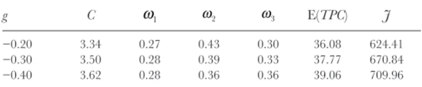
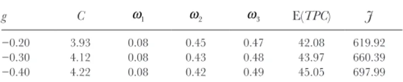
Table 8.5 shows the optimization results given different assumptions on g after

solving the optimization problem (8.12). As g decreases from the Base case −0.20

to −0.40, E(TPC) increases notably from 36.08 to 39.06 (i.e. an 8.3 percent rise);

this is due to the higher normal contribution C = 3.62 with g = −0.40, compared to

C = 3.34 with g = −0.20. The increased longevity risk increases the normal

contri-bution and puts more weight in the tails of the underfunding districontri-bution. Hence an

increase in longevity risk increases the variance J of the underfunding distribution.

That variance increases from 624.41 to 709.96 as g decreases from −0.2 to −0.4.

In addition, as g decreases, the plan invests more in the safe asset. Equivalently, the

plan manager must elect a higher portfolio weight for the safe asset, so as to satisfy

his downside risk constraint (that is, the CVaR95%(TUL) = 60).

Table 8.4 Optimal solution for the Base case with model (5.13)

C ω1 ω2 ω3 J

3.34 0.27 0.43 0.30 624.41

Notes: C stands for the normal contribution. J is the value of the objective function in Model (5-13), which measures the variance of total unfunded liability. (ω1,ω2,ω3) represents the investment

strategy where ω1,ω2, andω3are the proportions invested in the

S&P 500 index, Merrill Lynch corporate bond index, and 3-month T-bill, respectively. The Base case assumes the financial market maintains the same trend and volatility that it has demonstrated throughout the past 20 years.

Capital Market Risk Effects

To examine the capital market risk effect on the pension plan, we double the val-ues of the volatility, jump size, and jump arrival rate parameters for the S&P 500 index and the Merrill Lynch corporate bond index in Table 8.1, simulate, and resolve the optimization model (8.12). The results with the doubled parameter val-ues of the S&P 500 index and the Merrill Lynch corporate bond index are shown in Table 8.6; they provide important insights for the pension plan with respect to

possible market crashes. Given g equal to the Base case level of −0.20 and a more

volatile capital market, the E(TPC) increases by 16.6 percent from 36.08 in Table

8.5 to 42.08 in Table 8.6. In addition, to meet the downside risk constraint, the

annual normal contribution C increases by 17.8 percent to 3.93 and the proportion

invested in the low-risk three-month T-bill rises by 54 percent to ω3 = 0.47,

com-pared with the Base case levels of C = 3.34 and ω3 = 0.30 in Table 8.5.

It is worth noting that if the adverse longevity and capital market events both

occur, it will push up the expected total pension cost E(TPC) dramatically by

24.9 percent, from 36.08 in Table 8.5 to 45.05 in Table 8.6. These changes could cause significant financial consequences to the pension sponsor. Both longevity risk and capital market risk affect the financial stability of a pension sponsor.

Next we investigate how pension hedging strategies can mitigate the adverse effects arising from these two sources of risk.

Pension Hedging Strategies

Here we investigate two pension longevity risk-hedging strategies: a ground-up hedging strategy, and an excess-risk hedging strategy. The ground-up hedging strategy not only reduces longevity risk but also manages capital market risk, as it

Table 8.5 Optimal normal contribution and asset allocation for the Base case given CVaR_95%(TUL) = 60 and E(TUL) = 0 and different mortality improvement parameters g in the Lee and Carter Model (1992)

g C ω1 ω2 ω3 E(TPC) J

−0.20 3.34 0.27 0.43 0.30 36.08 624.41

−0.30 3.50 0.28 0.39 0.33 37.77 670.84

−0.40 3.62 0.28 0.36 0.36 39.06 709.96

Notes: C stands for the normal contribution. J is the value of the objective function in Model (13), which measures the variance of total unfunded liability. (ω1,ω2,ω3)

represents the investment strategy where ω1,ω2, andω3 are the proportions invested

in the S&P 500 index, Merrill Lynch corporate bond index, and 3-month T-bill, respectively. g is the mortality improvement parameter in the Lee and Carter Model (1992). E(TPC) represents the expected total pension cost of the plan. The Base case assumes the financial market maintains the same trend and volatility that it has demonstrated throughout the past 20 years.

transfers both pension asset and liability risks to pension risk takers. The ground-up hedging strategy, given a full hedge, is equivalent to a pension buyout, and the excess-risk hedging, also given a full hedge, is equivalent to a mortality option; see Cox et al. (2013) for a discussion of both.

The Ground-up or Buyout Hedging Strategy

Suppose the plan implements a ground-up hedging strategy and transfers a

pro-portion hG _{of pension assets and liabilities to a hedge provider by paying a price}

equal to HPG h Ba x T G G T =

(

+

)

(

)

+

(

)

1 1 δ ρ ( )

whereBa x T

(

( )

)

is the expected present value of pension payments at retirement

T and _δG _{is the unit hedge cost. Given that the plan pays a hedge price HP}G_{, the}

available fund for pension asset investment at t  =  0 is PAG MG M HPG

0 = = − ,

which is lower than that of the no-hedge case with PA0 =M. In our example,

M =5. With the hedge ratio hG_{, the pension liability retained by the plan becomes}

PBO h Ba x T t T h Ba y t T T tG G T t G = −

(

)

(

)

+

(

)

= −

(

)

( )

= + − 1 1 1 2 1 1 ( ) , , , (t) , ρ … ++       2,…

Table 8.6 Optimal normal contribution and asset allocation for the BaseX2 case given CVaR_95%(TUL) = 60 and E(TUL) = 0 and different mortality improvement parameters g in the Lee–Carter Model (1992)

g C ω1 ω2 ω3 E(TPC) J

−0.20 3.93 0.08 0.45 0.47 42.08 619.92

−0.30 4.12 0.08 0.43 0.48 43.97 660.39

−0.40 4.22 0.08 0.42 0.49 45.05 697.99

Note: C stands for the normal contribution. J is the value of the objective function in Model (5-13), which measures the variance of total unfunded liability. (ω1,ω2,ω3)

represents the investment strategy where ω1,ω2, andω3are the proportions invested

in the S&P 500 index, Merrill Lynch corporate bond index, and 3-month T-bill, respectively. g is the mortality improvement parameter in the Lee and Carter Model (1992). E(TPC) represents the expected total pension cost of the plan. The Base case assumes the financial market maintains the same trend and volatility that it has demonstrated throughout the past 20 years.

In this expression, a x T

(

( )

)

is the life annuity factor for age x at retirement T and

a y t( )

( )

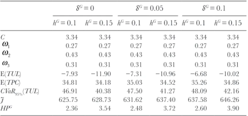
is the life annuity factor for age y after retirement T with t T= +1,T+2,…. Suppose the plan adopts the optimal asset allocation and normal contribution strategies shown in Table 8.5. Table 8.7 shows how the ground-up hedging strategy mitigates the funding downside risk caused by the capital market risk and longevity risk for the Base case with different hedge ratios.

With the ground-up hedging strategy, when hG_{>0, all}

CVaR95%(TUL)s in

Table 8.7 are lower than CVaR95%(TUL)=60 without hedging. Table 8.7 also

shows that as hG _{increases, CVaR TUL}

95%( ) and E(TPC) decrease, indicating a

lower pension risk to the plan. For example, when δG _{= 0, as h}G _{increases from 0.1}

to 0.15, CVaR_95%(TUL) decreases from 46.91 to 40.38 and E(TPC) decreases from

34.81 to 34.18. The hedge cost δG_{, however, reduces the risk reduction effect of the}

ground-up hedging. For example, when δG _{= 0 and h}G _{= 0.15, CVaR}

95%(TUL) is only

40.38 but it increases to 42.16 when δG _{= 0.1 and h}G _{= 0.15. As a robustness check,}

we also examine the ground-up hedging strategy with different combinations of g

and the pension asset parameters. All of them echo the pattern we observe in Table 8.7. We conclude that the ground-up hedging strategy can effectively reduce the capital market and longevity risks imbedded in a pension plan.

Table 8.7 Ground-up edging strategy for Base case with g = −0.2 δG _{= 0 δ}G _{= 0.05 δ}G _= 0.1 hG _{= 0.1 h}G _{= 0.15 h}G _{= 0.1 h}G _{= 0.15 h}G _{= 0.1 h}G _= 0.15 C 3.34 3.34 3.34 3.34 3.34 3.34 ω1 0.27 0.27 0.27 0.27 0.27 0.27 ω2 0.43 0.43 0.43 0.43 0.43 0.43 ω3 0.31 0.31 0.31 0.31 0.31 0.31 E(TUL) −7.93 −11.90 −7.31 −10.96 −6.68 −10.02 E(TPC) 34.81 34.18 35.03 34.52 35.26 34.86 CVaR_95%(TUL) 46.91 40.38 47.50 41.27 48.09 42.16 J 625.75 628.73 631.62 637.40 637.58 646.26 HPG _{2.36 3.54 2.48 3.72 2.60 3.90}

Note: C stands for the normal contribution. (ω1,ω2,ω1) represents the investment strategy

where ω2,ω2, andω3are the proportions invested in the S&P 500 index, Merrill Lynch

corporate bond index, and 3-month T-bill, respectively. g is the mortality improvement parameter in the Lee and Carter Model (1992). TUL and TPC represent the total unfunded liability and total pension cost of the plan. J is the value of the objective function in Model (5-13), which measures the variance of total unfunded liability. HPG_{, h}G_{, and δ}G _{are the}

hedge price, hedge ratio, and unit hedge cost under the ground-up hedging strategy. The Base case assumes the financial market maintains the same trend and volatility that it has demonstrated throughout the past 20 years.

The Excess-risk Hedging or Insurance Option Strategy

The second pension hedging strategy, the excess-risk hedging strategy, focuses on transferring the high-end longevity risk. With the excess-risk hedging strategy, the

plan needs to determine a strike level on the s-year survival probability s x Tp, for age

x at retirement T in each year t, t T= +1,T+2,… above which to transfer a

pro-portion hE _{of the longevity risk. The conditional expected s-year survival rate,} ˆ

,

spx T,

is defined as s x Tpˆ, =E p[s x T, px T, ,px+1,T+1, ,… px s+ −1,T s+ −1], wherepx s+ −1,T s+ −1is the

one-year survival rate for age x + s − 1 in year T + s − 1.

Suppose at t = 0, the plan purchases a series of European call options with strike

lev-els set at the expected survival rates, _{s x Tp,} =_{E p}[_{sx T,} ], 1 2_s= , ,_…. The option payoffs

in years T +1,T+2,… are determined by max{ ,0B psx T_, −B ps x T, },s=1 2, ,… .

Accordingly, to hedge a proportion hE_{, the plan needs to pay a hedge price of}

HPE h E v B p B p E E s s x T s x T s T =

(

+

)



{

−

}

 +

(

)

= ∞

∑

1 0 1 1 δ ρ max _, , ,

whereδE _{is the hedge cost per unit of longevity risk ceded. With the hedge ratio h}E_,

the plan’s liability becomes

PBO Ba x T Bh v p p t t E E s s x T s x T s T =

(

)

−

{

−

}

+

(

=

)

= ∞

∑

( ) max , , , , , , 0 1 1 2 1 … ρ TT Ba y BhE vs t T p p t T T s x T s x T s t T (t) ( )max , , , ,

( )

− − −

{

−

}

= + + = − + ∞

∑

₁ 0 1 22,…      

With the hedge price HPE_{, the fund available for investment at time 0 is reduced}

toME ₌M HP₋ E_{. Again, in our example, we assume M =5 and the pension}

plan implements the optimal asset allocation and normal contribution strategies

shown in Table 8.5. With different combinations of g and the pension asset

param-eters, we find the same pattern as Table 8.7 with the ground-up hedging strategy (results available on request from the authors). That is, with a positive hedge ratio

hE_,

CVaR95%(TUL) and E(TPC) are lower than those without hedge. However, the

magnitude of risk reduction achieved by the excess-risk hedging strategy is much

lower than that of the ground-up hedging strategy. For example, when g = −0.20,

the pension asset parameters in Table 8.1 andhG_{= 0.1, CVaR TUL}

95%( )=46 91.

with the ground-up hedging strategy. However, at the same levels of g and the

pension asset parameters, the excess-risk strategy only reduces CVaR95%(TUL)to

56.44 even with a full hedge of longevity risk above the expected survival rates (i.e.,

hE _{=1). This is explained by the fact that the excess-risk strategy only transfers the}

reduces both pension asset and liability risks. In many cases, the capital market risk on pension assets seems to impose a more significant effect on the pension plan than the longevity risk.

Conclusion

Concern regarding capital market risk often eclipses that due to longevity risk in pension management. When it comes to retirement issues, however, these two risks are integrally linked. The number of sustainable years for a retirement portfolio is determined, in part, by market crashes, changes in market volatility, and changes in life expectancy. There are instruments to handle capital market volatility, which include futures and forward contracts to hedge interest rate, currency, and price risks; there are also derivatives to hedge credit risks, weather risks, and more. There are insurance instruments to handle the volatility of life; these instruments include life insurance and life annuities. These insurance instruments have not, however, been designed to deal with the systematic component of the life risks. If life expec-tancy unexpectedly increases (e.g. a cure for cardiovascular disease or cancer is found), then life insurance becomes more profitable for the insurer but life annuities become less profitable, or may even threaten insurer solvency and adversely impact retirement plans of individuals and pension funds.

To address these issues, we created scenarios to assess risk for both the individ-ual and the institution. In the case of the individindivid-ual, scenario analysis showed that if the individual invested in a lifecycle fund such as that offered by TIAA-CREF and the financial markets were driven by historical parameters, then a $1 million investment at retirement combined with a withdrawal rate of $75,000 per year would yield approximately 20 sustainable years. This is one year more than the life expectancy of a 65-year-old male in 2013. Most financial planners would consider this as an inadequate retirement horizon, and many would advocate

planning for a much longer horizon.14 _{The same analysis shows that one could}

only say that the fund would last for ten years with a 99 percent probability. Similarly, if market parameters were doubled so that crashes occurred more often and the market was more volatile (i.e. BaseX2 case), one could expect the fund to last less than ten years and the fund would last for four years with 99 per-cent probability. This leaves the investor with considerable uncertainty. Yet the TIAA-CREF-type lifecycle fund held 40 percent in equity, 40 percent in bonds, and 20 percent in T-bills. The analysis also showed that the investor could select an alternative portfolio to increase the number of sustainable years. If the inves-tor held all in the bond fund, he could expect the portfolio to continue paying the same $75,000 per year for almost 35 years. Additionally, if the investor’s returns were in the worst 1 percent of the portfolio payoffs then he could still expect almost 18 sustainable retirement years, but only if the portfolio was changed to

a 30 percent investment in bonds and a 70 percent investment in T-bills. In the BaseX2 case (i.e. a more volatile market), the same investor could expect the port-folio fund to last almost 24 years if he plunged in the T-bill fund. In this BaseX2 case, if the investor’s returns were in the worst 1 percent of the portfolio payoffs then he could expect 11 sustainable retirement years, but only if the portfolio was altered to a 10 percent investment in bonds and a 90 percent investment in T-bills. These numbers do not account for the possible changes in life expectancy that will doubtless make even the best numbers here seem even less sufficient. The DC plans leave the investor with considerable longevity risk, and without the foresight of increasing the size of the investment fund they can only reduce the annual withdrawal or change the portfolio to attempt to keep the retirement fund sustainable for more years. These results emphasize the need for financial instru-ments that provide a more effective means of transferring some of the longevity risk to those better able to bear it.

Pension providers bear the longevity risk for DB plans. The pension provider has a fiduciary responsibility to act in the interest of the plan members and there-fore our scenario objective was to minimize pension underfunding subject to con-straints on the expected underfunding, short selling, and the size of the tail of the underfunding distribution. When longevity risk was increased, the solution to the constrained minimization problem showed an 8.3 percent increase in the expected total pension cost. When increased capital market risk was also added to longevity risk, the solution to the constrained minimization problem showed a 24.9 percent increase in the expected total pension cost.

To mitigate risk, two longevity risk-hedging schemes were considered. The first was similar to a partial buyout of the pension plan and the analysis showed that this hedge could lower the pension failure risk. When longevity risk was increased, the reduction in pension risk between the hedged and unhedged sce-narios became more pronounced; when capital market risk was also increased, the reduction in pension failure risk between the hedged and unhedged scenar-ios was even more pronounced. The second hedge was a longevity option. Here there was no exchange of assets; rather, there was only an exchange of liabilities in the tail. As was the case with the partial buyout strategy, the longevity option strategy also demonstrated a reduction in pension failure risk that increased with the size of the hedge.

In sum, improvements can result from managing longevity risk in the context of both defined contribution and defined benefit schemes. Today’s DC risk manage-ment schemes are currently far too limited (e.g. life annuities and reverse mort-gages, among others), and additional financial instruments can help fill the gap. The DB risk management possibilities are limited also, but they have received more attention in academia and in capital markets. Other hedging schemes must also be addressed.