Economic Performance of China (1980
–
2014)
Vivake Anand1* Dr. Jianhua Zhang2 Gulzar Ali3 Dr.Har Bakhsh Makhijani41 and 3. PhD Scholar, School of Economics,
2. Professor of Economics, Dean Peikang Chang Institute for Development Studies 1, 2 and 3. Huazhong University of Science and Technology, Wuhan, China
4. Assistant Professor, Department of Media and Communication Studies, University of Sindh, Jamshoro, Pakistan
Abstract
Success of Chinese economy has been well studied by now. This paper focuses on economic performance of China since 1980 to 2014. To measure economic performance of China, ‘Economic Performance Index’ (EPI) has been used. EPI uses four macroeconomic variables to calculate the EPI score. It was found that average EPI score for China in last 35 year is 96.49%, which is considered as overall excellent economic performance. Key words: Economic Performance, Growth, GDP, Inflation, Budget Deficit, China
Introduction
China has a long history of successful economic performance throughout centuries. The country has bestowed the world with magnificent innovations in science and arts. But, in last two centuries (i.e. 19th and 20th) the country went through civil unrest, wars and some major areas of the country were taken over by other nations. This caused over all down fall in the economic performance of the country. But soon after the World War II, China started to boom again, when Chairman Mao Zedong enthusiast-ed the people of China and developed a new social system within the country. This new social system imposed strict living rules upon civilians to maintain and minimize their living costs. After General Mao Zedong, his successor leader(s) continued his social system and also focused on market oriented strategies. It did not take too long to improve the living standard of local peoples in the country and, by 2000 GDP of China increase fourfold. Looking at this dramatic economic performance of China, Goldman Sachs15; in 2003, predicted that China will be the leading economy of the world by 2050 (Wilson, Purushothaman, & Goldman, 2003). And, in today’s circumstances it looks quite true. Today China has surpassed all developed economies; except USA, and stands second in the rank of GDP (WorldBank, 2014). China alone contributes to approximately 20% of world’s GDP16. This dramatic growth has captured minds of many researchers and there have been different studies about the growth and development in China. Many researchers including, Justin Yifu Lin and Zhiqiang Liu (2000) believe that roots of this growth lies in economic reforms that were in action since 1978.
In this paper we focus on economic performance of China. Our goal is to measure the economic performance of China since 1980s till 2014 on macro level. We have used an economic index called ‘economic performance index’ or ‘EPI’ to achieve our goal. This index was developed by Vadim Khramov and John Ridings lee17 in 2013. EPI uses four macroeconomic indicators that capture all three sectors; firm, households and government, of the economy. Variables of EPI include,
Inflation; (% change in CPI) measures monetary stability of economy. Unemployment; highlights production stance of economy.
Budget deficit as percentage of Total GDP; portrays fiscal strength of economy Percentage change in real GDP; reveals the overall performance of the economy.
15
Goldman Sachs is an American firm, dealing in investment banking and other financial securitization.
16
as per data collected on December 2014.
17
EPI Methodology
EPI calculation is very simple; rather than using heavy statistical methods, EPI comprises of simple arithmetic calculation. In normalized way EPI score is set to 100% and any decrease in this score is considered as decrease in economic performance of the country and vice versa. Generally, high inflations are considered negative for economic growth, but Federal reserve board (FRB) often requires central banks to maintain a minimum 2% rate of inflation over time to keep the economy moving (FRB, 2015). Following FRB requirements and available data, we have set desired value of inflation for China to 2%. In order to calculate EPI, we will subtract any value of inflation above our desired level of inflation from Standard EPI score (i.e. 100%). High unemployment rate indicated poor overall performance of economy. However, there is no optimal level of unemployment. But based on historical data we have set desired level of unemployment for China at 4% and will subtract the exceeded value from EPI score. Budget deficit exhibits the government’s ability to manage its expenditures against its revenues. In normal economic periods governments should maintain a policy at least to match revenue and expenditures (Khramov & Lee, 2013). As deficits are negative balances, and huge deficits indicates poor performance of the economy (Hakkio & Rush, 1991). For calculation of EPI in our research we have set desired budget deficit for China to 0%, and we will subtract any value of budget deficit from normal EPI score. On other hand, GDP growth indicates a positive attitude of economic performance. Many economists including Robert Solow18 and Tjalling Koopmans19 believe economies should try to achieve as high growth rates as possible. Economic growth opportunities vary from country to country, so the optimal growth rates also differ. In our study, based on available data and historical performance of China we have set desired GDP growth rate to 9%.
Mathematically EPI can be represented as;
Where Inf, UnE, BDef and ΔGDP represent inflation rate, unemployment rate, Budget deficit as percentage of GDP and percentage change in real GDP respectively and ‘*’ sign indicates desired values. Above equation concludes that when inflation rate deviates from its desired value it leaves a negative impact on EPI score (I.e. EPI falls when inflation rise). EPI also falls with the increase in unemployment rate and government deficits while it rises with positive GDP growth. But in times of high economic volatility this equation might give some messy picture of overall economic performance. So, in order to overcome this error and make EPI score comparable with other economies, Khramov and Lee (2013) have assigned weights to each variable used in above equations. Weights of each data variable are calculated by determining their inverse standard deviation and multiplying it with average standard deviation of all variables, so that, the sum of all weights equals to one. By doing this, resultant scores are smoothened and short-term economic trends and volatilities are easily captured. In our observations we found weighted EPI more flexible to economic trends and correlation between two indexes was 0.99; almost a perfect correlation. Equation for weighted EPI can be written as;
Where, Wi is weight assigned to each variable, and it is calculated by the formula;
Where StDi is standard deviation of every component used in weighted EPI equation and StDevAvis average
standard deviation of all the components. Formula for calculating average standard deviation is;
18
Robert Solow is well known economist who is popular for his work on growth theory
19
As, previously mentioned the average of weights equals 1. This weighting will help in maintaining same unit of measurement of all four components used in the model. Weighting approach used in this model is identical to the one implemented by Conference Board Coincident Economic Index® (CEI) and Chicago Fed National Activity Index (CFNAI).
Desired Inflation
Inflation is generally referred as tax on money or change in price of a given basket of good over specific time period. There are mainly two views about the inflation. First suggesting negative optimal inflation (Friedman, 1969), while other argues that there should be some small positive inflation to keep economy moving (Tobin, 1972). Friedman (1969), in his paper concluded that there should be no opportunity cost to individuals for holding their money, leading to idea of zero percent optimal interest rate, that will result in long term negative inflation. Standard neo-classical model of money also support the idea of negative optimal inflation (Kimbrough, 1986). Cash in advance framework used by Hodrick, Kocherlakota, and Lucas (1989), and findings of Chari, Christiano, and Kehoe (1996) agree with Friedman (1969) and support the idea of negative optimal inflation. While on other hand there are studies that suggest economies should maintain a small amount of inflation in order “to grease the wheels” and keep economies growing. Tobin (1972), studied the relationship between unemployment and inflation. He found that prices tend to increase in normal times and economies almost have some positive fraction of inflation. Similar kind of study was conducted by Kim and Ruge-Murcia (2009). They took a sample of U.S economy and found that minimum optimal inflation for U.S economy is 0.35% per annum. Using Keynesian model for U.S economy Billi (2011), found that optimal inflation for U.S ranges from 0.7% to 1.4%. Definitely, the optimal level of inflation varies from country to country depending upon the uncertainty within the economy. Fuchi, Oda, and Ugai (2008) while studying inflation in Japan found that optimal inflation for Japan should be 0.5% to 2.0%. Khramov and Lee (2013) in their paper have set the optimal inflation for all countries to zero. However, on the same time they have argued that this zero percent inflation rate may not be suitable for all economies. Growing economies may need higher inflation to maintain their growth.
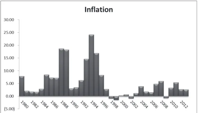
China being an emerging economy has maintained strict controls over inflation in last three years (i.e. 2012-2014), in these three years they have managed to maintain CPI below 3%. But, with the start of 2015 CPI increased 1.4% however producer price index (PPI) reduced 4.8% over previous year, as reported by BBC20. BBC also reported targeted inflation declined from 3.5% to 3% in 2015. In our sample of 35 year (1980 – 2014) China has witness high volatility in inflation. Figure 1, represents the inflation scenario in China for our selected period.
20
Figure 01: Inflation in China 1980-2014
Source; World Development Indicators, Global Economy, Trading economics.
According to data, inflation in China has been very volatile over time period of our study. Above figure shows that China has faced both; hyperinflation and deflation, within last 35 years. Descriptive values for inflation in China from 1980 t0 2014 are given in table 1. Descriptive analysis shows that 62.8% of our observation has values below 5% and 48.5% has values even below 3%. However, since 2000 China has made strict control over inflation. During financial crisis of 2007-2009 inflation rose to 5.9% followed by deflation -.070% in 2009. Keeping the idea of minimum optimal inflation and current performance of Chinese economy we conclude that China is still running a little over optimal rate of inflation. Thus, for our observations we set desired value for inflation to 2%.
Table 01: Discriptive(s) for Inflation in China 1980-2014
Min Max Mean Median Standard
Deviation Variance
-1.40 24.20 5.29 3.10 6.16 38.05
Desired Unemployment
Achieving zero percent unemployment is almost impossible for an economy. Economies often try to achieve full employment, which usually includes some fraction of labor force unemployed. This unemployment is due to emerging of new labor force, moving to better job etc. and is referred as natural rate of unemployment (NRU). Obliviously, large fraction of unemployed labor force is not considered good for economic growth. On other hand there is no determinant of optimal unemployment rate for an economy. Economies often design their employment polices based on NRU or non-accelerating inflation rate of unemployment (NAIRU) (Storm & Naastepad, 2012). Results obtained from NAIRU are used as targeted unemployment rate for current period. Values obtained from NAIRU change overtime, mainly due to two reasons. First, labor markets are highly unpredictable, having huge traffic. Second, interest conflicts; often referred as agency problem, between firms and employees that often lead to temporary unemployment (Blanchard & Katz, 1996). Various studies, including
Mitchell (1998) and Gordon (1996) found that value NAIRU changes from time to time depending upon different macro-economic factors like budget deficit, inflation etc..
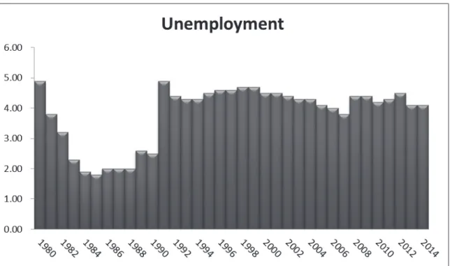
Figure 02: Unemployment in China 1980-2014
Historical, available data on unemployment in China suggest that China has maintained its overall unemployment rate below 5%. (see figure2). But, many studies, including (Knight & Xue, 2006; Liu, 2012) claim that urban unemployment in China is much higher that these figures. During a survey of five large cities of China, Giles, Park, and Zhang (2005) found that in 2002, 14% of permanent urban citizens were unemployed. While for China as whole, urban unemployment rose from 6.1% to 11.1% during 1996-2002 (Giles et al., 2005). However, general unemployment rates of China have been criticized by above mentioned authors, but in our study we will take unemployment values as given by World Bank and other databases21, as shown in figure 2. We also ignore NAIRU for setting up desired value of unemployment rate, because NAIRU changes overtime and is difficult to measure and depends on other factors (Ball & Mankiw, 2002). Descriptive analysis of above data shows that for last 35 years China has average unemployment of 3.83% while the median and standard deviation of data set are 4.30 and 0.99 respectively. Most of our observations on unemployment reveals that majority of data lie between 4%-5%. Keeping all these facts in mind we set desired value of unemployment in China to 4%, which is consistent with data and possibly achievable for China.
Desired Budget Deficit
Budget deficits/surplus exhibits government’s ability to manage its revenue against expenditure. Many studies; including (Choudhary & Parai, 1991; Metin, 1998) found that deficits in long run result in inflation. Some similar results were found by Dogas (1992) and Hondroyiannis and Papapetrou (1994). These studies show that governments are running current budget deficits on cost of future generation. Thus from above mentioned studies one can argue that governments should smooth their taxes and control its overall expenditures to run balanced budget overtime. However, there are some studies including (Sowa, 1994) that found budget deficit is not responsible for inflation neither in long-run nor in short. Another economist; William Vickrey, has criticized the idea that deficits cause future generation to suffer. In fact, he argues that “deficit is not economic sin but an economic necessity”. He argues that deficits adds value to our current purchasing power (Vickrey, 2000;
21
Vickrey, Vickrey, Rosen, & Vickrey, 1996). Other view about budget deficit suggests that government budget balances stabilize automatically. In recessions governments run budget deficits while in boom governments enjoy budget surplus (Khramov & Ridings Lee, 2013).
For China government budget balances; for last 35 years, vary from a surplus of 0.58% of GDP in 2007 to deficit of 3.05% of GDP in 1991. However, there is no clear conclusion about the impact and nature of budget deficits. We believe that government should manage their balances in long run. Thus, for our calculation of EPI we set desired value of budget deficit as 05 of GDP.
Desired GDP growth
GDP growth is often considered as growth of whole economy. There has been much debate and research on the determinants of economic growth. Robert. M, Solow, one of early economist, who came up with the idea that long-term economic growth depends upon the technological improvements and developed a model, now referred as Solow growth model (Solow, 1956). Solow growth model opened research gates for many researchers. Many researchers; including Cass (1965), used Solow’s growth model and found in steady state economy, technological improvements lead to overall economic growth in long-run. After that, ongoing debate upon growth economic and its determinants continued and different theories and model of exogenous and endogenous appeared. Some of these theories consider government size and fiscal policies as determinants of growth, while others consider tax and international trade, some suggest poor countries tend to grow faster, while others argue political and social framework within the country lead to long term growth (Bajo-Rubio, 2000; Barro & Lee, 1994; Easterly & Rebelo, 1993; Mankiw, Romer, & Weil, 1990).
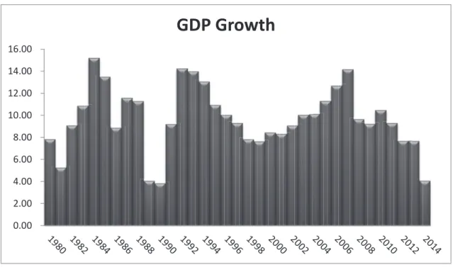
However, the opinions of economists vary about growth and its determinants, but most of them agree with the idea that higher growth rates preferable over lower ones because, higher growth rates ultimately lead to higher per-capita wealth in future. Data collected for China’s GDP growth rate; for last 35 years, shows that mean and median values are 9.7% and 9.3% respectively. It employs that in last three years China’s GDP has increased very rapidly. Furthermore, we found that 45.7% of observations had GDP growth rate over 10% and growth rate surpassed 9% in 65.7% observations (see figure 3). However, in past few years GDP growth has slowed down but, based on historical data and economic performance of China we have set desired GDP growth rate at 9%. Based on historical performance of China we argue that, this growth rate is not only desirable but also achievable for China.
Figure 03: GDP Growth in China during 1980-2014 0.00 2.00 4.00 6.00 8.00 10.00 12.00 14.00 16.00
GDP Growth
Economic Performance of China
We, agree with the fact that economic performance of China has been very volatile. In this section, we have analyzed historical performance of China using EPI index. We found that overall economic performance of China had been very good22 in last 35 years with average EPI score of 96.46 and weighted EPI score of 95.87. Figure 4, shows economic performance of China, measured by EPI. We found that both indexes follow similar pattern however, weighted EPI is more sensitive to economic trends. From Figure 4 we conclude that China has gone through rapid growth followed by sharp economic falls. In early days of 1980s, with implementation of new economic reforms economy of China got wings, resulting in excellent economic performance with EPI and weighted EPI score of 101.3% and 100.24% respectively. After 1985, China experienced some periods of higher inflation and GDP growth was comparatively lower than previous periods. This caused overall performance to decline, and EPI score fell from 101.3% in 1985 to 93.62% in 1989. In 1990 Chinese government introduced new market reforms, which gave more pace to Chinese economy and overall economic performance was smoothened. We found that average EPI score from 1990 – 2005 is 95.99%, which we consider as a good performance. In 2007, China ran a budget surplus of 0.58% of GDP with GDP growth rate of 14.16%, this boosted economic performance in this year resulting EPI score of 100.65%. During 2007-2009, whole world suffered of worst economic crisis of millennium and no doubt China was also hit by the turmoil and in following two years EPI declined sharply.
22
Figure 04: Overall Economic performance of China using EPI
In order to better communicate the results we have divided our selected time frame in to different periods. 1. Economic Reforms 1980-1989
After the death of Chairman Mao in 1976, Deng Xiaoping took the charge of China. He introduced economic reforms to country and relaxed the locals from tight, rigid control of government. Initially he focused on agriculture sector, giving anatomy to formers. According to this reform formers were liable to pay a share of their land’s output to government and could keep rest with them. This increased overall agricultural productivity and living standard of locals. On other hand, in early 1980s Deng established special economic zones in urban areas like Shantou; Shenzhen etc. these economic zones were assigned with special economic policies and were comparatively free from governmental interference and regulation. These region then became major source of economic growth as liberalized economic polices attracted many foreign investor. In order to improve industrial productivity Deng introduced ‘dual-price’ system throughout the country. Under this system domestic industries were allowed to produce and sell even above their regular quotas. Thus, increased productivity led consumers to enjoy more output. Private businesses were also encouraged to operate under dual price system and new business increased total output and created more jobs in economy.
Our observation for this period shows that economic reforms helped rapid growth in China but state also lost much of its revenue as a result of flexible economic policies. Tight control over inflation and increased GDP growth resulted in higher EPI score (table 2). But, due to flexible fiscal policies and increased money supply/flow, inflation rose dramatically after 1985. We found that EPI is capable of capturing these macro-economic changes. EPI score that reached to top of 101.3% in 1984 started to reduce with increase in inflation and reduced GDP growth. Thus in 1989 EPI score resulted as 93.63% (fair performance) with inflation rate of 18.3% and reduced GDP growth of 4.06%, which was reduced approximately four-fold since 1984. We found that overall/ average economic performance of China during 1980-1989 was excellent with average EPI score of 97.35% and weighted EPI score of 96.35%.
Table 02: Economic Performance of China during Economic reforms 1980-1989 Year Inflation Rate (%) Unemployment Rate (%) Budget Deficit (% 0f GDP) Change in Real GDP (%)
EPI (%) Grade Weighted
EPI (%) Grade 1980 7.90 4.90 1.65 7.84 94.06 B- 93.67 C+ 1981 2.10 3.80 1.65 5.24 95.47 B 94.84 B- 1982 1.80 3.20 1.65 9.06 97.64 A- 96.88 B+ 1983 1.70 2.30 1.65 10.85 99.45 A+ 98.47 A 1984 2.90 1.90 1.65 15.18 101.30 A+ 100.24 A+ 1985 8.50 1.80 1.65 13.47 99.95 A+ 98.79 A 1986 7.30 2.00 1.65 8.85 98.25 A 97.13 B+ 1987 7.20 2.00 1.65 11.58 99.23 A+ 98.13 A 1988 18.70 2.00 2.34 11.28 96.57 B+ 95.21 B 1989 18.30 2.60 2.06 4.06 93.62 C 92.42 D+ Average 7.23 2.64 1.85 9.20 97.35 A- 96.35 B+ Min 1.70 1.80 1.65 4.06 93.62 92.42 Max 18.70 4.90 2.34 15.18 101.30 100.24
2. Market and Education reforms 1990 – 1999
The protest of Tiananmen Square in 1989 ousted and threatened many of policy makers to reverse Deng’s reforms. But the reforms continued, and in 1992 Shanghai stock exchange and Shenzhen stock exchange were re-opened. Deng’s tour of southern China gave a new direction to Chinese economy. In this tour Deng emphasized on privatization and encouraged entrepreneurs to participate on new social market economy system. These social market economy reforms are one of key factor in China’s development today. He also made 9-year of education compulsory for individuals. New educational reforms for universities were introduced granting autonomy and flexibility to universities to improve higher education system. However, after his tour inflation rose to 14.6% in 1993 and 24.2% in 1994, because many of state owned companies were privatized and overall revenue of state reduced. However, GDP growth was still good and government was running a very low budget deficit of 0.8% in 1993. Our observations show that despite of high inflation, overall economy was growing and EPI score was above average (figure 4). In 1996 state maintained control over inflation and after death of Deng Xiaoping in 1997, most of state owned companies were liquidated and sold to private investors, banks were allowed to operate under relaxed policies, tariffs and quotas on cross border trade were reduced. This all helped control inflation and in 1998, peoples in China enjoyed deflation of 0.8%.
Figure 4, clearly portrays the economic trends during 1990-1999. The southern tour resulted in overall good performance of economy with EPI score of 98.04% (excellent economic performance), followed by downturn in economic performance due to higher inflation in 1993-1994. Thus, the reforms to control inflation and privatization of enterprises boosted overall economic performance and economy started to boom again in 1995. Re-acquisition of Hong Kong in 1997 and emergence of new private businesses restored confidence in the economy and overall economic performance was smoothened again in late 1990s. On average, we found that economic performance of China for this period was good with average EPI score of 95. 78% and weighted EPI score of 95.37%.
Table 03: Economic performance of China during 1990-1999
Year Inflation Unemployment
Budget Deficit (% of GDP) Change in Real GDP (%) EPI score (%) Grade Weighted EPI Score (%) Grade 1990 3.10 2.50 2.76 3.84 95.27 B 94.09 B- 1991 3.50 4.90 3.05 9.18 93.68 C+ 93.10 C- 1992 6.30 4.40 0.90 14.24 98.04 A 97.71 A- 1993 14.60 4.30 0.80 13.96 96.88 B+ 96.46 B+ 1994 24.20 4.30 1.10 13.08 94.74 B- 94.15 B- 1995 16.90 4.50 0.90 10.92 95.08 B 94.64 B- 1996 8.30 4.60 0.70 10.01 96.20 B+ 95.91 B 1997 2.80 4.60 0.70 9.30 96.81 B+ 96.57 B+ 1998 (0.80) 4.70 1.10 7.83 96.28 B+ 96.03 B+ 1999 (1.40) 4.70 1.90 7.62 95.42 B 95.03 B Average 7.47 4.55 1.39 10.46 95.78 B 95.37 B Min (1.4) 2.50 0.7 3.84 93.68 93.10 Max 24.20 4.90 3.05 14.24 98.04 97.71
3. China as Global Player 2000-2014
After joining World Trade Organization in 2001, China appeared as a global player in world economy. Well maintained control over inflation, higher GDP growth rates and large scale privatization attracted more of the business from rest of world. By 2004, international trade policies were further relaxed attracting more business. Large scale privatization increased overall productivity of the country, and in 2005 contribution of domestic private companies to GDP exceeded 50% of total GDP and continues to increase still today (Schoenleber, 2006). During 2001 – 2004 tariffs were further reduced and banks system was reformed. All these reforms all together enabled China to become largest economy in Asia in 2005. However, in late 2005 few of Deng’s reforms were reversed. State halted further privatization and government adopted much loose monetary policy, which resulted in housing price boom in 2007. New system since 2005 focused much on health care and establishment of
“national champions” and make them able to compete the world, rather than relying on the investments from private sector.
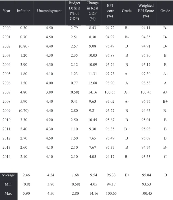
Beginning of new millennium proved good for Chinese economy, it was found that since 2000 economic performance of china increased and reached to top score of 100.65% (superior performance) in 2007(figure 4). Reversal of Deng’s reforms, loose monetary policies and global financial crisis of 2007-2009 put negative effect(s) on overall economic performance. In 2009, EPI score reduced to 95.27% (good performance) and has further reduced in recent years to 94.74% (fair performance) in 2013 and 93.53% (fair performance) in 2014. Despite of relatively poor performance in last three years, it was found that; on average, economy of China has resulted in overall good economic performance for this period.
Table 04: Economic performance of China 2000-2014
Year Inflation Unemployment
Budget Deficit (% of GDP) Change in Real GDP (%) EPI score (%) Grade Weighted EPI Score (%) Grade 2000 0.30 4.50 2.79 8.43 94.72 B- 94.11 B- 2001 0.70 4.50 2.51 8.30 94.92 B- 94.35 B- 2002 (0.80) 4.40 2.57 9.08 95.49 B 94.91 B- 2003 1.20 4.30 2.35 10.03 95.88 B 95.30 B 2004 3.90 4.30 2.12 10.09 95.74 B 95.17 B 2005 1.80 4.10 1.23 11.31 97.73 A- 97.30 A- 2006 1.50 4.00 0.77 12.68 98.90 A 98.53 A 2007 4.80 3.80 (0.58) 14.16 100.65 A+ 100.45 A+ 2008 5.90 4.40 0.41 9.63 97.02 A- 96.75 B+ 2009 (0.70) 4.40 2.80 9.21 95.27 B 94.65 B- 2010 3.30 4.20 2.50 10.45 95.67 B 95.01 B 2011 5.40 4.30 1.10 9.30 96.35 B+ 95.93 B 2012 2.70 4.50 1.50 7.65 95.49 B 95.07 B 2013 2.60 4.10 2.10 7.67 95.37 B 94.74 B- 2014 2.10 4.10 2.10 4.05 94.17 B- 93.53 C Average 2.46 4.24 1.68 9.54 96.33 B+ 95.84 B Min (0.8) 3.80 (0.58) 4.05 94.17 93.53 Max 5.90 4.50 2.80 14.16 100.65 100.45
Conclusion
Since 1978, implementation of economic reform in China has caused economic growth in China. In early 1980s market oriented strategies and privatization of state owned enterprises resulted on overall increased output and since then China started to boom. To measure economic performance of China, we used EPI and Weighted EPI and found that despite of heavy fluctuation in economic conditions in last 35 years average economic performance of China has been very good with EPI score of 96.46%. Privatization in early days increased confidence among investors and entrepreneurs. Emergence of new business caused more jobs and contributed to overall GDP. Famous southern tour of Deng Xiaoping in 1992 created more confidence in economy and fiscal and trade polices with further relaxed that increased overall performance. However in 1993, flexible monetary policies caused inflation to rise and reduced total EPI score for short time. In 2001, China joined WTO and was open to international trade. Flexible trade polies and reduced tariffs helped attract more business from other economies, this caused government revenues and GDP growth rate to increase thus EPI score was further enhanced. Property price bubble in 2007 and global financial crisis of 2007-2009 has however, left a negative impact on EPI score in recent year. But, on average; we conclude, that economic performance of China has been very good.
References
Bajo-Rubio, O. (2000). A further generalization of the Solow growth model: the role of the public sector.
Economics Letters, 68(1), 79-84. doi: http://dx.doi.org/10.1016/S0165-1765(00)00220-2
Ball, L., & Mankiw, N. G. (2002). The NAIRU in Theory and Practice. National Bureau of Economic Research Working Paper Series, No. 8940. doi: 10.3386/w8940
Barro, R. J., & Lee, J.-W. (1994). Sources of economic growth. Carnegie-Rochester Conference Series on Public Policy, 40(0), 1-46. doi: http://dx.doi.org/10.1016/0167-2231(94)90002-7
Billi, R. M. (2011). Optimal inflation for the US economy. American Economic Journal: Macroeconomics, 29-52.
Blanchard, O., & Katz, L. F. (1996). What We Know and Do Not Know About the Natural Rate of Unemployment. National Bureau of Economic Research Working Paper Series, No. 5822. doi: 10.3386/w5822
Cass, D. (1965). Optimum Growth in an Aggregative Model of Capital Accumulation. The Review of Economic Studies, 32(3), 233-240. doi: 10.2307/2295827
Chari, V. V., Christiano, L. J., & Kehoe, P. J. (1996). Optimality of the Friedman rule in economies with distorting taxes. Journal of Monetary Economics, 37(2), 203-223.
Choudhary, M. A. S., & Parai, A. K. (1991). Budget deficit and inflation: the Peruvian experience. Applied Economics, 23(6), 1117-1121. doi: 10.1080/00036849100000015
Dogas, D. (1992). Market power in a non-monetarist inflation model for Greece. Applied Economics, 24(3), 367-378. doi: 10.1080/00036849200000150
Easterly, W., & Rebelo, S. (1993). Fiscal policy and economic growth. Journal of Monetary Economics, 32(3), 417-458. doi: http://dx.doi.org/10.1016/0304-3932(93)90025-B
FRB. (2015, January 26, 2015). Why does the Federal Reserve aim for 2 percent inflation over time? Current
FAQs. Retrieved April 03, 2015, from http://www.federalreserve.gov/faqs/economy_14400.htm
Friedman, M. (1969). The optimum quantity of money, and other essays.
Fuchi, H., Oda, N., & Ugai, H. (2008). Optimal inflation for Japan's economy. Journal of the Japanese and international economies, 22(4), 439-475.
Giles, J., Park, A., & Zhang, J. (2005). What is China's true unemployment rate? China Economic Review, 16(2), 149-170. doi: http://dx.doi.org/10.1016/j.chieco.2004.11.002
Gordon, R. J. (1996). The Time-Varying NAIRU and its Implications for Economic Policy. National Bureau of Economic Research Working Paper Series, No. 5735. doi: 10.3386/w5735
Hakkio, C. S., & Rush, M. (1991). IS THE BUDGET DEFICIT “TOO LARGE?”. Economic Inquiry, 29(3), 429-445. doi: 10.1111/j.1465-7295.1991.tb00837.x
Hodrick, R. J., Kocherlakota, N. R., & Lucas, D. J. (1989). The variability of velocity in cash-in-advance models: National Bureau of Economic Research Cambridge, Mass., USA.
Hondroyiannis, G., & Papapetrou, E. (1994). Cointegration, causality and the government budget-inflation relationship in Greece. Applied Economics Letters, 1(11), 204-206. doi: 10.1080/135048594357880
Justin Yifu Lin, & Zhiqiang Liu. (2000). Fiscal Decentralization and Economic Growth in China. Economic Development and Cultural Change, 49(1), 1-21. doi: 10.1086/452488
Khramov, V., & Lee, J. R. (2013). The Economic Performance Index (Epi): An Intuitive Indicator for Assessing a Country's Economic Performance Dynamics in an Historical Perspective: International Monetary Fund.
Khramov, V., & Ridings Lee, J. (2013). The Economic Performance Index (EPI): an Intuitive Indicator for Assessing a Country's Economic Performance Dynamics in an Historical Perspective.
Kim, J., & Ruge-Murcia, F. J. (2009). How much inflation is necessary to grease the wheels? Journal of
Monetary Economics, 56(3), 365-377. doi: http://dx.doi.org/10.1016/j.jmoneco.2009.03.004
Kimbrough, K. P. (1986). The optimum quantity of money rule in the theory of public finance. Journal of
Monetary Economics, 18(3), 277-284. doi: http://dx.doi.org/10.1016/0304-3932(86)90040-1
Knight, J., & Xue, J. (2006). How High is Urban Unemployment in China? Journal of Chinese Economic and Business Studies, 4(2), 91-107. doi: 10.1080/14765280600736833
Liu, Q. (2012). Unemployment and labor force participation in urban China. China Economic Review, 23(1), 18-33. doi: http://dx.doi.org/10.1016/j.chieco.2011.07.008
Mankiw, N. G., Romer, D., & Weil, D. N. (1990). A Contribution to the Empirics of Economic Growth. National Bureau of Economic Research Working Paper Series, No. 3541. doi: 10.3386/w3541 Metin, K. (1998). The Relationship Between Inflation and the Budget Deficit in Turkey. Journal of Business &
Economic Statistics, 16(4), 412-422. doi: 10.1080/07350015.1998.10524781
Mitchell, W. F. (1998). The Buffer Stock Employment Model and the NAIRU: The Path to Full Employment. Journal of Economic Issues, 32(2), 547-555. doi: 10.2307/4227333
Schoenleber, H. (2006). CHINA’S PRIVATE ECONOMY GROWS UP. Retrieved from 8km | Know More website: http://8km.de/2006/19/
Solow, R. M. (1956). A Contribution to the Theory of Economic Growth. The Quarterly Journal of Economics, 70(1), 65-94. doi: 10.2307/1884513
Sowa, N. K. (1994). Fiscal deficits, output growth and inflation targets in Ghana. World Development, 22(8), 1105-1117. doi: http://dx.doi.org/10.1016/0305-750X(94)90079-5
Storm, S., & Naastepad, C. W. M. (2012). Macroeconomics beyond the NAIRU. Harvard University Press. Tobin, J. (1972). Inflation and unemployment. American economic review, 62(1), 1-18.
Vickrey, W. (2000). We Need a Bigger ‘Deficit.’.
Vickrey, W., Vickrey, C., Rosen, S., & Vickrey, W. S. (1996). FIFTEEN FATAL FALLACIES OF FINANCIAL FUNDAMENTALISM.
Wilson, D., Purushothaman, R., & Goldman, S. (2003). Dreaming with BRICs: the path to 2050 (Vol. 99): Goldman, Sachs & Company.
WorldBank. (2014). GDP Ranking. Retrieved 2015-03-31, from World Bank http://data.worldbank.org/data-catalog/GDP-ranking-table
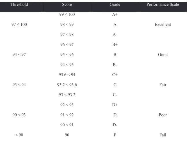
Appendix - A: Grading EPI Score.
We have adopted similar technique to Khramov and Ridings Lee (2013), to grade our resultant EPI scores. Based on our data and results we have designed following table to assign grades and ranks to EPI score.
Table 5 EPI Grading/Scaling System
Threshold Score Grade Performance Scale
97 ≤ 100 99 ≤ 100 A+ Excellent 98 < 99 A 97 < 98 A- 94 < 97 96 < 97 B+ Good 95 < 96 B 94 < 95 B- 93 < 94 93.6 < 94 C+ Fair 93.2 < 93.6 C 93 < 93.2 C- 90 < 93 92 < 93 D+ Poor 91 < 92 D 90 < 91 D- < 90 90 F Fail
Appendix - B: Normalizing Data.
During our observation we found datasets very volatile. It was very difficult to reach a meaningful conclusion about EPI score with such versatile data. In order to bring data under observation we used normalized data, rather than actual one. We have brought data in same scale of 1 to 5. Data is normalized in such a way that both, actual and normal data follows similar trends. Data in normalize with following formula;
where,
= normalized variable = actual variable
= normalized dataset minimum = normalized data set maximum
= actual dataset minimum = actual data set maximum.