Efficient Remote Profiling
for Resource-Constrained Devices
Priya Nagpurkar, Hussam Mousa, Chandra Krintz, and Timothy Sherwood University of California, Santa Barbara
{priya,husmousa,ckrintz,sherwood}@cs.ucsb.edu
The widespread use of ubiquitous, mobile, and continuously-connected computing agents has inspired software developers to change the way they test, debug, and optimize software. Users now play an active role in the software evolution cycle by dynamically providing valuable feedback about the execution of a program to developers. Software developers can use this information to isolate bugs in, maintain, and improve the performance of a wide-range of diverse and complex embedded device applications. The collection of such feedback poses a major challenge to systems researchers since it must be performed without degrading a user’s experience with, or consuming the severely restricted resources of the mobile device. At the same time, the resource constraints of embedded devices prohibit the use of extant software profiling solutions.
To achieve efficient remote profiling of embedded devices, we couple two efficient hardware/soft-ware program monitoring techniques: Hybrid Profiling Support(HPS) and Phase-Ahardware/soft-ware Sampling. HPS efficiently inserts profiling instructions into an executing program using a novel extension to Dynamic Instruction Stream Editing(DISE). Phase-aware sampling exploits the recurring behavior of programs to identify key opportunities during execution in order to collect profile information (i.e. sample). Our prior work on phase-aware sampling required code duplication to toggle sampling. By guiding low-overhead, hardware-supported sampling according to program phase behavior via HPS, our system is able to collect highly accurate profiles transparently.
We evaluate our system assuming a general purpose configuration as well as a popular hand-held device configuration. We measure the accuracy and overhead of our techniques and quantify the overhead in terms of computation, communication, and power consumption. We compare our system to random and periodic sampling for a number of widely used performance profile types. Our results indicate that our system significantly reduces the overhead of sampling while maintaining high accuracy.
Categories and Subject Descriptors: C [3]: 0—Computer Systems Organization - Special-Purpose and Application-Based Systems
General Terms: Performance
Additional Key Words and Phrases: profiling, sampling, resource-constrained devices, phased behavior
1. INTRODUCTION
The explosive growth and widespread use of the Internet has precipitated a signifi-cant change in the way that software is bought, sold, used, and maintained. Users are no longer disconnected individuals that passively execute disks from a shrink-wrapped box, but are instead often far more involved in the software development and improvement process. Users currently demand bug fixes, patches, upgrades, forward compatibility, and security updates served to them over the ever-present network. Moreover, this ubiquity of access allows usersto participate directlyin the evolution process of deployed software. Users currently transmit error reports upon program failure in modern operating systems [MicrosoftErrorReporting ] and allow remote monitoring of their applications by software engineers for use in coverage
testing [Orso et al. 2002] and bug isolation [Liblit et al. 2003].
The goal of our work is to extend remote monitoring so that it can be used on resource-constrained devices, e.g., hand-helds and cellular phones, and to in-vestigate its efficacy for performance profiling. Performance profiling offers soft-ware engineers a unique opportunity to employ feedback from actual users to guide program optimizations that improve software performance and minimize resource consumption. Such optimization is vital since mobile device software has become increasingly complex and is commonly released with performance bottlenecks or in-sufficient optimization, since developers cannot know exactly how the software will be usedin the wild. This problem is compounded by the infeasibility of providing extensive testing and optimization for all possible device configurations on which the programs will run.
In this paper, we present a hardware/software system for efficient remote per-formance profiling of resource-constrained systems. Our system collects sample-based profiles of program execution from user devices and transmits them back to an optimization center for analysis, possible re-coding, and re-compilation using feedback-based optimization, as part of the software evolution process.
Our system samples the program execution stream by turning profiling on and off dynamically (i.e. toggling) using Hybrid Profiling Support (HPS). HPS is an extension of dynamic instruction stream editing (DISE) [Corliss et al. 2003b] a hardware approach for macro-expansion, i.e., automatic replacement of executing instructions. HPS is very flexible (similar to extant software sampling systems) in that it can implement a wide-range of different profile types and sampling scenarios dynamically (e.g., random, periodic, and program-aware [Arnold and Ryder 2001]) via a flexible software interface. In addition, HPS is highly efficient (similar to extant hardware sampling systems) since it does not require code duplication or impose any overhead other than for the execution of the instructions required for profile collection (instrumentation).
We couple HPS with a novel and intelligent mechanism for toggling profile col-lection that achieves efficiency and accuracy through the exploitation of program phases. Using program phase behavior, we can summarize a software system as a minimal but diverse set of program behaviors in a manner that is distributed, dynamic, efficient, and that accurately reflects overall program behavior. This phase-aware mechanism also consists of both hardware and software components. The hardware efficiently monitors program execution behavior and makes predic-tions about when a new phase will occur. A software profiling daemon triggers HPS sample collection for eachpreviously unseen phase.
Our work contributes a system that combines hybrid profiling support and phase-aware sampling. Prior to this work, phase-phase-aware sampling relied on code duplica-tion to enable toggling of profile collecduplica-tion. HPS enables us to avoid code dupli-cation and to implement efficient phase sampling that imposes overhead only for the instrumentation instructions that collect the profile dataduring sampling. We describe how we combine these systems and use them study a number of different profile types that were previously shown to be important for feedback-directed op-timization, e.g. hot methods, hot call pairs, and hot code regions. We evaluate both the profile accuracy and overhead of our system and compare our approach to commonly used periodic and random sampling strategies using a wide range of
benchmarks (those developed for general purpose as well as embedded systems). We also evaluate the efficiency and battery consumption of our system for a resource-constrained environment. We consider both the computation and communication required for remote profile collection and its transmission to an optimization center. In the sections that follow, we first overview extant approaches to program sam-pling in hardware and software. We then describe our remote profiling system and its two primary components: Hybrid Profiling Support and Phase Aware Sampling. We then detail the design and implementation of each of these components in sec-tions 3 and 4, respectively. Finally, we present an extensive empirical evaluation of our system in section 5 and conclude in section 6.
2. PROGRAM SAMPLING
The goal of our work is efficient performance profiling using a combination of hard-ware and softhard-ware. We focus on techniques for the collection of incomplete infor-mation about program execution, i.e. program sampling. Sampling introduces less overhead than exhaustive profile collection at a cost of reduced profile accuracy. Profile accuracy is the degree to which a sample-based profile is similar to a com-plete, exhaustive profile. Sample-based profiling systems attempt to achieve the highest accuracy with the least overhead.
Sample-based techniques have been shown to be effective when implemented in either hardware or software. Examples of hardware-based profiling systems include custom hardware that collects specific profile types [Dean et al. 1997; Gordon-Ross and Vahid 2003; Heil and Smith 2000; Merten et al. 1999], systems that utilize existing hardware to collect application-specific performance data [Anderson et al. 1997; Itzkowitz et al. 2003; Peri et al. 1999], and programmable co-processors for profiling [Zilles and Sohi 2001] and profile compression [Sastry et al. 2001].
These approaches require no modification to application code, are highly efficient, and in most cases, avoid adverse, indirect performance effects such as memory hi-erarchy pollution. The disadvantage to such approaches in addition to increased hardware complexity and die area, is a lack of flexibility, i.e., the inability or dif-ficulty to re-program the hardware. For example, most approaches implement a single profile type, e.g., instructions executed, branches, or memory accesses.
Software sampling systems offer improved flexibility, portability, and accuracy over hardware-based systems. Moreover, software systems can collect application-specific information easily without help from the operating system since they oper-ate at a much higher level of abstraction. Hardware systems, on the other hand, col-lect full system profiles, i.e., they are program-agnostic. Software systems, however, suffer from additional limitations. In particular, software systems introduce signif-icant overhead due to the instrumentations that gathers profile data and decides when to sample. Moreover, software profiling systems introduce indirect overhead in the form of memory hierarchy pollution, increased virtual memory paging, and frequent CPU pipeline stalling. In addition to degrading performance, the indirect effect of the profiling instrumentation can change the runtime application behavior and further reduce the accuracy of the gathered information.
To design a sample-based profiling system we must answer three primary ques-tions: (1) how to toggle profiling on and off, (2) when to sample, and (3) how long to sample. One way to answer the first question is to simply insert the
instrumen-tation necessary to collect a profile of the events of interest immediately prior to all such events in the program [Grove et al. 1995; H¨olzle and Ungar 1994]. We can perform such instrumentation at the source, bytecode, or binary level.
One method that reduces the overhead of thisexhaustive instrumentationis code patching [Suganuma et al. 2002; Tikir and Hollingsworth 2002; Traub et al. 2000]. Code patching is a dynamic instrumentation technique that modifies the execut-ing program binary to execute (or stop executexecut-ing) the code for profile collection. In [Suganuma et al. 2002] for example, the compilation system inserts instrumen-tation into the prolog of methods. The instrumeninstrumen-tation is a call to a procedure that records method invocation (call path) events. After a fixed number of method invocations (samples), the system overwrites the profiling instructions so that fu-ture invocations execute unimpeded; eliminating all profiling overhead for uninstru-mented code. Unfortunately, code patching is error prone, significantly complicates the compilation and runtime system, and the process can impose additional over-heads (e.g. to flush the instruction cache).
An alternative approach to dynamic instrumentation for software sampling em-ploys code duplication [Arnold and Ryder 2001; Hauswirth and Chilimbi 2004; Hirzel and Chilimbi 2001; Nagpurkar et al. 2005]. Such systems duplicate some or all of the program binary (bytecode or native executable). The system inserts instrumentations into the duplicate copy to collect the appropriate profile type(s), e.g. hot methods, memory accesses, etc. The original copy is also instrumented with a set of counters that decide when to transition to the instrumentedprofiling code region. The system inserts these instrumentations at compile time [Arnold and Ryder 2001; Nagpurkar et al. 2005], or at load time via static binary instru-mentation [Hirzel and Chilimbi 2001; Hauswirth and Chilimbi 2004].
To decide when to sample, sampling systems commonly employ random or pe-riodic sampling intervals [Sastry et al. 2001; Liblit et al. 2003; Orso et al. 2002; Whaley 2000; Arnold et al. 2000; Hazelwood and Grove 2003; SunHotSpot ; Arnold et al. 2000; Cierniak et al. 2000]. Random sampling ensures that samples are statis-tically distributed over the execution of a program. Periodic sampling systems turn profile collection on using timer interrupts from the execution environment. The frequency with which periodic and random samples are taken, however, does not account for repeating patterns in program execution. As a result, such schemes can collect redundant profile information and can miss important events (code regions) completely.
Other sampling systems attempt to sample more intelligently – according to the dynamic program behavior [Arnold and Ryder 2001; Hirzel and Chilimbi 2001; Hauswirth and Chilimbi 2004; Arnold and D.Grove 2005; Nagpurkar et al. 2005]. Such systems employ the code duplication model described above. These systems insert instructions in the uninstrumented code that manipulate counters to cause control to transfer to the instrumented copies when a threshold is reached. We re-fer to the overhead that these checks impose as thebasic overhead. Basic overhead is introduced by these sampling systems constantly, regardless of weather profile information is actually being collected. Basic overhead accounts for 1-10% of ex-ecution time in a Java virtual machine sampling system [Arnold and Ryder 2001] and 6-35% in a binary instrumentation system (3-18% using overhead reduction techniques that reduce the number of dynamic checks) [Hirzel and Chilimbi 2001].
The final question a sampling system must answer is how long to profile once sampling commences. Random and periodic sampling systems commonly collect information about a single event [Whaley 2000], an intelligent set of events [Arnold and D.Grove 2005], or a fixed set of events (e.g. instructions or branches executed) immediately following the sampling trigger [Nagpurkar et al. 2005]. Systems that rely on code duplication to toggle profile collection, commonly execute within the instrumented code for a single pass (until the next loop back-edge or method in-vocation) [Arnold and Ryder 2001; Mousa and Krintz 2005] or for multiple passes depending upon the profile type [Hirzel and Chilimbi 2001; Hauswirth and Chilimbi 2004; Mousa and Krintz 2005].
2.1 Our Approach
As we describe above, each existing approach to program sampling has its strengths and weaknesses. Hardware approaches are inflexible in terms of their configuration and types of profiles they collect. Software approaches enable flexibility but can introduce significant overhead or employ methodologies that are infeasible for re-source constrained devices, e.g., code duplication. To address these limitations, we designed a novel sampling system that combines and extends extant technologies in a way that is appropriate for embedded systems such as cellular phones and personal digital assistants (PDAs). The goal of our work is to enable remote per-formance profiling of deployed software in these environments that is transparent, efficient, and accurate.
The profiling system that we propose uses a hardware/software (hybrid) approach for its implementation. It consists of two main components: Hybrid Profiling Sup-port(HPS) andPhase-Aware Sampling. HPS employs dynamic instruction stream editing [Corliss et al. 2003b] to turn profile collection on and off, i.e., to sample the executing instruction stream.
To enable efficient remote collection of accurate profile information, our mech-anism for deciding when to sample (i.e., when to turn on HPS profile collection) exploits program phase information. The way a program’s execution changes over time is not random, but is often structured into repeating behaviors, i.e., phases. Using the description of phases from our previous work [Sherwood et al. 2001], a phase is a set of dynamic instructions(intervals) during program execution that have similar behavior, regardless of temporal adjacency. Prior work [Sherwood et al. 2001; Sherwood et al. 2002; Sherwood et al. 2003; Dhodapkar and Smith 2002; Duesterwald et al. 2003] has shown that it is possible to identify, predict, and create meaningful classifications of phases in program behavior accurately. Phase behavior has been used in the past to reduce the overhead of architectural simulation [Sher-wood et al. 2002; Pereira et al. 2005] and to guide online optimizations [Dhodapkar and Smith 2002; Duesterwald et al. 2003; Sherwood et al. 2003].
In this paper, we employ program phase behavior in a novel way: to identify intelligently a representative set of profiling points. The advantage we gain by using phase information is that we only need to gather information about part of the phase and then use that information to approximate overall profile behavior. By carefully selecting a representative from each phase, we can drastically reduce the number of times that we need to sample and the amount of total communication required for profile transmission to the optimization center. Since an interval will
0 1 2 3 4 5 Instructions Executed (Billions)
0.0 0.1 0.2 0.3 0.4 uJ/Instr
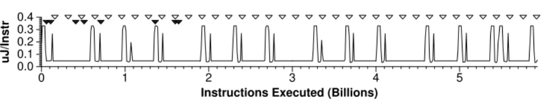
Fig. 1. The figure shows the run-time power usage of the full execution of the programmpeg encode.The program exhibits different phases, marked by periods of high and low power. A random or periodic sampling method (the white triangles) will continue to take samples over the full execution of the program. A more intelligent sampling technique based on phase information (shown as black triangles) can achieve the same profile accuracy, by taking fewer key samples from each phase.
be similar to all other intervals in a phase, it can serve as a representative of the entire phase. As such, only select intervals of the program’s phases need to be collected (instrumented, communicated, and analyzed) in order to capture the behavior of the entire program. This will make more efficient use of those limited resources available on mobile devices. Furthermore, these low-overhead profiles will be highly accurate (very similar to exhaustive profiles of the same program).
Figure 1 exemplifies our approach using actual energy data gathered from the execution of the mpeg encoding utility. The execution of mpeg exhibits a small number of distinct phases during execution that repeat multiple times. A random or periodic sampling method will continue to take samples over the full execution of the program regardless of any repeating behavior. In Figure 1, the white triangles show where samples would be taken if sampling is done periodically to achieve an accuracy error of 5% (i.e. the resulting basic block count profile is within 5% of the exhaustive profile). This has the unfortunate drawback that mostof the samples will not provide any new information because they are so similar to samples seen in the past. A more intelligent sampling technique based on phase information (shown as black triangles) can achieve the same error rate with significantly fewer samples. This is done by taking only key samples from each phase.
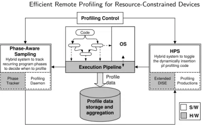
Figure 2 provides an overview of the interactions among the primary components of our system. The phase-aware sampler consists of a hardware phase tracker that monitors the execution stream and predicts, for each interval in the program, whether the interval is in a previously seen or unseen phase. A software profiling daemon triggers profile collection by the hybrid profiling support (HPS) system for representative intervals from as-yet-unsampled phases. We can also trigger collection directly via a connection between the phase tracker and HPS; we avoid this approach since it restricts flexibility and system modularity.
HPS intercepts the instruction stream to dynamically insert instrumentation code for instructions of interest (those to be profiled) when its sampling flag is set by the phase-aware sampler. At the end of an interval, the profiling daemon clears the HPS sampling flag and all instructions execute unimpeded. The system stores samples locally for aggregation and transmission by the profiling daemon to the optimization center, as needed. In the sections that follow, we first detail the HPS system (section 3) and then present phase-aware profiling and the interaction of these two components (section 4).
Execution Pipeline OS Profile data Profile data storage and aggregation Code HPS Hybrid system to toggle the dynamically insertion
pf profiling code Extended
DISE ProductionsProfiling
Phase-Aware Sampling Hybrid system to track recurring program phases
to decide when to profile Phase
Tracker ProfilingDaemon
Profiling Control
S/W H/W
Fig. 2. Overview of the main components of our efficient profiling system for remote embedded devices. The HPS system (section 3) is responsible for the dynamic insertion and toggling of profiling instructions. The phase tracking system (section 4) is responsible for deciding when to gather profile information.
3. HYBRID PROFILING SUPPORT FOR TOGGLING PROFILE COLLECTION To efficiently toggle profile collection, our system employs HPS, a hardware/software (hybrid) approach for dynamic profiling. HPS is an application and extension of Dynamic Instruction Stream Editing(DISE) [Corliss et al. 2003b]. DISE is a hard-ware mechanism that dynamically and transparently inserts instructions into the execution stream thereby enabling semantics similar to macro expansion in the C programming language.
Figure 3 is an overview of our HPS design. HPS consists of an extension to DISE (dark grey region in the hardware (H/W) section) that enables highly efficient, con-ditional, dynamic profile collection. HPS supports the toggling of profile collection via external triggers such as timer interrupts or periodic events. HPS also includes an internal flexible, program driven, triggering mechanism based on the sampling framework proposed by [Arnold and Ryder 2001] and extended by [Hirzel and Chilimbi 2001]. Furthermore, HPS enables the profile consumer to specify arbi-trary instructions of interest and associate them with profile collection actions via HPS and DISE based semantics. We next overview the DISE system and then describe how we extend DISE and apply it for efficient profiling in HPS.
3.1 Dynamic Instruction Stream Editing (DISE)
Hardware architects implement dynamic instruction stream editing by extending thedecodestage of a processor pipeline. The extensions identify interesting instruc-tions and replace them with an alternate stream of instrucinstruc-tions.
To enable this, DISE stores encoded instruction patterns and pdecoded re-placement sequences in individual DISE-private SRAMs calledthe pattern table (PT)andthe replacement table (RT)respectively. The hardware compares (in parallel) each instruction that enters the decode stage against the entries in the PT. On a match, DISE replaces the original instruction with an alternate stream of instructions that commonly includes the original instruction. DISE retrieves this stream of instructions from the RT according to an index generated by the PT.
Execution Pipeline Application Sample Trigger Mechanism DISE with HPS extensions Profile
Specifications ParametersProfiling Profile
Consumer S/W
H/W
Fig. 3. The Hybrid Profiling Support (HPS) system. HPS contains a hardware component which is an extension of Dynamic Instruction Stream Editing(DISE). Software level mechanisms control the profiling framework and provide facilities for the profile consumer to define their profiling specifications (including instructions of interest and actions to be taken). HPS allows the profile consumer to set the profiling strategy (e.g. triggering policy – exhaustive, periodic, program driven, ...) and control the profiling parameters.
An Instantiation Logic (IL) unit is employed by DISE to parameterize the replacement sequence according to specific information extracted from the original matched instruction. DISE also supports a small number of DISE-private hardware registers to enable efficient and transparent execution of the replacement sequence instructions without impacting the registers that an application uses.
The DISE mechanism operates within the single cycle bounds of the decode stage and imposes no overhead on instructions that are not replaced. For instructions that are replaced, DISE imposes a 1 cycle delay. DISE utilities operate concurrently with and transparently to the executing program and avoid polluting the memory hierarchy in use by the program for instructions and data. Moreover, DISE is an abstract hardware mechanism for general purpose instruction stream editing. Users of this mechanism can customize the operational design parameters and components of DISE to fit the needs and limitations of a particular architecture.
DISE users build utilities called Application Customization Functions(ACFs). Users define ACFs by writing a set of DISE productions each of which consists of a pattern specification and aparameterized replacement sequence. The pattern spec-ification includes a binary function computed from the various instruction fields. The parameterized replacement sequence is a list of instructions with fields that may contain either precise values or directives for dynamically computing the value based on the matched instruction. The IL unit processes the directives dynamically as it generates the replacement sequence.
The progenitors of DISE have built DISE utilities for software fault isolation [Corliss et al. 2003b], dynamic debugging [Corliss et al. 2003b; 2005], and dynamic code decompression [Corliss et al. 2003a; 2003b]. The authors also suggest and eval-uate a preliminary utility that uses DISE for exhaustive path profiling and code generation [Corliss et al. 2002; 2003b].
The wide range of supported utilities makes DISE a prime candidate for con-sideration in embedded architectures. By including a DISE mechanism, embedded system designers can support a wide range of common runtime utilities simultane-ously. This can reduce the memory footprint of applications, since many of these
utilities are otherwise supported through static software instrumentation. Such instrumentation increases the code size of the application and can degrade per-formance. By building on the general purpose framework of DISE, HPS brings efficient profiling support to embedded systems with only incremental hardware requirements to the general purpose mechanism provided by DISE.
3.2 Hybrid Profiling Support using DISE
To profile exhaustively, HPS dynamically replaces instructions to be profiled with a replacement sequence consisting of the instrumentation, i.e., the profile collection instructions (or procedure call that implements them), followed by the original instruction. To enable this, we define a DISE pattern/replacement production pair for each profile type: The pattern is the instruction type of interest and the replacement is the profiling instrumentation and original instruction.
We perform sample-based profiling by guarding the instrumentation in the re-placement sequence with a check that first verifies whether sampling is turned on or off, i.e., whether a sampling flag is set or not. The instrumentation is only executed when the sampling flag is set.
A limitation of this implementation is that each time an instruction of interest is executed, the instruction is replaced regardless of whether the sampling flag is set. This is due to the fact that the replacement sequence itself checks the flag following replacement. This can result in a very large number of replacements being performed which can introduce significant runtime overhead: a single cycle penalty for each replacement and 2-5 additional instructions (and potentially a pipeline flush) per profiled instruction. To reduce this overhead, we optimize and extend the DISE design.
3.3 Optimizing DISE for Efficient Sampling
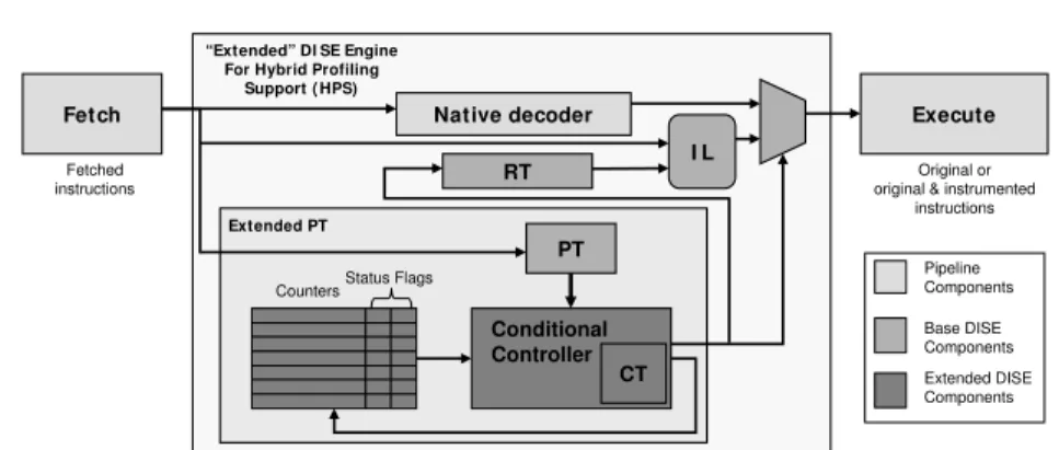
To reduce the number of replacements that DISE performs, we extend DISE with a new functionality calledconditional control. Conditional control, in essence, moves the check of the sampling flag out of the replacement sequence (software) and into the DISE engine (hardware). Conditional control enables HPS to instrument profiled instructions only while the sampling flag is set. To enable conditional control, we modify the DISE engine and production specification.
Figure 4 shows the DISE extensions that enable our efficient implementation of HPS. Instead of requiring that pattern specifications in the DISE ACF be imple-mented using unconditional matches, we allowconditional pattern specification. We add a masking layer which implements conditional matching based on the status flags of internal counters (we currently consider only overflow and zero status flags). HPS manages internal counters using micro-instructions that are defined as part of the DISE productions. HPS stores these microinstructions in an associative table that we have defined called the Conditionals Table (CT). The CT is similar in structure (but smaller in size) to the pattern table (PT) defined as part of the original DISE infrastructure. The RT is part of the original DISE implementation and holds the replacement instruction sequences.
We define a set of lightweight micro-instructions to manage the internal counters and extend the pattern specification language to allow for checking of the status bits. The operations include only those that can be implemented with simple logic
Fetch Native decoder Execute
Extended PT
RT I L
“Extended” DI SE Engine For Hybrid Profiling
Support (HPS)
PT Fetched
instructions original & instrumentedOriginal or
instructions
CountersStatus Flags
Conditional Controller CT Pipeline Components Base DISE Components Extended DISE Components
Fig. 4. HPS extensions to DISE. HPS moves conditional control of instrumentation out of the critical path and into a dedicated controller.
Extended DISE Production Specifications DISE_Production :=PatternÁReplacement , Conditional_Control Pattern :=Instruction_Pattern && Conditional
Instruction_Pattern :=[Original DISE Pattern Specifications]
Conditional :=( [ ! ] (overflow_N | zero_N )) [ (|| |&&) Conditional ] Replacement :=null|[Original DISE Replacement Specifications]
Conditional_Control :=(null |inc_N|dec_N|set_N(dise_reg)) [ ,Conditional_Control]
Fig. 5. HPS pattern and replacement specification grammar (extended from the original DISE production specification grammar).
and executed within the cycle bounds of the decode stage. These include increment, decrement, checking of status (zero and overflow) flags, and copying a value from a HPS-internal register to a counter.
Figure 5 shows the extended DISE production specification that enables condi-tional control within a DISE ACF. We extend the root production, (DISE Production) and the Pattern production to implement conditional control. We added Condi-tional Control and CondiCondi-tional productions that allow the ACF writer to specify simple conditional expressions. These expressions check the status flags for a partic-ular counter for overflow and zero. The microinstructions that we defined are inc N and dec N which increment and decrement DISE counter N, respectively (where N varies between 0 and the number of DISE-private counters). The microinstruction set N (dise reg) sets counter N with a value retrieved from the DISE-private reg-ister dise reg. A production can set the Conditional Control section to null if no conditional microinstruction is required.
Although we allow for arbitrary logic expression on the status bits associated with each counter, in actuality, the number of possible logic functions for a finite set of counters is limited to:
(numberOf Counters∗numberOf StatusBits)2
We only consider two status bits: overflow and zero. The number of counters is a design parameter, and can be as small as 2 (e.g., to implement bursty tracing), or some higher number to allow for more elaborate profiling schemes or functionality. HPS designs with a small number of counters can be efficiently implemented using
a simple truth-table stored in a small n×1 memory (n is 16 for our particular design instance). This small lookup table implements the functionality of the CT and allows us to constrain the processing delay to within the cycle bounds of the decode stage. The PT processing delay is also within the single cycle bounds of the decode stage as described in the original DISE architecture [Corliss et al. 2003b]. Another DISE extension that we make for HPS is to enable specification of pat-tern productions without replacement sequences. This change is reflected in the optional Replacement production: null. When HPS encounters a pattern pro-duction rule with a null replacement specification, the pattern match fails upon completion. As a result, HPS simply forwards the current instruction through the decode stage unimpeded, while still permitting local conditional microinstructions. This implementation (match failure upon encountering a null replacement) is key to enabling low overhead in HPS, since the 1-cycle penalty is imposed only when an instruction is replaced.
3.4 Taking Samples
HPS is flexible in that it can implement a number of different, existing or novel, simple or complex, sample triggering strategies. We use HPS for two different types of sample triggers: an external trigger or an internal HPS-managed trigger. External Sampling Triggers
To take periodic or random samples, we can trigger sampling by HPS using an external signal such as a timer or randomly generated interrupt. To do so requires that authorized software be able to set and unset the sampling flag. To enable this, we use a variation of theAware ACF described in [Corliss et al. 2003b]. We define an HPS production that is matched by a special purpose no-op instruction (usually one of the reserved instructions in the instruction set architecture (ISA)). We refer to this instruction as on trig inst. The execution of this special instruction will cause the sampling flag (in this instance the zero status flag of counter number 0) to be turned on.
P0 :T.OP==on trig inst→set0(HP S R0), null (1)
This production specifies the pattern T.OP == trig inst as a successful match.
T.OP is an attribute of the instruction being decoded that identifies the opera-tion code of the instrucopera-tion. On a match, HPS attempts to use the replacement (set 0(HP S R0), null). set 0(HP S R0) is a conditional microinstruction which causes HPS to copy the contents of the DISE-private register HPS-R0 to counter 0. HPS R0 holds the constant 0. Since the replacement also contains null, the production fails and the original instruction executes unimpeded. We can use a dif-ferent special instruction to turn off the sampling flag (in this case the HPS register HPS-R1 holds the value 1:
P0 :T.OP ==of f trig inst→set 0(HP S R1), null (2)
(We can also use the microinstruction inc 0 to increment the counter and implicitly clear the zero flag causing sampling to stop).
Profile consumers make use of these status bits as part of their profiling (in-strumentation) productions. For example, if we are interested in profiling method
invocations, we use the following production:
P0 : T.OP CLASS==proc call&&zero0→null, RO R0 : call(HotM ethod Handler);T.IN SN
In the above example, whenever the instruction of interest is encountered (pro-cedure call)and if the zero flag of HPS counter number 0 (also referred to as the sampling flag) is true (on), the replacement sequence R0 is streamed into the exe-cutions stream. R0 is simply a call to the profile handler and the original matched instruction (T.INSN). When the sampling flag is off (i.e. zero 0 is false), the pat-tern of P0 will fail and the original instruction is forwarded through the pipeline unimpeded.
Internal Sampling Triggers
The HPS design also supports the implementation of more complex sampling schemes, such as the sampling framework introduced by Arnold et al. [Arnold and Ryder 2001] and extended in [Hirzel and Chilimbi 2001; Hauswirth and Chilimbi 2004]. The sampling frameworkuses code duplication, instruments one copy with pro-filing instructions and transfers control from the uninstrumented to the instru-mented copy according to a counter and conditional checks. The counter (sampling counter(s)), maintained in the uninstrumented code, is incremented on each loop back edge (backward branch) and method invocation. When it exceeds a given threshold, control is transfered to the instrumented code. While in the instru-mented code, profiling data is collected, usually at the expense of reduced perfor-mance. Control is transfered back to uninstrumented code at the next backward branch or method invocation. The extension to thesampling frameworkis called bursty tracingand allows the system to remain in the instrumented code region for a variable burst length, i.e. multiple passes through the checking boundaries (method invocations and loop backedges). Longer bursts are enabled by inserting burst counters and conditional checks in the instrumented copy. In addition, mul-tiple counters can be used in the uninstrumented code to allow for more complex profiling coverage [Hauswirth and Chilimbi 2004].
We can use HPS to implement the sampling framework without code duplica-tion and without introducing anychecking overhead (the cost of incrementing and checking the sampling flag in the uninstrumented code and of the burst flag in instrumented code - also known as the basic overhead [Arnold and Ryder 2001]). We articulate the details of doing so and the necessary productions that enable this in [Mousa and Krintz 2005]. In summary, we implement the sampling and burst flag manipulation as HPS counters (in hardware). When sampling is turned off and a backward branch or method invocation is encountered, HPS increments the sampling flag counter. When that counter overflows (implicitly setting the overflow flag), sampling commences. When this flag is set and HPS encounters an instruc-tion of interest, HPS replaces the instrucinstruc-tion with the profiling instrumentainstruc-tion as previously described. When sampling is turned on and HPS encounters a back-ward branch or method invocation, HPS increments the burst counter. When the burst counter overflows, HPS resets the sampling and the burst counter to their initial values (turning off the overflow bit of the sampling counter and
terminat-ing the samplterminat-ing session). The initial values of the samplterminat-ing and burst flag is the maximum counter value minus the sampling and burst threshold, respectively.
This HPS implementation of the sampling framework eliminates all basic over-head from the maintenance and checking of sampling and burst counters in software. We evaluate the benefits of using HPS for sample-based profiling in [Mousa and Krintz 2005]. We show that by using HPS we reduce the cost of profiling by up to 19% (average 11%) as compared to software-based sampling techniques [Arnold and Ryder 2001; Hirzel and Chilimbi 2001]. We achieve these reductions while eliminating the need for code duplication and while maintaining the flexibility and ease of use characteristic of a software system.
Furthermore, for any sample triggering strategy, internal or external, HPS im-poses no profiling overhead on the executing program, weather direct or indirect, when the sampling flag is unset (i.e. sampling is turned off). The only source of overhead HPS imposes on program execution is the profiling overhead. Profil-ing overhead is the cost of executProfil-ing additional instructions for profile collection. The amount of profile overhead imposed by HPS depends on the duration of the sampling period and the profile type. The profile type dictates which instructions are inserted into the code and the points at which this code is inserted. We next describe how to specify productions for different profile types.
3.5 Specifying Profile Types in HPS
HPS is flexible in that it can implement any instruction-based profiling technique by specifying an ACF for each profile type. We use HPS to implement three different profile types: hot code region, hot call pair, and hot method. These profile types are widely used in dynamic and adaptive optimization systems [Arnold et al. 2000; Cierniak et al. 2000; SunHotSpot ].
Code regions are profiles that estimate basic block behavior and are generally efficient to collect. Each event in the profile is a dynamic branch; the data value for which is the cumulative number of instructions since the previous dynamic branch. Method profiles estimate the time spent in a method; for each method, we record the number of invocations as well as the number of backward branches taken. Call pair profiles are invocation counts for each caller-callee pair executed. We use the term “hot” to indicate that we are interested in the events with the highest values (i.e. that are most frequently occurring).
We show the HPS productions for each of these profile types in Figure 6. As before, P identifies a pattern production and R identifies a replacement production. These ACFs execute no conditional microinstructions. They do employ conditional replacement however – only when the zero status register of HPS internal counter 0 is set, will HPS replace a matched instruction. These productions are controlled by the external trigger sampling strategy described above.
Currently we insert a call to the profile collection routine for each profile type. The typical size of a profile handler is a few hundred bytes. As such, several profile types can be implemented at once. We consider only a single profile type at a time in our evaluation of HPS. The only additional change required to enable collection of multiple profile types at once is to have multiple profile productions active simultaneously while merging the pattern specifications and replacement sequences of overlapping profiles.
Profile Type Productions Hot Code Region Analysis
P1:T.OPCLASS == branch && zero_0 ÁR1, null R1:call(Branch_handler,T.INSN);
T.INSN; Hot Method Analysis
P2:T.OPCLASS == proc_call || (T.OPCLASS ==branch && T.PC < T.Target) && zero_0 ÁR2, null R2:call(HotMethod_handler,T.INSN);
T.INSN; Hot Call Pair Analysis
P3:T.OPCLASS == proc_call && zero_0 ÁR3, null R3:call(CallPair_handler,T.INSN);
T.INSN;
Fig. 6. Pattern and replacement productions for the three different profile types that we investi-gated for remote performance profiling of deployed, embedded device software: hot code region, hot method, and hot call pair profiling.
In the next section, we detail how we set the HPS sampling flag (i.e. apply an external trigger). Specifically, we use intelligent, phase-based, selection of profiling points to guide HPS sample toggling. When the phase-aware sampler designates a program execution interval to sample, it sets the HPS sampling flag (moves 0 into HPS counter number 0 to set the counter’s zero status). The sampler unsets the counter at the end of the interval – thus imposing no overhead on the execution of unsampled intervals.
4. PHASE-AWARE SAMPLING
Figure 7 depicts our implementation of Phase-Aware Profiling. The system con-siders individual, fixed-length periods of program execution at at time. We use an interval length of 10 million instructions in this paper. To predict the phase in which a future interval will be, we employ the Phase Tracker hardware that we proposed in prior work [Sherwood et al. 2003]. The Phase Tracker is a small, low area, low overhead hardware resource that consumes approximately 4 picojoules of energy per dynamic branch (this means that on a high speed machine that executes 1 branch every 2ns, it will consume around 2 mW). The Phase Tracker (figure 7:A) collects the dynamic branch behavior of a program into intervals and segregates the intervals into phases according to a similarity threshold computed from the interval execution characteristics.
The Phase Tracker uses a similarity threshold to govern the number of phases generated from the set of intervals executed by the program. A higher threshold value will generate fewer phases, each consisting of more intervals, but with a higher similarity variance across the intervals of any single phase. The threshold can therefore be adjusted according to the desired sampling rate, and the resulting profile will represent the most diverse and relevant sets of dynamic behavior.
The Phase Tracker uses the program counter value of branch instructions, along with the number of executed instructions between branches, to produce a prediction for the phase of the next interval (the complete details on the prediction process can be found in [Sherwood et al. 2003]). Prior work has shown the accuracy of the Phase Tracker phase prediction to be 85-90% [Sherwood et al. 2003]. We assume a prediction accuracy of 100% in this work; as such, our results indicate an upper bound on the potential of phase-aware profiling performance. [Pereira et al. 2005]
Phase Tracker
ID Sam ple? Count
# inst PC P h as e ID Wireless Network Interface A B E Hybrid Profiling Support (HPS) OS Code C Profile Buffer P h as e T ra ce D
Fig. 7. Overview of the phase-aware profiling scheme. Phases are tracked in hardware (A) and the results are fed to a small table that tracks the state of each phase (B). When a phase is deemed to be important, the profiler (HPS) is notified and a sample is taken (C). The sample is stored in a small profile buffer (D). This information is then transmitted back to a trace aggregation center (E).
use a similar methodology to our phase-aware sampling system to significantly re-duce the overhead of cycle-accurate architectural simulation. The phase tracker in this work identifies and simulates intervals that represent unique (per-phase) execu-tion behaviors. This prior work does not assume perfect Phase Tracker predicexecu-tion and achieves a 3.2% error in cycle count on average over exhaustive simulation.
Since the Phase Tracker is in hardware, it monitors the entire system, i.e. it is shared by multiple processes (much like hardware performance monitors (HPMs)). In our system we use the Phase Tracker to monitor a single process at a time. To distinguish per-process phase data, the operating system toggles phase tracking, via a register in the Phase Tracker hardware, upon a context switch. We only consider single-process phase tracking in this work; we plan to consider concurrent phase tracking as part of future work.
The Phase Tracker outputs a phase ID, which is a unique identifier for the be-havior likely to be observed in the next interval. We store the phase IDs in a small table which tracks each phase and identifies when a sample should be taken. We have found that a fully associative table of size 20 is sufficient to minimize the num-ber of misses using random replacement. In general, the worst case is one in which two similar behaviors are sampled more than once as a result of a table miss. The performance effects from such misses, however, are negligible for tables of this size. The table tracks a list of phase IDs and stores a “sampled bit” that indicates if the phase has already been sampled. Additionally, we record a count of the number of times this phase has been seen in the past.
When the Phase Tracker predicts that the next interval is one from a previously unseen phase, it signals a lightweight profiling daemon (background thread). The daemon tracks the number of intervals encountered for newly executed phases and selects the most appropriate one for sampling.
Ideally, the most representative interval - i.e. most similar to the phase’s other intervals - should be selected for profiling. Doing so online, however, is a challenge because we are not aware of the occurrence of future phase intervals. Therefore, we use a heuristic that quickly identifies a representative interval so that we do not miss the profiling of important phases. In our evaluation section, we consider using one of the first initial intervals encountered for a new phase and compare this
pol-icy to oracle-based approaches (centroid and random) that use future knowledge to identify the best representative interval of a phase. In general, we find that the first interval encountered is not a good representative since it commonly contains exe-cution behaviors from the previous phase or a phase transition. The third interval is commonly sufficient to avoid this “warm-up” period.
Once the daemon identifies an interval to sample, it executes a special profile-toggling instruction. This instruction is equivalent to a no-op (it performs no work and imposes a single cycle pipeline performance penalty). Only authorized agents (processes that are granted such permission by the Operating System, e.g. the profiling daemon) may execute this instruction. Consuming this instruction causes HPS to set the sampling flag (figure 7:C). This is the external trigger scenario described in section 3.4. This simple mechanism is implemented using a single HPS-private counter and requires a single instruction to turn profiling on and off.
When HPS encounters this instruction during the decode stage of the pipeline, it will match it against the pattern in production P0 from Equation 1. This pat-tern causes HPS to execute the microinstructionset 0specified in the conditional control section of P0. This will set the zero status flag in HPS-private counter 0. This status bit acts as the HPS sampling flag. When HPS encounters the next instruction of interest (event to be sampled), it replaces the instruction with the call to the profiling event handler as defined by the productions in figure 6. HPS does so dynamically for each instruction of interest until the sampling flag is turned off. At which time HPS simply forwards the instructions of interest through the pipeline unimpeded. The instructions of interest are those for which there are pro-filing production sequences such as those described in section 3.5 for the external toggle HPS scenario.
Once the profile has been generated, the profile daemon stores it in a specialized profile buffer and tags the profile with the phase identifier (figure 7:D). In addition to the profile data, the daemon records a trace of phase IDs from intervals in previously seen phases. This enables us to reconstruct accurate a time-varying behavior of the program if necessary.
Once the buffer fills, we must empty it via network transmission. At this point, the profile daemon transfers the profile over a wireless network back to some data center for further study and analysis (figure 7:E). In our embedded system study (section 5.4), we evaluate the efficacy of transferring data intermittently while the program is executing (e.g. when storage is limited) as well as transferring the com-plete phase trace once the program terminates. Since communication consumes significant battery power in mobile devices, we must ensure that we minimize the number of bytes transfered. As such, in addition to using phase behavior to reduce profile size, we also incorporate compression of the trace prior to transmission. However, the application of compression consumes computational resources. We include the effect of this tradeoff (increased computation for decreased communi-cation due to compression) as part of the empirical evaluation of our approach. In general, we found that the benefit of compression due to the reduced communica-tion overhead far outweighs the computacommunica-tional overhead we introduce in terms of battery power.
5. EMPIRICAL EVALUATION
In this section, we evaluate the efficacy of our remote profiling system. We first overview our empirical methodology. We then present an evaluation of our DISE extensions that enable HPS (subsection 5.2), and of the accuracy and overhead of our system (subsection 5.3) using a general-purpose benchmark suite and processor. In subsection 5.4 we evaluate our system in the context of a resource-constrained device, its applications, and its power consumption.
5.1 Methodology
We employ a cycle-accurate simulation platform and simulator parameterization identical to that used in the original DISE studies [Corliss et al. 2002; 2003a; 2003b; 2005]. The platform is an extension to SimpleScalar [Burger and Austin 1997] for the Alpha processor instruction set and system call definitions.
Our simulation environment models a 4-way superscalar MIPS R10000-like pro-cessor. It simulates a 12 stage pipeline with 128 entry reorder buffers and 80 reservation stations. Aggressive branch and load speculation is performed and an on-chip memory with 32KB instruction and data caches and a unified 1MB L2 cache is modeled. The DISE mechanism (and HPS system) is configured with 32 PT entries and 2K RT entries each occupying 8 bytes. We also modified the simu-lator to emulate the capture of phase information as described in [Sherwood et al. 2003] with an interval size of 10 million instructions. We extend the DISE simu-lation engine to export the semantics of the conditional controls that we define in section 3.
To generate the instructions for profile collection using each of our three profile types (section 3.5), we write the code using the C language and compile it for our target platform (Alpha EV6). We hand-optimize the generated assembly to ensure compactness. We also insert a no-op instruction to simulate the single cycle stall associated with each replacement. The no-op instruction produces the desired result since the stall due to DISE replacements only affects the decode stage (i.e. delays the propagation of the single instruction that is macro-replaced) and does not impact the later pipeline stages.
We evaluate the performance and profile quality of our system using the bench-marks of the SPECINT2000. We compile the benchbench-marks for the Alpha EV6 platform using GCC 3.2.2 with the -O4 optimization flag. We report results for complete runs on the train input set. We considered other inputs and found the trends in our data to be the same as that we present herein.
Figure 8 shows some of the dynamic behavior metrics for the SPECINT2000 benchmarks used in our empirical studies. Method count is the number of unique methods in the benchmark whileCall sites is the number of static call operations. Call Pairs is the number of unique call site and target address pairing observed in the dynamic execution of the benchmark. The extra number of call pairs beyond the number of call sites indicates a number of indirect jumps. Call count is the number of dynamic calls made during the benchmark’s execution. Dynamic Branch Count and Dynamic Instructions is the the number of branches and instructions executed, respectively. These dynamic metrics are relevant to the performance profiles we investigate: hot code region (branches), hot method, and hot call pair
method
Count SitesCall PairsCall Call Count(millions)
Dynamic Branch Cnt (millions) Dynamic Instructions (millions) bzip2 106 245 245 44.6 1,006 4,546 crafty 165 792 792 43.4 496 2,542 eon.cook 600 2,032 2,068 36.9 198 1,720 eon.kajiya 603 2,039 2,076 183.3 998 8,564 eon.rushmeier 603 2,049 2,086 54.3 296 2,497 gap 487 1,779 2,672 18.8 167 723 gcc 1,234 7,565 7,671 22.1 317 1,199 gzip 113 218 218 25.5 351 1,531 mcf 118 218 218 238.2 2,040 8,829 parser 338 1,149 1,151 82.0 690 2,798 twolf 238 1,120 1,120 104.3 1,663 12,442 vpr.place 180 627 627 13.9 169 1,466 vpr.route 264 1,055 1,055 84.5 1,152 10,238 Average 388 1,607 1,692 73 734 4,546 Fig. 8. Select Benchmark statistics relevant to the profiles collected. profiles.
5.2 HPS Performance
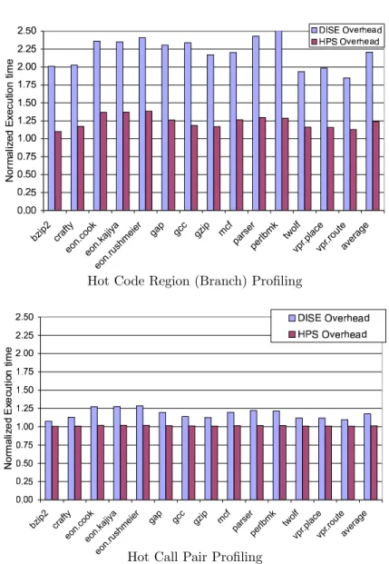
We first evaluate the performance impact of our HPS extensions that enable condi-tional control within the DISE engine. Figure 9 shows the overhead of sample-based hot code region (top graph) and hot call pair (bottom graph) profiling using DISE without conditional controls (left bar) and with our HPS optimizations (right bar). Each bar is the execution time for each program normalized to execution without DISE and without profiling. For this data, we use periodic sampling at a frequency of 1/100 events.
The data shows that HPS (i.e. DISE with conditional controls) significantly re-duces the overhead of a naive, DISE sampling strategy. The overhead that HPS introduces is profiling overhead alone – the cost of executing the extra instrumen-tation instructions for each event of interest. The DISE data includes this overhead as well as the basic overhead for manipulating the sampling flag and the cost of checking that flag as part of the unconditional replacement sequences.
On average, DISE sampling introduces a 120% increase in execution time for hot code region (branch) profiling, while HPS only introduces a 24% increase. For hot call pair profiling the overhead of DISE sampling is 18%, while HPS’s overhead is only 1.3%. Hot method profiling exhibits performance characteristics that are similar to hot call pair profiling. As such, we omit this data for brevity.
5.3 Phase-Aware Sampling
To evaluate the impact of remote profiling, we examine its accuracy versus its overhead using four different profile collection strategies:
—Exhaustive - gather an exact profile for each interval. We use this strategy to evaluate the accuracy of the other policies.
Hot Code Region (Branch) Profiling
Hot Call Pair Profiling
Fig. 9. DISE vs HPS for performance sampling: The overhead introduced by each of the individual profile types. The DISE data is the overhead of sampling without our HPS extensions (i.e. moving sampling flag manipulation and checking into the DISE engine). The right bar is the overhead introduced by HPS (i.e only the profiling overhead). The top graph is the overhead for profiling code regions (an estimation of basic block behavior). The bottom graph is the overhead for profiling call pairs. We omit the graph for method profiling for brevity since it is similar to that for call pair profiling. On average DISE introduces 120% overhead for code region profiling and 18% for call pair profiling. HPS introduces 23% and 1.3% overhead, on average, for these profile types respectively.
Fig. 10. Evaluation of representative selection policies. The graph shows the average error in block counts at 1% sample rate for different representative selection schemes. The black bar shows the performance of average random sampling (non-phase-based).
—Random Sampling - gather a profile for interval i with a probability of 1/P for some P
—Phase-based - gather a profile for every interval that is dissimilar from all previ-ously gathered intervals, given some threshold of similarity.
For the periodic and random strategies, we gather data for different sampling frequencies. The number of intervals we profile, and therefore the percentage of total execution that we profile, depends on the sampling period N. We perform experiments for a range of sampling frequencies which correspond to a range of overheads and accuracies. Because a truly random strategy is at the whim of chance as to whether or not it performs well, we characterize two aspects of random profiling for each of the different percent-sampled values: 1) we compute the average error across 10 runs (avg random), and 2) we compute the maximum error seen across 10 runs (max random). To get a range of accuracies and overheads, we adjust the parameter P and examine the effect.
For phase-aware profiling, as we have described previously, we begin with an implementation of the phase prediction system that we have developed in prior work [Sherwood et al. 2003]. We identify empirically, the best interval from each phase to act as the representative from that phase. Figure 10 shows the percentage error at 1% sampled for four different representative selection policies for phase-based profiling. The y axis shows percentage error in basic block counts. The different polices for representative selection that we evaluate are (a)first: select the first interval as the representative, (b) centroid: select the centroid of the intervals in the phase as the representative, (c) third: select the third interval as the representative. (d)random: randomly select one representative from all intervals in the phase (we report performance for this strategy as the average performance of 5 selections). For comparison, we also show the error that the random sampling strategy, that we describe above, produces. This strategy chooses random samples from the entire program (black bar on far right).
0 5 10 15 20 25 % Program Sampled 0 5 10 15 20
% Error in Code Region Profile
avg random max random periodic phaseaware
Fig. 11. Average error in code region profile for various sampling percentages.
As expected, the centroid method,centroid, performs the best: its error remains low even when we sample very little of the program. First and random perform the worst. This happens since the first is not representative of the steady state (the phase is just warming up) and because selecting randomly can result in selection of a representative that is dissimilar to all others. Third enables accuracy that is between that ofbestandfirst/random. That is,thirdis able to select an interval that is more representative of the steady state of the phase thanfirstandrandom. Moreover, third is simple and can be implemented without additional overhead. As such, we usethirdfor the rest of the results in the paper.
Unlike the random and periodic sampling approaches, there is no sampling fre-quency variable that we can vary to get different tradeoff points between accuracy and overhead. Instead, we achieve a similar effect by dynamically tuning the simi-larity threshold. The similarity threshold determines the cutoff point at which two intervals are said to be similar and hence are part of the same phase. As we lower the threshold, the system detects more unique phases, each with a fewer number of intervals. As this occurs, the system takes more samples (since there are more unique phases). This both increases the percentage of the program’s execution that the system samples and improves the accuracy of the resulting profile.
Profile Accuracy vs Overhead
To measure profile accuracy, we compare each sampled profile to the exhaustive profile. We compute the percentage error in the code region profiles as our accuracy metric. The code region profiles contain counts for each dynamic branch. We compute the element-wise difference in branch counts between a sampled profile and the exhaustive profile. We then divide this value by the total counts in the exhaustive profile to produce the error percentage. The best sampling strategy is the one that produces the least amount of error for the smallest percentage of the program that is sampled.
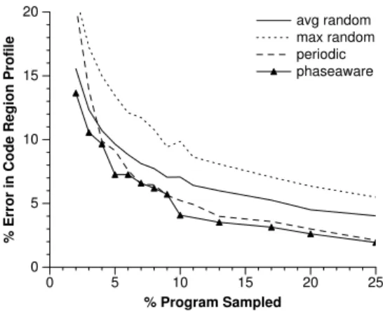
Figure 11 shows the average error across benchmarks using the third interval of each phase as the phase representative. The graph compares the accuracy of each of the different sampling strategies,avg random,max random,periodic, and phase-aware. The y-axis is the error percentage in total branch counts (not just
the hot branches which we study later) and the x-axis is the percentage of the program that was sampled for a given parameterization of each strategy.
The data indicates that on average, phase-aware profiling achieves lower error for small percent-sampled values than the other strategies. The error for periodic sampling approaches that of phase-aware sampling for some percentages sampled – both approaches require 10% of the program to be sampled to achieve 5% or less error. The random strategy requires that 20% of the program be sampled to achieve an error of less than 5%. For lower percent sampled values, the benefits from our system increase substantially.
We next demonstrate that phase-aware sampling is not restricted to any single profile type by showing that it performs well for others. We evaluate the efficacy of each of the sampling strategies in identifying frequently executing parts of the program. Profiles that capture frequently executing parts are commonly used for feedback directed optimization, e.g., hot code regions, hot methods, and hot call-pairs, and as such are important profile types for our distributed optimization system. We measure the error produced by each of the profiling strategies for these profile types. We define “hot” as the top 15% of the most frequently executed events.
Figure 12 shows the results. The x axis is the percent of the program that was sampled, and the y axis is the percentage error in identifying hot branches, hot call-pairs and hot methods, on average across benchmarks. We omit max random and average random data from the hot call pair graph since both were in a range significantly larger than the other strategies. Average random ranges from 33-53% error and max random ranges from 49-64% error.
The graphs show that the phase-aware strategy performs considerably better than both random and periodic sampling for all three profile types. Assuming an error of 5%, the phase aware strategy needs only to sample 5% for hot methods and hot branches, and 20% for hot call pairs. Periodic sampling performs similarly to phase-aware sampling for call pairs, but requires that we sample 10% of the program for hot methods and 20% of the program for hot branches. Random sampling rarely achieves an error of 5% or less; however, it does so for hot methods for which it requires that we sample 20% of the program.
In Figure 13, we quantify these overhead percentages (assuming 5% error) for individual benchmarks using three tables. The top table is for hot code region (dynamic branch) profiling, the middle table is for hot method profiling, and the bottom table is for hot call-pairs. We chose 5% error as our cutoff arbitrarily; however, we selected a value that we believe to be tolerable and amortized by commonly used, profile-based, dynamic optimizations. For lower error values, the benefits of our system increase significantly since phase aware profiling is able to extract unique and important program behaviors by sampling only a very small portion of the execution.
Each table reports data for the three profiling strategies: phase-based, periodic, and (averaged) random sampling. For average random, if the error does not reach 5% or less, we use a percent sampled value of 25%. The data in columns two, three, and five show profiling overhead in millions of cycles for each of the benchmarks. Columns four and six show the percent reduction in this overhead due to phase-aware sampling.
0 5 10 15 20 25 % Program Sampled 0 5 10 15 20 25
% Error in Code Region Hotness
avg random max random periodic phaseaware
(1) Hot Code Region Profiling
0 5 10 15 20 25 % Program Sampled 0 5 10 15 20 25
% Error in Method Hotness
avg random max random periodic phaseaware 0 5 10 15 20 25 % Program Sampled 0 5 10 15 20 25
% Error in Callpair Hotness
periodic phaseaware
(2) Hot Method Profiling (3) Hot Call-pair Profiling Fig. 12. Efficacy of different sampling strategies for different profile types. We omit max random and average random data from the hot call pair graph since both were in a range significantly larger than the other strategies. Average random ranges from 33-53% error and max random ranges from 49-64% error.
The final row in each table shows the average across benchmarks. For hot code re-gions, phase-aware profiling reduces the overhead of periodic and random sampling by 76% and 80%, respectively, on average. This reduction is 50% and 76%, respec-tively, for hot methods. The primary reasons for these benefits are two-fold: (1) Random and periodic sampling collect redundant information (i.e. profiles of the execution that they have already collected); and (2) random and periodic sampling techniques miss important behaviors (which degrades accuracy) which phase-aware sampling is able to capture.
For hot call pairs, phase-aware sampling reduces the overhead of random sam-pling by 22% on average. However, as visible in the graphs in Figure 12, phase and periodic sampling perform similarly for this profile type. For some benchmarks, periodic sampling for hot call pairs outperforms phase-based sampling. One reason for this is that the absolute number of hot call pairs is very small for most bench-marks. As a result, one or two missed pairs can result in a significant increase in percentage error. This is the case for bzip2.
(1) Hot Code Region Profiling
(2) Hot Method Profiling
(3) Hot Call Pair Profiling
Fig. 13. Overhead of different sampling strategies for different profile types, assum-ing a 5% error rate. The data in columns 2, 3, and 5 is the profilassum-ing overhead in millions of cycles. Columns 4 and 6 show the percent reduction in this overhead due to phase-aware sampling.
Dynamic Statistics Average Instr / s Static Branches Instructions Cache Energy Time Instr Type Joules / s (Millions) Benchmark Branches (Millions) (Millions) Miss Rate (Joules) (seconds) IREG 0.865 204.790 gsmdecode 572 182.05 1610.05 0.000 29.93 16.35 IMEM-R 0.973 19.462 gsmencode 748 79.42 2562.29 0.000 29.38 19.93 IMEM-Rcache 0.000 137.510 jpegdecode 930 111.76 1421.33 0.006 46.50 21.87 IMEM-W 1.340 11.625 jpegencode 1175 433.70 4218.60 0.002 100.65 51.41 FPREG 0.965 0.439 mpegdecode 1104 309.95 3007.85 0.001 65.03 900.63
mpegencode 2216 244.25 4196.19 0.001 52.63 282.40 Wireless Specification Max Average 1124 226.86 2836.05 0.002 54.02 215.43 Card 5V*0.285A Bandwidth
Transmit 1.425 11Mb/s
(a) (b)
Fig. 14. StrongARM methodology. (a) shows the general MediaBench benchmark statistics. (b) shows the empirical data that we use to estimate energy consumption. The second column is Joules per second and the final column is instructions per second for the instruction types and bandwidth for wireless transmission.
5.4 Phase-Aware Remote Profiling for Embedded Devices
To investigate the efficacy of phase-aware remote profiling for embedded devices, we also evaluate our approach for a popular hand-held device processor, the Intel StrongARM. We employ SimpleScalar to emulate a StrongARM processor. As in the prior section, we modify the simulator to emulate the capture of phase infor-mation as described in [Sherwood et al. 2003] with an interval size of 10 million instructions. The authors in [Lau et al. 2005] explore the overhead/accuracy trade-offs and efficacy of using variable sized intervals. Our large, fixed-size intervals are practical for resource constrained systems since they minimize sample storage and maintenance overhead and simplify phase prediction. Since we are interested in the efficacy of remote profiling for mobile devices, we estimate the overhead of our system in terms of power consumption.
We evaluate our system using six benchmarks from the MediaBench benchmark suite [Lee et al. 1997], a suite designed for the empirical evaluation of media ap-plications. The benchmarks we use include encoding and decoding programs for mpeg (movie), jpeg (picture), and gsm (voice). We show the basic statistics for the programs and the inputs we used in this study in table (a) of Figure 14. The second column in the table is the number of static branches in the program, which correlates with the size of the branch profiles generated. The next five columns show the dynamic statistics: number of branches executed (in millions), number of instructions executed (in millions), the cache miss rate assuming a 64K, 4-way set associative, instruction and data cache, the energy consumed by executing the program (in Joules), and the execution time (in seconds). Since the inputs that are provided with MediaBench are very short, and because these applications are typically used in a streaming fashion, it was necessary to find more substantial inputs to analyze the realistic long term effects of profiling. We plan to make these inputs available via our web page.
To compute energy consumption and execution time, we use a model that we generate from an actual hardware system. We compute the energy (Joules per second) consumed instruction (including events such as cache misses), per-byte-transmitted energy consumed, and instructions per second. We summarize the values in table (b) of Figure 14. We generate these values using an HP iPAQ H3835