Institute for Advanced Development Studies
Development Research Working Paper Series
No. 10/2006
Welfare Gains from Optimal Policies
in a Partially Dollarized Economy
by:
Carlos Gustavo Machicado
September 2006
The views expressed in the Development Research Working Paper Series are those of the authors and do not necessarily reflect those of the Institute for Advanced Development Studies. Copyrights belong to the authors. Papers may be downloaded for personal use only.
Welfare Gains from Optimal Policies in a
Partially Dollarized Economy
∗
Carlos Gustavo Machicado S.
†September 28, 2006
Abstract
This paper evaluates welfare under optimal monetary andfiscal pol-icy in a dynamic stochastic model of currency substitution and capital. It shows that in a partially dollarized economy, the main optimal policy results, i.e. the Friedman Rule and the zero capital tax, hold. Welfare im-plications of these optimal policies are computed for the Bolivian economy using a second-order approximation technique. The primary conclusions are that the welfare gains under optimal monetary policy are negligible. The welfare gains when optimal fiscal policy is considered alone or in conjunction with optimal monetary policy are sizable and come from the increase in real variables and also by the increase in real balances in local currency. Thus, welfare gains are negatively related to dollarization.
Keywords: Dollarization, Optimal Fiscal and Monetary Policy, Second-order approximation technique.
JEL classification: F31, E61, E63.
∗This paper corresponds to the third chapter of my Phd thesis "Essays on Partially
Dol-larized Economies". I appreciate the help and comments from Romulo Chumacero and Todd Keister.
†Researcher, Institute for Advanced Development Studies, La Paz, Bolivia. E-mail address:
1
Introduction
We already know a fair amount about optimalfiscal and monetary policy for a single-currency economy, but some countries face, for various reasons partial dollarization. Are the optimal policy lessons related to taxes and nominal in-terest rates also valid for this type of economies? This is an important question that I answer in a dynamic stochastic model of currency substitution and capi-tal. I stress the word capital, since most of the papers do not introduce capital when they are analyzing optimal monetary policy. Kydland and Prescott [16] emphasized investment dynamics as an important channel for the transmission of aggregate disturbances, so it is natural to believe capital accumulation should play a role in shaping optimalfiscal and monetary policies.1
Other important issues that have not been analyzed much are the wel-fare implications related to performing optimal policies in partially dollarized economies. It is clear that policies that are optimal or near their optimal level will be welfare improving, but how large or small these welfare gains could be in a partially dollarized economy is a question that has not been answered yet. Compared with the existing literature, this paper shows that the welfare gains are small under optimal monetary policy, but are sizable under optimal fiscal policy. These gains are primarily driven by real balances in local currency.
The welfare gains of shifting from current policies to the optimal policy, refer to the fraction of consumption from the benchmark or current regime that a household would be willing to receive to be compensated for being in that regime and not in the optimal policy regime. I compute the welfare gains associated with optimal policies using the second-order approximation technique developed by Schmitt Grohé and Uribe [24].
Welfare gains based on an evaluation of the utility function have not previ-ously been computed for partially dollarized economies, this is thefirst time that such comparisons are performed. Cavalcanti and Villamil [3] consider currency substitution in a monetary model with transactions technology, and compute welfare gains associated with optimal monetary policies; but, they choose a standard calibration using the U.S. economy as a baseline. Clearly there are big differences between an economy where two monies are used in transactions and the U.S. economy, which is a single currency country.
The papers closer to this work are those of Cavalcanti and Villamil [3] men-tioned above, and Vegh [28], but they only use monetary models with transac-tions technology. This paper contributes to the dollarization literature by using a two-monies-in-the-utility-function model (2MIUF model) to handle monetary andfiscal policy issues. Cavalcanti and Villamil [3] introduce currency substitu-tion as a market distorsubstitu-tion similar to the existence of an informal sector, where markets are incomplete. Here, I introduce dollarization to the model as a shock to the economy. Dollars circulate in the economy and are part of the aggregate demand. The results show that there are some differences in welfare, whenThe one is considering two monies in the utility function.2
1Schmitt Grohé and Uribe ([25]) note also this notable simplification.
Recent research about optimalfiscal and monetary policy has concentrated on introducing nominal rigidities and imperfect competition to this type of mod-els.3 My model constitutes a revisit to the beginning of this literature, because
all the recent models share a characteristic, they do not have capital accumu-lation. It is important to introduce it, especially if we want to see the welfare effects offiscal policies under distortionary taxes on capital income.
The building blocks of my model come from the literature of optimal fiscal and monetary policies, which is a mixture of the publicfinance and the general equilibrium traditions. In this manner, I characterize optimal allocations as solutions of a simple programming problem (the Ramsey problem) and I am particularly interested in the solutions and the associated policies which are called the Ramsey allocations. This is done in the theoretical part of the model. In the empirical part, I do not compute the model with Ramsey policies, instead I assume a benchmark economy and see what happens if this economy shifts to optimal policies. I am interested specially in seeing the magnitudes of the welfare gains associated with these policies.
The foremost theoretical result is that the two major results related to op-timal policies, i.e, the Friedman Rule and the zero tax on capital income hold also for partially dollarized economies without modifications. As Chari,et. al.
[8], assuming homotheticity in the utility function, I show that the optimality of the Friedman Rule holds. This is not a necessary assumption, as it is shown in the numerical example.4
The principal finding, as it relates to fiscal policy, has been that capital taxes should be zero if a steady-state Ramsey allocation exists (see Chamley [5]). Certainly, this is a steady-state result, and in the theoretical section, it is proved in that context. But Chari and Kehoe [4] show that keeping capital income tax rates close to zero after period 1 is also optimal. In the numerical simulations, I show that the same is true for a partially dollarized economy, since all real variables are improved by setting income capital tax to zero. Furthermore the level of dollarization is reduced.
I have calibrated the model for the Bolivian economy, which is a partially dollarized economy. I assume that the monetary policy is implemented by a simple policy rule -the Taylor Rule- where the Monetary Authority sets a target for the inflation rate. Thefiscal policy is implemented through constant capital and labor income taxes.
Welfare gains in terms of permanent consumption associated with optimal policies are computed using a second-order approximation to the policy func-tion. The mainfinding is that by setting the capital tax to zero, the Bolivian economy experiments an important welfare gain of 3.65 percent of permanent consumption. Welfare gains related to optimal fiscal policy have never been computed for a partially dollarized economy, but for example Chari, et.al.[7]
Winkelried [2] and Mendoza [20].
3See Schmitt-Grohe and Uribe [22] and [23], Correiaet. al. [11], and Correia and Teles [10].
4Cavalcanti and Villamil[3]find that the Friedman Rule is not the optimal monetary policy when the transactions cost function is homogeneous of degree one or greater.
find gains of 1.6 percent for a model with high risk aversion and 6.1 percent for an economy with high initial debt. Here, welfare gains come from the fact that consumption, leisure and especially real balances in local money increase as a consequence of the reduction of the capital tax to zero. All these variables are arguments of the utility function.
Morales [21] states that more understanding is needed on the optimal policies for Central Banks in partially dollarized economies, so I analyze welfare effects associated with a reduction in the yearly inflation target from 5 percent to 2 percent. The welfare gains associated with this policy are in the order of 0.0084 percent. Cooley and Hansen [9] estimate the welfare gains from eliminating moderate inflation and they find that they are in the order of 0.4-0.6 percent. The model shows that money is super neutral, and in this case, the increase in welfare comes solely by the increase of the real balances in local money.
I also compute welfare gains associated with the implementation, at the same time, of both optimalfiscal and monetary policy. The results show that agents obtain welfare gains in the order of 3.66 percent of permanent consumption. In this case it is clearly seen that these gains are mainly driven by the reduction of the capital tax to zero. The real variables in the economy change in the same magnitude as when only optimalfiscal policy was implemented, and so welfare gains are very similar. The impact of reducing the inflation target to 2 percent is negligible.
In the three exercises, I find that there are no differences between welfare gains computed with thefirst-order approximation and the second-order approx-imation technique. This means that volatilities do not have welfare implications in the Bolivian economy. The main parameter in explaining welfare is the share that monies have in the utility function. Therefore, I perform a sensitivity analysis with this parameter andfind a negative relation between dollarization and welfare gains. As dollarization increases, the welfare gains decrease, and this relation is more pronounced iffiscal policy is being considered.
The remainder of the paper is organized infive sections. Section 2 describes the structure of the model. Section 3 presents the Ramsey problem and the pri-mal approach to solve it. In section 4, the main theoretical results are provided and proved. Section 5 establishes the calibration of the Bolivian economy and I compute the welfare gains associated to optimal policies using the second-order approximation technique. Finally section 6 offers the concluding remarks.
2
The Model
In this section, I develop a simple dynamic stochastic model of currency substitu-tion and capital. My model is an extension of the monies-in-the-utility-funcsubstitu-tion in a small open economy literature developed by Imrohoroglu [12] and Can-zoneri and Diba [1]. I capture a real world situation where in some countries two monies compete against each other to provide liquidity services. A way to capture this fact is by introducing these two monies (pesos and dollars) in the utility function, where agents have preferences for using both monies. In other
words domestic money and dollars share the same privileges and thus affect utility in the same manner.5
Cavalcanti and Villamil [3] use a model where pesos and dollars enter into a transactions technology. That is another form to introduce partially dollariza-tion into the economy, but more difficult to analyze numerically, so that is why my model is more suitable to analyze policy and welfare implications.
Monies enter in the utility function with a weight (the elasticity of substitu-tion), which will be higher for the foreign currency, if the country is dollarized. Other arguments in the utility function are consumption and leisure. Firms use capital and labor to produce goods and the governmentfinances an exogenous stream of purchases by levying distortionary labor and capital taxes, printing local money, and issuing one-period nominally risk-free bonds.
There is an infinitely lived representative household living in a single-good, stochastic, 2MIUF, economy. Household’s preferences are given by
E0
∞ X
t=0
βtu(ct, mt, dt, lt) (1) where β ∈ (0,1), ct ≥ 0 and lt ≥ 0 denote consumption and leisure at
timetrespectively;u(·)is strictly concave and twice continuously differentiable. Because of the timing in the story underlying the money-in-utility reduced form, I define mt = MPt+1t as the real balances in local currency held in periodt for
periodt+ 1; and dt=εtDt+1
Pt as the real balances in dollars.
6
With one unit of time per period, households divide it between leisureltand labornt.
1 =lt+nt (2)
The single good is produced with capitalktand labornt. The output can be
consumed by households, used by the government, used to augment the capital stock, or used to be traded for dollars in an international market. The economy feasibility constraint is given by:
ct+gt+kt+1+ εtDt+1 Pt − εtDt Pt ≤ AtF(kt, nt) + (1−δ)kt (3) where δ∈(0,1)is the rate at which capital depreciates, gt is an exogenous
sequence of government purchases that will be affected by shocks and where there are also going to be technological shocks At. The production function F(kt, nt)is standard concave and exhibits constant returns to scale.
5As it is typical in a partially dollarized economy, dollars serve as medium of exchange, value reserve and unit of account.
6In a cash-in-hand model we definem
t=MPt
t anddt=
Dt
P∗
t because agents purchase goods within each period.
2.1
Present Value Budget Constraint
The representative household’s period-by-period budget constraint is given by:
ct+ Mt+1 Pt + tDt+1 Pt + Bt+1 Pt +kt+1≤ Mt Pt + (4) tDt Pt + (1 +it) Bt Pt + (1−τkt)rtkt+ (1−τnt)wtnt+ (1−δ)kt
The left-hand side represents the use of funds, and the right-hand side mea-sures the resources at the household’s disposal. It is important to note thatit
is the interest rate on bonds defined the period before; rt is the rental rate of capital;τk
t is the tax on capital income, τnt is the tax on labor income andwt
is the wage rate.
After consolidating two consecutive budget constraints given by equation (1), and defining the real rate of interest as: Rt+1= (1 +it+1)Pt/Pt+1, I arrive
at: ct+Etct+1 Rt+1 +mt it+1 1 +it+1 +Etmt+1 Rt+1 it+2 1 +it+2 +dt µ 1− 1 1 +it+1 εt+1 εt ¶ +Etdt+1 Rt+1 µ 1− 1 1 +it+2 εt+2 εt+1 ¶ ≤ MtP t +εtDt Pt + (1 +it)Bt Pt (5) +(1−τkt)rtkt+ (1−δ)kt+ (1−τnt)wtnt+Et (1−τn t+1)wt+1nt+1 Rt+1
where I have imposed the following no-arbitrage condition to ensure the exis-tence of a competitive equilibrium with bounded budget sets:
Et£(1−τkt+1)rt+1+ 1−δ¤=EtRt+1 (6)
and the no Ponzi-Game conditions:
lim T→∞Et ÃT Y i=0 R−i1 ! MT+1/PT+1 RT+1 = 0; Tlim→∞Et ÃT Y i=0 R−i1 ! DT+1/PT+1 RT+1 = 0; lim T→∞Et à T Y i=0 Ri−1 ! BT+1 PT = 0; Tlim→∞Et ÃT Y i=0 R−i 1 ! kT+1= 0
If condition (6) is violated, the household can make its budget set unbounded by either buying an arbitrarily largekt+1 when the left-hand side is bigger than
the right-hand side, or, in the opposite case, by selling capital short with an arbitrarily large negativekt+1.
By continuing the process of recursively using successive budget constraints and summing over t, we arrive at the household’s present-value budget con-straint: E0 ∞ X t=0 q0t[ct+Itmt+It∗dt−(1−τnt)wtnt]≤ M0 P0 +ε0D0 P0 +(1+i0) B0 P0 +£(1−τk0)r0+ 1−δ¤k0 (7)
whereq0 t = Ãt+1 Y i=0 Ri−1 ! ,It=1+it+1it+1 andIt∗= 1−1+i1t+1 εt+1 εt .
2.2
Firms
In each period, the representativefirm takes(rt, wt)as given and rents capital and labor from households to maximize profits,
max
{kt,nt}
Π=AtF(kt, nt)−rtkt−wtnt
Thefirst order conditions for this problem are:
rt=AtFk(kt, nt) (8)
wt=AtFn(kt, nt) (9)
2.3
Government
The government finances its expenditure stream gt by levying flat-rate
time-varying taxes on earnings from capital at rate τk
t and from labor at rate τnt.
The government might also trade one-period bonds and print domestic money (segniorage). The government’s budget constraint is given by:
gt=τktrtkt+τntwtnt+Bt+1−(1 +it)Bt
Pt +
Mt+1−Mt
Pt (10)
3
The Ramsey Problem
The general approach to characterizing competitive equilibrium with distorting taxes is known in the publicfinance literature as theprimal approachto optimal taxation or to the Ramsey problem. The basic idea is to eliminate all prices and taxes so that the government can be thought of as directly choosing a feasible allocation, subject to constraints that ensure the existence of prices and taxes such that the chosen allocation is consistent with the optimization behavior of households andfirms.
The primal approach, as opposed to the dual approach in which tax rates are viewed as governmental decision, emphasizes the solution of the Ramsey problem. In contrast, the dual approach (see Lucas and Stockey [18]) emphasizes the solution of the household’s problem, more in the style of a typical Real Business Cycle (RBC) model.
3.1
De
fi
nitions
I start this section giving some definitions, which are important for the rest of the paper.
Definition 1 A feasible allocation is a sequence ({kt},{ct},{nt},{dt},{gt} and{At})that satisfies equation (3).
Definition 2 A price system is a 6-tuple of nonnegative bounded sequences ({wt},{rt},{it},{εt},{Rt}and{Pt}).
Definition 3 A 5-tuple of sequences ({gt},©τk t
ª
,{τn
t},{Bt} and {Mt}) rep-resent a government policy.7
Definition 4 A competitive equilibrium is a feasible allocation, a price system, and a government policy such that (a) given the price system and the government policy, the allocation solves both thefirm’s problem and the household’s problem; and (b) given the allocation and the price system, the government policy satisfies the sequence of government budget constraints (10).
There are many competitive equilibrium indexed by different government policies. This multiplicity motivates the Ramsey problem.
Definition 5 Given M0,D0,B0,k0 andP0 the Ramsey Problem is to choose
a competitive equilibrium that maximizes expression (1).
According to the technology constraint (3), capital is reversible and can be transformed back into the consumption good. Thus, the capital stock is afixed factor only one period at a time, soτk
0 is the only tax that we need to restrict
to ensure a closed form solution to the Ramsey problem. These bounds play an important role in shaping the near-term temporal properties of the optimal tax plan, as discussed by Chamley[5] and explored computationally by Jones, Manuelli and Rossi[13].
3.2
The Primal Approach of the Ramsey Problem
For easy exposition, I rewrite equation (7) here.
E0 ∞ X t=0 q0t[ct+Itmt+It∗dt−(1−τnt)wtnt]≤ M0 P0 +ε0D0 P0 +(1+i0) B0 P0 +£(1−τk0)r0+ 1−δ ¤ k0 (11) One advantage of the primal approach is that it is better organized. The basic idea of the primal approach is to recast the issue of choosing optimal taxes and interest rates as a problem of choosing allocations subject to constraints which capture the restrictions on the type of allocations that can be supported as a competitive equilibrium for some choice of taxes and prices.
I develop the Ramsey problem in four steps as in Ljungqvist and Sargent [17].
7M
3.2.1 Constructing the Ramsey plan
Step 1: Letλbe a Lagrange multiplier on the household’s budget constraint (11). Thefirst-order conditions for the households problem are:
ct:βtuc(t)−λq0 t = 0 nt:−βtun(t)−λq0 t[−(1−τnt)wt] = 0 mt:βtum(t)−λq0 tIt= 0 dt:βtud(t)−λq0 tIt∗= 0
from these we obtain
un(t) uc(t) = (1−τ n t)wt (12) um(t) uc(t) =It (13) ud(t) uc(t) =I ∗ t (14)
Profit maximization and factor market equilibrium imply equations (8) and (9).
Step 2: Using equations (12)-(14) we can write equation (11) as:
E0
∞ X
t=0
βt[uc(t)ct+um(t)mt+ud(t)dt−un(t)nt] (15)
≤ uc(0) · M0 P0 +ε0D0 P0 + (1 +i0) B0 P0 +£(1−τk0)r0+ 1−δ ¤ k0 ¸ or E0 ∞ X t=0
βt[uc(t)ct+um(t)mt+ud(t)dt−un(t)nt]−W0= 0 (16)
whereW0is given by:W0(c0, m0, d0, n0) =uc(0)
h M0 P0 + ε0D0 P0 + (1 +i0) B0 P0 + £ (1−τk0)r0+ 1−δ¤k0 i . This equation is called the "implementability constraint". Notice that it is
written with equality. The constraint in the consumer problem is an inequal-ity because of free disposal but under non-satiation, consumers must optimally choose (in CE) to satisfy their budget constraint with equality. Hence in the gov-ernment´s implementability problem, the consumer’s present value constraint must hold with equality.
Looking at (16), people could think that it is optimal for the government to choose a very largeP0to reduceM0/P0to relax the implementability constraint.
Any manipulation of prices at period0would reduce the need for distortionary taxation later on. This is also another way of describing the inflation tax.
To eliminate these possibilities, it can be assumed that all variables in period zero are equal to0.
Step 3: The Ramsey problem consists in maximizing expression (1) subject to equation (16) which is called the implementability constraint and the feasibility constraint (3). The implementability constraint can be thought of as a consumer budget constraint with both the taxes and the prices substituted out by using
first-order conditions.
I assume that the government expenditures are small enough so that the problem has a convex constraint set and so we can use Lagrangian methods.
M axE0 ∞ X t=0 βtu(ct, mt, dt,1−nt) s.t E0 ∞ X t=0 βt[uc(t)ct+um(t)mt+ud(t)dt−un(t)nt]−W0= 0 ct+gt+kt+1+dt−dt−1εtε−t1PPt−t1 ≤AtF(kt, nt) + (1−δ)kt
The Lagrangian is:
J = E0 ∞ X t=0 βt u(ct, mt, dt,1−nt) +Φ · uc(t)ct+um(t)mt+ ud(t)dt−un(t)nt ¸ −θt " ct+gt+kt+1+dt−dt−1εtεt −1 Pt−1 Pt − AtF(kt, nt)−(1−δ)kt # (17) −ΦW0
whereΦandθtare the Lagrange multipliers on the two constraints
respec-tively.
DefineV(ct, mt, dt,1−nt,Φ) = u(ct, mt, dt,1−nt)+Φ[uc(t)ct+um(t)mt+ud(t)dt−un(t)nt], so the Lagrangian is J =E0 ∞ X t=0 βt ( V(ct, mt, dt,1−nt,Φ)−θt " ct+gt+kt+1+dt−dt−1εεt−t1 Pt−1 Pt −AtF(kt, nt)−(1−δ)kt #) −ΦW0 (18) First-order conditions for this problem are:
ct:Vc(t)−θt= 0
nt:−Vn(t)−θt[−AtFn(t)] = 0 mt:Vm(t) = 0
ft:βt[Vd(t)−θt] +βt+1Etθt+1εt+1εt PPt+1t = 0
kt+1:−βtθt+βt+1Etθt+1[At+1Fk(t+ 1) + 1−δ] = 0
These conditions become:
Vn(t) Vc(t)
=AtFn(t) (19)
Vd(t) =Vc(t)−βEtVc(t+ 1) εt+1 εt Pt Pt+1 (21) Vc(t) =βEtVc(t+ 1) [At+1Fk(t+ 1) + 1−δ] (22)
To these we add the feasibility and implementability constraints and seek an allocation{ct, mt, dt, nt, kt}∞t=0 and a multiplier Φthat satisfies the system of difference equations formed by (19)-(??), (3) and (16).
One important difference is introduced in the model because of the inclusion of a second currency in the economy. This can be seen in equation (21). Notice that this equation not only involves real variables, it also involves the inflation rate Pt+1/Pt and the rate of devaluation εt+1/εt. This could impose some
complications in closing the model, but I delay this discussion until section 3.5, where I present the model with functional forms.
Step 4: After an allocation has been found, we obtain the prices from equa-tions (12)-(14).
4
Theoretical Results
In this section, I show that the main theoretical results related to optimalfiscal and monetary policy in a single-currency economy with capital, also apply to this 2MIUF partially dollarized economy. In general, a government facing a partially dollarized economy should follow the same optimal policies as a government in a non-dollarized economy. Dollars and the domestic currency are both neutral and the former are part of the aggregate demand. This could be interpreted as the current account of the economy or as a vintage capital. Perhaps the latter is better as this is a closed economy model.
4.1
The Friedman Rule
The main result related to optimal monetary policy is the so called Friedman Rule.8 This rule states that the optimal policy is to satiate the economy with
real balances by generating a deflation that drives the net nominal interest rate to zero. In a stationary economy, there can be deflation only if the government retires currency with a government surplus (see Ljungqvist and Sargent [17]).
We now ask if such a costly scheme remains optimal when all government revenues must be raised through distortionary taxation in an economy where there are two types of real balances and capital. The answer is yes, and I prove this result as in Chari,et.al.[8], i.e I am going to assume that preferences satisfy homotheticity and separability conditions.
u(ct, mt, dt,1−nt) =U(H(ct, mt, dt),1−nt) (23) 8The optimality of the Friedman Rule is also a characteristic of the "optimum quantity" of money.
whereH is homothetic.
Proposition 1 If the utility function is of the form (23), then the Friedman rule is optimal.
Proof. From step 3 above, we know that Vm(t) = 0 andVc(t) =θt. These
first-order conditions imply:
(1 +Φ) um(t) +Φ[ucm(t)ct+umm(t)mt+udm(t)dt−unm(t)nt] = 0 (1 +Φ) uc(t) +Φ[ucc(t)ct+umc(t)mt+udc(t)dt−unc(t)nt] =θt the assumption of homotheticity (see appendix A for details) allows us to write these two equations as:
Hm[(1 +Φ)UH+Φ(UHHH−UHnn)] = 0 (24)
Hc[(1 +Φ)UH+Φ(UHHH−UHnn)] =θt (25)
Then, dividing (24) by (25) and given thatθt6= 0, we obtain: Hm
Hc = 0 =⇒ um(t)
uc(t) = 0 and then by (13), we haveIt= 0, soit+1= 0.
Clearly, this result comes from the assumption made about preferences, but restrictingH to be homogeneous does not reduce the generality of the result.
Corollary 1 Under the Friedman RuleRt+1=Pt/Pt+1.
Proof. The proof is trivial. It is definedRt+1≡(1 +it+1)PPt+1t as the gross
nominal interest rate. Optimality of the Friedman Rule meansit+1= 0, so the
result is straight forward.
This result is saying that along the optimal path, money and capital yield the same return. It can be seen again thatit+1<0cannot hold in equilibrium.
Ifit+1 were negative, domestic money would yield a higher return than capital
but then the household would not hold any capital. If no one holds capital, however, the return on capital would be infinitely high, which contradicts the assumption that local currency yields a higher return than capital.
Then, the no-arbitrage condition (??) ensures that capital and bonds have the same rate of return. In sum, capital, bonds and money share the same return in the economy.
4.2
Zero Capital Tax
The most important result on optimalfiscal policy is the zero capital tax.9 This is a steady-state result, first proved by Chamley [5] and applied in a variety
9Smoothing of taxes on labor income is also an important result in the literature concerning optimal taxation (see Chari,et.al.[7]).
of circumstances. Sometimes one can establish a much stronger result, namely that optimal capital income taxes are close to zero after only a few periods. Chari and Kehoe [4] show that keeping capital income tax rates close to zero after period 1 is also optimal.
Proposition 2 If there exists a steady-state Ramsey allocation, the associated limiting tax rate on capital is zero.
Proof. Consider the special case in which there is aT ≥0for whichgt=g
for allt≥T. Assume there exists a solution to the Ramsey problem, and that it converges to a time-invariant allocation (steady state). Then from (??) we have
1 =β£AFk+ 1−δ¤=⇒ 1
β = (Fk+ 1−δ) (26)
usingA= 1.
In the same manner from the no-arbitrage condition (??) above we obtain:
q0 t−1 q0 t =Et£(1−τkt+1)rt+1+ 1−δ¤=⇒ βt−1uc(t−1) βtuc(t) =Et£(1−τkt+1)rt+1+ 1−δ¤ sinceq0 t = Ãt+1 Y i=0 R−i1 ! , so 1 β = £ (1−τk)Fk+ 1−δ¤ (27) Comparing equations (26) and (27) gives us the condition: τk = 0.
Clearly, the government could have the incentive to tax capital at period 0 and thenfix the tax rate to zero. The following corollary shows this possibility.
Corollary 2 (Taxation of Initial Capital) A government can reduce its need to rely on future distortionary taxation by taxing capital at period zero.
Proof. We have shown that τk = 0 in steady-state. Let’s suppose that the government can chooseτk0, then the derivative ofJ in equation (18) with respect toτk0 is:
∂J ∂τk
0
=Φuc(0)Fk(0)k0
which is strictly positive for allτk
0 as long asΦ>0.
The intuition is very simple, by raisingτk
0, the government reduces its need
to rely on future distortionary taxation, and hence the value ofΦfalls.10 In fact,
the implication of this result is that the government should raise all revenues through a time 0 capital levy, then lend the proceeds to the private sector and
finance government expenditures by using the interests from the loan; this would enable the government to setτl
t= 0for allt≥0andτkt = 0for allt≥1.
To eliminate this possibility, I assume that the capital tax rate in period zero is equal to0.
1 0Recall thatΦmeasures the utility costs of raising government revenues through distorting taxes.
5
Welfare in a Partially Dollarized Economy
In this section, I calculate the welfare gains of shifting from current policies to optimal fiscal and monetary policies in a real economy case. For this task, I calibrate the model for the Bolivian economy, which is a nice and clear example of a partially dollarized economy.
The solution to the dynamic, stochastic, general equilibrium model is ap-proximated using the second-order approximation method proposed by Schmitt-Grohé and Uribe [24]. I also computefirst-order approximations and show that for this case, there are no differences between thefirst and second-order approx-imations. Second-order terms or volatilities are not important for the welfare comparisons exposed in this section.11
It is obvious to expect welfare gains when going from normal policies to optimal policies. As this is a model with two-monies-in-the-utility function, this appears to be an important issue in explaining the welfare gains from optimal policies. Ifind important welfare gains of shifting to an optimal fiscal policy regime, but not to an optimal monetary policy regime.
5.1
The Welfare Measure
I use the same methodology to measure welfare cost (gain) as Schmitt-Grohé and Uribe [25]. I measure welfare as the conditional expectation of lifetime utility as of time zero, that is,
welf are=V0≡E0
∞ X
t=0
βtu(cjt, mjt, djt, ljt) (28)
wherecjt, mjt, djt, ljt are the contingent plans for consumption, domestic money, dollars and leisure, respectively.
I compute the welfare cost of a particular fiscal regime relative to the op-timized rule as follows: Consider two policy regimes, a reference policy regime denoted byr and an alternative policy regime denoted by a. This alternative regime will be of course, the optimal regime. So, I define two welfare measures associated with both regimes using equation (??), wherej =r, a.
Letλdenote the welfare cost of adopting the optimal regimeainstead of the reference policy regimer. I measureλas the fraction of regimer’s consumption process that a household would be willing to give up to be as well off under regimer. Formally,λis implicitly defined by
V0a≡E0
∞ X
t=0
βtu((1−λ)crt, mtr, drt, lrt) (29)
1 1Kim and Kim [14]find the opposite, linear methods are so inaccurate as to generate even spurious welfare reversals.
5.2
Calibration
I compute a second-order-approximation to the policy function around the non-stochastic steady state of the model. The coefficients of the approximated policy functions are themselves functions of the deep structural and policy parameters of the model. Therefore, one must assign numerical values to these parameters. I calibrate the model for the Bolivian economy using quarterly data for the period 1990-2005. The utility function is given by:
u(ct, mt, dt,1−nt) = c 1−σ t 1−σ+ϕ[θln(mt) + (1−θ) ln(dt)] + lt1−γ 1−γ (30)
The time constraint is given by:
lt+nt= 1 (31)
The production function is assumed to be of the Cobb-Douglas type:
F(kt, nt) =Atktαn1t−α (32)
whereAis the stochastic component of the production function and follows an AR(1) process of the type:
ln(At+1) =A0+ρAln(At) +σAεAt+1 (33)
The economy feasibility constraint is given by:
ct+gt+kt+1+ εtDt+1 Pt − εtDt Pt ≤Atk α tn1t−α+ (1−δ)kt t= 0,1, ... (34) where I assume thatgt is also stochastic and follows the following process:
ln(gt+1) =G+ρgln(gt) +σgεgt+1 (35)
A representative household maximizes utility function (30) subject to the fol-lowing budget constraint:
ct+Mt+1 Pt + εtDt+1 Pt + Bt+1 Pt +kt+1≤ Mt Pt+ εtDt Pt +(1+it) Bt Pt+(1−τ k t)rtkt+(1−τnt)wtnt+(1−δ)kt (36) The correspondingfirst-order conditions replacing the Lagrange mul-tiplierλt are: ct:c−tσ=λt nt: 1−τnt =cσtA−t1kt−αnαt(1−nt)γ(1−α)−1 mt: mϕθt =c−tσ−βEtc−t+1σ (1+π1t+1) dt: ϕ(1d−θ) t =c −σ t −βEtc−t+1σ (1+et+1) (1+πt+1) kt+1:c−tσ=βEtc−t+1σ £ αAt+1kαt+1−1n 1−α t+1(1−τkt+1) + 1−δ ¤
Bt+1:c−tσ=βEtc−t+1σ
(1+it+1)
(1+πt+1)
In order to close the system, I assume that the monetary policy instrument is the nominal interest rateitand it responds to movements in inflation and the output gap. In other words I assume a simple Taylor rule of the type:
ln(1 +it+1) =ξ0+ρiln(1 +it) +ηln µ yt y ¶ +φln µ 1 +πt 1 +π ¶ +σiεit+1 (37) I assumed that dollars can be obtained in the international market. A simple way to treat this issue is to assume that dollars follow a law of movement:
ln(dt+1) =ξ1+ρdln(dt) +σdεdt+1 (38)
At a steady-state, these conditions yield12
1−τn =A−1cσk−αnα(1−n)γ(1−α)−1 (39) ϕθ m =c −σ µ 1− β (1 +π) ¶ (40) ϕ(1−θ) d =c −σ µ 1−β(1 +e) (1 +π) ¶ (41) 1 β =αAk α−1 n1−α(1−τk) + 1−δ (42) 1 β = (1 +i) (1 +π) (43) c+g+k+d · π−e 1 +π ¸ =Akαn1−α+ (1−δ)k (44) ln(1 +i) = ξ0 1−ρi (45) ln(d) = ξ1 1−ρd (46) ln(g) = G 1−ρg (47) ln(g) = A0 1−ρA (48)
Table 1 summarizes the calibrated parameters of the Bolivian economy. Some of them are structural parameters and some are policy parameters.
1 2Assuming that the tax rates are constant atτk
Table 1: Calibrated Parameters
Parameter Value Description
β 0.9844 Utility discount factor
α 1/3 Capital share in production function
δ 0.0194 Depreciation rate
σ 2 Risk aversion coefficient
θ 0.2636 Dollarizaton parameter (weight of local money in the utility function)
ϕ 0.005 Currencies weight parameter
γ -1.96 Leisure intertemporal elasticity of substitution (Frish labor elasticity)
G -4.66 Government spending constant
A0 -0.24 Productivity shock constant
ξ0 0.0066 Taylor Rule constant
ξ1 0.1787 Dollar’s law of movement constant
ρi 0.762278 Autocorrelation coefficient of the Taylor Rule
ρA 0.8 Autocorrelation coefficient of the productivity shock ρg -0.359996 Autocorrelation coefficient of the government shock
ρd 0.773070 Autocorrelation coefficient of dollars σi 0.011645 Standard deviation to the Taylor Rule
σA 0.019 Standard deviation of the innovation to the productivity shock σg 0.037334 Standard deviation to the innovation to the spending shock σd 0.037037 Standard deviation to dollars
η 0.012638 Output parameter in the Taylor Rule
φ 0.056026 Inflation parameter in the Taylor Rule
I assign a value of 0.9844 to the subjective discount factorβ, which is consis-tent with an annual real rate of interest of 6.51 percent. The capital share in the production functionαhas been taken from Quiroz,et.al.[26].13 The parameters
of the shock variables forg anddhave been estimated with the corresponding Ordinary Least Squares (OLS) regressions. In the same way, the parametersρi, η,φandσi of the Taylor Rule have been estimated by OLS where the nominal
interest rate is defined by the discount rate of thirteen weeks Treasury Bills (LT’s). The potential output, used in the regression, has been identified us-ing a Hodrick Prescott filter. The depreciation rate δ is a standard value for quarterly data and corresponds to an annual rate of 8%. The currencies weight parameterϕis taken from Walsh [29] and primarily relates both currencies with consumption..
I calibrate σ, γ, θ, ξ0 and ξ1 to match some real ratios for the Bolivian
economy. Those ratios and their corresponding real values are shown in table 2. Notice, that all values are very close to the values from the data, therefore this assures that this economy is the Bolivian economy.14
1 3Quiroz,et.al.[26] present thefirst RBC model calibrated for Bolivia 1 4The parameterσAhas been calibrated to match the volatility of output.
Table 2: Calibrated Values
Variable SS Value Data Description
n 0.6209 0.62 Global Participation Rate (TPG)15
c/y 0.73113 0.7315 Consumption share over GDP
g/y 0.11051 0.1122 Government spending share over GDP
IN V /y 0.15951 0.1576 Investment share over GDP
d/(m+d) 0.83258 0.8279 Dollars over total money
Notice that investment (IN V)is equal toδkand in the data it is referred to "Formación Bruta de Capital" which is investment in the National Accounts. For the local money, I use the monetary aggregateM3and for the dollars, the difference betweenM3andM30which corresponds to all the currency (bills and coins), deposits and other liabilities in foreign currency only. Certainly this is not the ideal thing to do, but it is the best I can do, since there is no data of foreign money for transactions.
The monetary policy that has been conducted in Bolivia in the last fifteen years is not exactly an Inflation Targeting regime, although the main objective of the Central Bank is to control inflation at low levels. The Central Bank has been very successful in attaining this task and inflation has been under 8% per year in the last years. The Central Bank followed a rule based in the management of the International Reserves and the control variable was the Net Internal Credit (CIN), but every year has defined a goal for inflation and the goal for the last year was a 5 percent inflation rate. Thus, I use this goal as the inflation target, so π = 0.05 (yearly).16 Recently, the Central Bank has published thefirst Monetary Policy Report, where it states explicitly that the Monetary Policy will be conducted towards an Inflation Targeting regime. In this report, a 4% target for this year is explicitly defined, but with a band between 3% and 5%.
The fiscal policy is financed through taxes and segniorage. The two tax variablesτkandτnare assumed to be constant, so they are treated as parameters
in the model and the main exercise here will be to change the value of the capital tax to zero as an optimalfiscal policy would suggest. I use a value of 0.02 for the labor tax which represents the transactions’ tax in the Bolivian economy; and the value of 0.13 for the capital tax which corresponds to the Added Value Tax (IVA).
With this information, we are left to solve the system of (39) to (48). The second column of Table C1 in the appendix shows the steady-state values of the benchmark economy. It can be seen that the devaluation rate is slightly higher than the inflation rate in 0.0157 percentage points. If we interpret thedhπ−e
1+π
i
as the current account, a higher value ofemeans that there is a deficit in the current account. Nevertheless this is a new way to introduce dollarization and I do not want to deepen on this issue. The proportion over GDP of this variable
1 5TGP=Economic Active Population/Population in age to work 1 6The corresponding goal for a quarter is 0.012272.
is -0.0015, a negligible value.17
In appendix B, I present the main characteristics of the simulated benchmark economy for a period of 1000 quarters. The tables show the correlations between variables and the cross correlations with output. I do not want to focus in the explanation of how the economy works, but those tables will be very helpful for the explanations of how welfare gains appear under optimal policies.
5.3
Welfare under Optimal Fiscal Policy
Now we are ready to compare welfare under a real Bolivian economy and an "optimal" Bolivian economy. I mean optimal in the sense that thefiscal policy is being conducted in an optimal way, specifically as shown in the theoretical section, the capital tax is set to zero (τk = 0). The main characteristics of the
benchmark economy are that government expenditures arefixed and the Taylor rule is of the contemporaneous type.
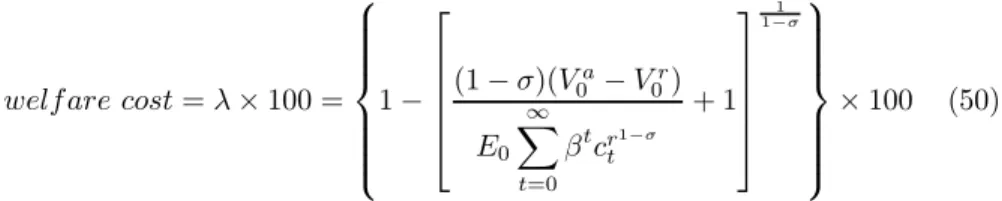
Welfare under the optimal policy is measured using equation (29). For the particular functional form for the period utility function given in equation (30), we have: V0a= · (1−λ)1−σ−1 1−σ ¸ E0 ∞ X t=0 βtcrt1−σ (49) Solving forλwe obtain the following expression for the welfare cost associ-ated with policy regimeavis-á-vis the reference policy regimer in percentage terms.
welf are cost=λ×100 =
1− (1−σ)(Va 0 −V0r) E0 ∞ X t=0 βtcr1−σ t + 1 1 1−σ ×100 (50)
We calculate welfare cost for a non-stochastic economy (at steady-state), usingfirst-order approximations and second-order approximations to the policy function. The following table shows the results for the non-stochastic and sto-chastic economy. For the latter, the initial conditions are given by the steady state values of the deterministic economy.
Table 3: Welfare under Fiscal Policy
Contemporaneous Taylor Rule
Steady State Welfare Welfare Cost
τk = 0.13 -466.1365
τk = 0 -455.7628 -3.62%
1st-order approximation -3.63%
2nd-order approximation -3.65%
Notice, that as expected, there are welfare gains by shifting to an optimal
fiscal policy. The welfare gains in the deterministic economy are 3.62 percent of consumption; for the stochastic economy using first-order approximations the gains are 3.63 percent; and for the economy with second-order approximations, they are 3.65 percent. Notice that the welfare gains we compute are almost the same, independent of using afirst or a second-order approximation. And they are also the same if we are considering a non-stochastic or a stochastic economy. So, an explanation for the deterministic economy is also valid for the stochastic economy.
The welfare gains in the non-stochastic economy are realized by reducing the capital tax to its optimal level, thus the capital in the economy increases. Agents optimally substitute labor with capital, as the labor tax remainsfixed. Of course the reduction in labor is not as high as the increase in capital. Labor reduces to 0.62073 and capital increases by 23 percent, as shown in table C1 in the appendix.
Notice that output increases by 7.18 percent. Consumption increases due to the income effect and leads to a higher demand of domestic money. Clearly, as the capital tax incomes for the government have decreased and government purchases arefixed, the government needs tofinance its purchases in some way, so it resorts to segniorage. In this way equilibrium is restored in the domestic money market.
There is also a push to foreign money, more consumption leads also to a higher demand for dollars. But notice, that dollars arefixed in the model, so a reduction in the devaluation rate is also needed to keep the demand of dollars
fixed. This is a typical mechanism in small open economies, the exchange rate always moves to restore the equilibrium.
The transmission mechanisms behind the welfare gains in the stochastic economy are the same as in the deterministic economy. Ifind that here, as in the deterministic economy, output increases by 7 percent on average. Consumption and investment increase, while labor decreases. These results are based on means and medians as shown in table C2 in the appendix.
The third and four column of the table show the cyclical properties of the baseline economy and the optimal economy, respectively. Notice that volatilities increase for output, investment and the level of dollarization (DOL), in the optimal case, while they decrease for consumption, labor and real balances in domestic money.18 This result means that agents smooth consumption when
capital taxes are reduced to zero.
In summary, from the four variables that are arguments in the utility func-tion, only dollars remainfixed, while consumption, leisure and real balances in domestic money increase with the optimal policy, leading to the welfare gain reported above.
1 8The dollarization level (DOL) is defined as the ratio of real balances in dollars over total money (pesos plus dollars).
5.4
Welfare under Optimal Monetary Policy
The optimal monetary policy result developed in section four, states that the government must satiate the economy with real balances, in order to reach a zero nominal interest rate. In this environment, where government spending isfixed, generating a deflation means that the government will make an extensive use of the money printing machine, and so people will enjoy infinite real balances in local money. Of course in a 2MIUF model, as in a MIUF model, this represents an infinite utility and so an infinite welfare. So we can not get a precise measure of welfare in this setting.
Therefore, I see only what happens if the yearly inflation rate is reduced, say, by three percentage points. This reduction corresponds to a 0.8 percentage points of reduction in the quarterly nominal interest rate. The welfare gains are shown in table 4. Notice that there is no difference in gains between the deterministic economy and the stochastic economy in any case, welfare gains are 1.71 percent.
Table 4: Welfare under Monetary Policy
Contemporaneous Taylor Rule
Steady State Welfare Welfare Cost
π= 0.05 -466.1365
π= 0.02 -466.1115 -0.0084%
1st-order approximation -0.0084%
2nd-order approximation -0.0084%
These gains are small, when compared to gains associated with optimalfiscal policy, and compared to other works. For example, Cooley and Hansen [9] in a stochastic monetary economy, estimate the gains from eliminating moderate inflation of 5 and 10 percent to zero inflation and find gains in lifetime utility of 0.4 and 0.6 percent. Cavalcanti and Villamil [3] in a model with currency substitution, but without capitalfind that the welfare gains from reducing
in-flation from high levels, such as 25%, to the optimal level are very small (0.03 percent).19
The intuition for this result is simple. By reducing the inflation rate, there are three effects. First, by the Fisher equation, the nominal interest rate is reduced in the same proportion as the reduction in inflation. Second, by the equation of dollars demand, a reduction in inflation leads to a higher demand of dollars. In order to stop this, the devaluation rate is reduced in the same proportion as inflation. This allows the economy to maintain the stock of dollars
fixed. Third, and the main effect for welfare, is that a reduction in inflation leads to higher real balances in domestic money. In fact they increase by 34 percent. But of course real balances in local money are low weighted in the utility function (θ= 0.26), so the impact on utility is lower and it is diminished by the parameterϕ.
1 9In a many times cited paper, Lucas [19]finds that the gains from removing business cycles in the economy, are around 0.05 percent of permanent consumption.
It can be seen in table C1, that the National Accounts ratios are not af-fected by a reduction in inflation. In fact real variables are not affected with optimal monetary policies in this type of model, revisiting the classical result of money neutrality. In the stochastic economy (see table C2), the effects are the same, only mean and median values of real balances in domestic money increase, causing the level of dollarization to decrease.
It is also shown that the real balances in local money and the level of dol-larization become more volatile with lower levels of inflation. The correlations with output are also reported for each variable and all correlations are positive, except for real balances in domestic money. The level of dollarization has the higher correlation coefficient (0.7) while labor has the lowest (0.14).
5.5
Welfare under Optimal Fiscal and Monetary Policy
Here, I analyze the welfare gains associated with both optimalfiscal and mon-etary policy jointly. In other words I show how better is society is in terms of permanent consumption, if the government reduces the capital income tax to zero and at the same time, reduces the yearly inflation target to 2 percent. The results in table 5 show that welfare gains under both optimal policies are the highest. In the deterministic economy, welfare gains are in the order of 3.62 percent, while in the stochastic economy, they are in the order of 3.66 percent.
Table 5: Welfare under Fiscal and Monetary Policy
Contemporaneous Taylor Rule
Steady State Welfare Welfare Cost
τk = 0.13andπ= 0.05 -466.1365
τk = 0andπ= 0.02 -455.7378 -3.62%
1st-order approximation -3.64%
2nd-order approximation -3.66%
The last column of table C1 in the appendix presents the steady state values for all the variables and confirms our conclusion that welfare gains are mainly driven by real balances in local currency. Notice that the impact on real variables is exactly the same as when we were only considering a reduction in the capital tax. The ratios of consumption and government spending over output reduce by 3.35 percent and 6.7 percent respectively, while investment over output increases by 15 percent.
The reduction in the inflation target to 2 percent reduces the nominal interest rate from 2.8 percent to 2 percent, exactly in the same magnitude as in the case with optimal monetary policy only. The only variables that differ with the previous cases are the real balances in local money and the devaluation rate. This means that the effect comes from the currency demand equations (equations 40 and 41 in the deterministic economy). Now the devaluation rate has to decrease even more, because it has to compensate not only for the lower inflation rate, but also for the higher level of consumption. The devaluation rate reduces by 10 percentage points more than in the optimal monetary policy
case and this allows the economy to keep steady-state real balances in dollars at a value of 2.19.
By comparing the percentage increase of real balances in the three cases analyzed here, we can see how big the impact of optimal policies is on this variable. In the optimalfiscal policy case it was a 7 percent increase, in the optimal monetary case it was a 34 percent increase and in this last case it is a 44 percent increase. Naturally, this increase is explained by the reduction in inflation and the expansion of consumption. These two effects generate a pressure in the demand of local currency, to which the government responds by increasing its supply. So, agents have more domestic currency in their pockets, and this produces felicity to them (more utility). Thus the final effect is an important increase in welfare.
The same mechanism of transmission applies to the stochastic economy. The last column of table C2 in the appendix, shows that output, consumption, investment and labor follow the same pattern as in the optimalfiscal policy case. There is a high increase of real balances, not only in terms of the mean and the median, also in terms of the standard deviation. Again, as dollars remain
fixed and real balances in local currency increase, broad money increases and the dollarization level decreases to 77 percent. The volatility of this level also increases from 0.0075 to 0.013.
5.6
Sensitivity Analysis
It is important to consider money in the utility function, when one is analyzing welfare gains associated with particular policies, if these gains come primarily by the increase of real balances. The preceding results showed that the weight that money could have in the utility function do matter in explaining this welfare gains, so in this section I perform a sensitivity analysis with the parameterθ, which represents the weight that real balances in domestic currency and dollars have in the utility function.
The followingfigure shows the welfare gains associated with all the possible values that we can assign toθ (range between 0 and 1) for the three exercises considered, i.e. optimalfiscal policy, optimal monetary policy and both policies considered jointly at the same time.
Figure 1: Welfare Gains from Optimal Policies for Different Values of θ
Thefirst thing to note is that the curves for the cases in which optimalfiscal policy is being considered are far away from the curve in which only monetary policy is being considered. Second, the curves are almost flat, which means that welfare is not very sensitivity to the parameterθ, in particular when only optimal monetary policy is being considered. In that case, by increasing the value of θ, the welfare gains can increase up to a maximum value of 0.035 percent. This value corresponds to the non-dollarized case and is very similar to the magnitudes founded by Cavalcanti and Villamil [3].
When optimalfiscal policy is being considered, the curves are a little steeper and welfare gains are considerable. Notice that the economy is able to enjoy high welfare gains from both optimal policies applied jointly, but the main impact comes from fiscal policy. If we assign all the weight to the domestic money (θ = 1) then the welfare gain is around 4.1 percent. Of course, since welfare gains come from real balances in domestic currency, if we assign higher values for it in the utility function, welfare gains will be higher. This is the reason why the curves have negative slopes. Asθ increases, welfare gains also increase.
In this way, we can also establish a relation between partially dollarization and welfare gains. As the country, in this case Bolivia, becomes more dollarized, welfare gains associated with optimal policies are lower. In the opposite case, welfare gains are higher. So, there is a negative relation between partially
dollarization and welfare gains. Moreover, welfare gains depend mainly onfiscal policy.
6
Conclusion
I have characterized optimalfiscal and monetary policy in a dynamic general equilibrium model with currency substitution and capital. This model offers two important features. First, both monetary and fiscal policy are analyzed jointly in a model where there is capital accumulation; and second it is a two-monies-in-the-utility function (2MIUF) model. This characteristics turn out to be important in obtaining the theoretical and empirical results.
The theoretical model implies that an optimal monetary policy must follow the Friedman Rule, that is to set the nominal interest rate close to zero. In order to reach this objective in the context of a policy guided by rules, it is necessary tofix a target for the inflation as low as possible. This will allow to satiate the economy with real balances, in fact a deflation is needed to reach this objective completely. Then, the optimality of thefiscal policy advices the capital income tax be set at zero. This is a steady-state result, but also a dynamic result that holds in the transition to the long-run.
The only difference between the traditional Ramsey problem in a one cur-rency model, and this model, is that here there is a first-order condition for dollars where the inflation and devaluation rates appear. This converts the Ramsey problem, into a not only real variables problem. Prices are also now involved in the system. I do not characterize numerically the Ramsey problem, instead I compute the welfare gains associated with the optimal policies that are an implication of the solution to the Ramsey problem.
Certainly, this paper revisits thefirst results on this literature using a very simple model, although now the mode is to analyze these issues in new-keynesian frameworks. Nevertheless, the contribution of this paper is important, if one thinks that traditional results have been proved for partially dollarized economies and also important empirical results are obtained, using the second-order ap-proximation technique developed by Schmitt-Grohé and Uribe[24] to obtain the policy rules.
The numerical results can be attributed to partially dollarized economies, because I have been very careful to calibrate the model for a real partially dol-larized economy, which is the Bolivian economy. Other papers have calibrated monetary models with currency substitution, but using standard parameter val-ues.20
I calibrate the model for Bolivia, using quarterly data for the period 1990-2005. There are few models calibrated for Bolivia, and the most are in the old tradition of computational general equilibrium (CGE) models (see Thiele and Wiebelt [27] for a recent model). The only RBC model corresponds to Quiroz,
et.al.[26] which is more than ten years old. So, this paper is also a contribution for this type of models for Bolivia.
The most important result of the empirical section is that welfare gains under optimalfiscal policy are higher than the gains under optimal monetary policy. The case in which I analyze optimal fiscal and monetary policy jointly shows clearly that the main impact come from thefiscal side. The presence of capital and money in the same model also reinforce this effect, because all real variables move towards higher levels of welfare. The economy can enjoy higher levels of welfare by reducing the capital tax to zero than by reducing the inflation target. The following results are obtained for welfare gains: 3.65 percent of current consumption (permanent) when capital tax is zero, 0.0084 percent when the inflation target is reduced to 2 percent; and 3.66 percent when both the capital tax is reduced to zero and the inflation target is reduced to 2 percent which is very similar to the case where onlyfiscal policy is considered. These gains cor-respond to a stochastic Bolivian economy and are the same for the deterministic economy.
An important conclusion is that there is a negative relation between the weight that dollars have in the utility function and the welfare gains. This is another way to say that there is a negative relation between dollarization and welfare gains. Doing a sensitivity analysis with the parameter that weights currencies in the utility function, Ifind that for higher values of the weight of real balances in local currency, higher welfare gains can be obtained with an optimal fiscal policy, but not very high with optimal monetary policy. When considering both policies at the same time, welfare gains can go from a value of 3.5 percent to a value of 4.1 percent.
This work leaves open some lines for future research. It would be interesting to characterize exactly the Ramsey policies, this means that taxes might be endogeneized, in order to see its cyclical movements. I am sure that the standard results would hold: capital taxes will be very close to zero and labor taxes would be smooth. This is also a neoclassical model. It would be interesting to modify the model introducing sticky prices and imperfect competition to see if the results related to welfare and money neutrality still appear. Finally and particularly interesting for the Bolivian economy, the model could be used to inspect all kind of policy implications. For example, it could be used to analyze the impact of an increase in the capital tax, assuming that there is one sector that is intensive in this input (the hydrocarbons sector).
References
[1] Canzoneri, M. and Behzad Diba (1993). Currency Substitution and Ex-change Rate Volatility in the European Community, Journal of Interna-tional Economics, Vol. 35, pp: 351-365.
[2] Castro, J. F., Eduardo Morón and Diego Winkelried (2004) Assesing Fi-nancial Vulnerability in Partially Dollarized Economies. Universidad del Pacífico (mimeo).
[3] Cavalcanti, T. V. and Anne P. Villamil (2003) The Optimal Inflation Tax and Structural Reform,Macroeconomic Dynamics, Vol.7(3), pp: 333-362. [4] Chari, V.V. and Patrick Kehoe (1999). Optimal Fiscal and Monetary
Pol-icy. Handbook of Macroeconomics, edited by John Taylor and Michael Woodford. Vol. 1C, chapter 26, pp: 1873-1745. Elsevier, North Holland. [5] Chamley, C. (1986). Optimal Taxation of Capital Income in General
Equi-librium with Infinite Lives",Econometrica, Vol.54(3), pp: 607-622. [6] Chari, Christiano and Kehoe (1991) “Optimal Fiscal and Monetary Policy
: Some Recent Results”Journal of Money Credit and Banking Vol. 23, pp: 519-539.
[7] Chari, V.V., Lawrence Christiano and Patrick Kehoe (1994). Optimal Fiscal Policy in a Business Cycle Model, Journal of Political Economy,
Vol.102(4), pp: 617-652.
[8] Chari, V.V., Lawrence Christiano and Patrick Kehoe (1996). Optimality of the Friedman Rule in Economies with Distorting Taxes,Journal of Mone-tary Economics, Vol.37, pp:203-223.
[9] Cooley, T. F. and Gary D. Hansen (1991) The Welfare Costs of Moderate Inflation, Journal of Money, Credit and Banking, Vol. 23, pp:483-503. [10] Correia, I. and Pedro Teles (1996). Is the Friedman Rule Optimal When
Money is an Intermediate Good?,Journal of Monetary Economics, Vol. 38, pp: 223-244.
[11] Correia I., Juan Pablo Nicolini and Pedro Teles (2004). Optimal Fiscal and Monetary Policy: Equivalence Results, Bank of Portugal (mimeo).
[12] Imrohoroglu, S. (1994). GMM Estimates of Currency Substitution be-tween Canada and the U.S. dollar,Journal of Money, Credit and Banking, Vol.26(4), pp:792-807.
[13] Jones, L.E., Rodolfo E. Manuelli and Peter E. Rossi (1993). Optimal Tax-ation in Models of Endogenous Growth, Journal of Political Economy, Vol.101, pp:485-517.
[14] Kim, J. and Sunghyun Henry Kim (2003). Spurious Welfare Reversals in International Business Cycle Models. Journal of International Economics,
Vol. 60, pp: 471-500.
[15] Koop, G., M. H. Pesaran, and S. M. Potter (1996). Impulse Response Analysis in Nonlinear Multivariate Models, Journal of Econometrics, Vol. 74(1), pp:119—147.
[16] Kydland, F.E. and Edward Prescott (1982) Time to Build and Aggregate Fluctuations",Econometrica Vol.50, pp: 1345-1370.
[17] Ljungqvist, L. and Thomas J. Sargent (2004) Recursive Macroeconomic Theory, Second Edition, MIT Press.
[18] Lucas, R.E. and Nancy Stokey (1983) Optimal Fiscal and Monetary Policy in an Economy without Capital,Journal of Monetary EconomicsVol.12(1), pp:55-93.
[19] Lucas, R. Jr. (1987) Models of Business Cycles, Cambridge, M.A.: Black-well.
[20] Mendoza, E. (2000) On the Benefits of Dollarization when Stabilization Policy is not Credible and Financial Markets are imperfect. NBER Working Paper No.7824.
[21] Morales, J.A. (2003) Dollarization of assets and liabilities: problem or solu-tion? The case of Bolivia. Presentación del presidente del Banco Central de Bolivia en el Programa de SeminariosLa Vía hacia la prosperidad regional y global: Retos y oportunidades, organizado por el FMI, BM en Dubai, Emiratos Arabes Unidos.
[22] Schmitt-Grohe, S. and Martín Uribe (2004). Optimal Fiscal and Monetary Policy under Sticky Prices,Journal of Economic Theory, Vol.114, pp: 198-230.
[23] Schmitt-Grohe, S. and Martín Uribe (2004) Optimal Fiscal and Monetary Policy under Imperfect Competition, Journal of Macroeconomics, Vol.26 (June 2004), pp:183-209.
[24] Schmitt-Grohé, S. and Martín Uribe (2004) Solving Dynamic General Equi-librium Models using a Second-order Approximation to the Policy Function.
Journal of Economic Dynamics & Control, Vol.28, pp: 755-775.
[25] Schmitt-Grohé, S. and Martín Uribe (2004) Optimal Simple and Imple-mentable Monetary and Fiscal Rules. Manuscript, Duke University. [26] Quiroz, J.A., Francisco A. Bernasconi, Romulo A. Chumacero y Cesar I.
Revoredo (1991). Modelos y Realidad. Enseñando macroeconomía de los noventa.Revista de Análisis Económico, Vol.6(2). Ilades.
[27] Thiele Rainer and Manfred Wiebelt (2003) Attacking Poverty in Bolivia-Past Evidence and Future Prospects: Lessons from a CGE Analysis. Doc-umento de Trabajo No.06/03, IISEC-Universidad Católica Boliviana. [28] Vegh, C. (1988). The Optimal Inflation Tax in the Presence of Currency
Substitution,Journal of Monetary Economics, Vol. 41, pp:351-370. [29] Walsh, Carl E. (1998) Monetary Theory and Policy, The MIT Press.
Appendix
Appendix A: Optimality of the Friedman Rule
Here I explain in detail the proof of the Friedman rule.
u(ct, mt, dt,1−nt) =U(H(ct, mt, dt),1−nt)
Vm(t) = 0implies: (1+Φ) um(t)+Φ[ucm(t)ct+umm(t)mt+udm(t)dt−unm(t)nt] = 0 Vc(t) =θtimplies: (1+Φ) uc(t)+Φ[ucc(t)ct+umc(t)mt+udc(t)dt−unc(t)nt] = θt uc(t) =UH(H(ct, mt, dt),1−nt)Hc um(t) =UH(H(ct, mt, dt),1−nt)Hm ud(t) =UH(H(ct, mt, dt),1−nt)Hd then uc(t)ct+um(t)mt+ud(t)dt=UH(H(ct, mt, dt),1−nt) [Hcct+Hmmt+Hddt] uc(t)ct+um(t)mt+ud(t)dt=UHH (by homogeneity)
Then the second derivatives are:
uc(t) +ucc(t)ct+ucm(t)mt+ucd(t)dt=UHHHcH+UHHc
we can canceluc(t) =UHHc
ucc(t)ct+ucm(t)mt+ucd(t)dt=UHHHcH
and similarly
ucm(t)ct+umm(t)mt+udm(t)dt=UHHHmH
then we have:
(1 +Φ)UHHm+Φ[UHHHmH−UHnHmn] = 0 (1 +Φ)UHHc+Φ[UHHHcH+UHnHcn] =θt
Appendix B: Benchmark economy: Bolivian economy
In this appendix I want to show some characteristics of the general equilibrium model calibrated for Bolivia. Recall that the benchmark characteristics are:
Table B1: Model simulations: Correlations k π e i d A g c l n m k 1 π 0.936 1 e 0.686 0.832 1 i 0.74 0.876 0.962 1 d 0.252 0.09 0.013 -0.099 1 A -0.027 -0.036 0.284 0.24 -0.026 1 g -0.003 -0.004 0.022 0.022 0.021 0.027 1 c 0.878 0.751 0.57 0.553 0.662 0.113 0.008 1 l 0.618 0.486 0.181 0.152 0.777 -0.482 -0.006 0.769 1 n -0.618 -0.487 -0.181 -0.153 -0.777 0.482 0.006 -0.769 -1 1 m -0.192 -0.433 -0.684 -0.745 0.666 -0.334 -0.019 0.12 0.504 -0.504 1
Table B2: Cross Correlations with output
Cross correlation of output with
x(-3) x(-2) x(-1) x x(+1) x(+2) x(+3) Output 0.99632 0.99749 0.99869 1 0.99869 0.99749 0.99632 Consumption 0.99613 0.99718 0.99826 0.99936 0.99834 0.99732 0.99628 Investment 0.86514 0.8675 0.87029 0.87281 0.87237 0.87239 0.87197 Level of Doll. 0.9963 0.9973 0.99834 0.99938 0.99835 0.99734 0.9963 Labor 0.99598 0.99701 0.99807 0.99919 0.99813 0.99711 0.99608 Domestic M. 0.99169 0.9928 0.99399 0.99528 0.99469 0.99403 0.99332 Inflation 0.95732 0.9578 0.95787 0.95852 0.95681 0.95504 0.95326 Devaluation 0.98951 0.99035 0.991 0.99156 0.98997 0.98846 0.98693 Interest Rate 0.99491 0.99581 0.99668 0.99739 0.996 0.99466 0.99331 Technology 0.99607 0.99723 0.99843 0.99973 0.99851 0.9974 0.9963 Government 0.99537 0.9963 0.99734 0.99839 0.99749 0.99654 0.99549
Appendix C: Welfare Comparisons
I analyze the welfare gains associated with optimalfiscal and monetary policy for a deterministic and stochastic Bolivian economy.
Table C1: Deterministic Economy Comparisons
Variable τk= 0.13/π= 0.05 τk= 0 π= 0.02 τk= 0/π= 0.02
Consumption 0.21502 0.22274 0.21502 0.22274 Leisure 0.3791 0.37927 0.3791 0.37927 Labor 0.6209 0.62073 0.6209 0.62073 Real balances in domestic currency 0.44194 0.47421 0.59437 0.63778 Real balances in dollars 2.1978 2.1978 2.1978 2.1978 Capital 2,4148 2.975 2.4148 2.975 Inflation rate 0.012272 0.012272 0.0049629 0.0049629 Devaluation rate 0.012429 0.011265 0.0051184 0.0039632 Nominal interest rate 0.028359 0.028359 0.020934 0.020934 Gov. purchases 0.032501 0.032501 0.032501 0.032501 Technology 0.30119 0.30119 0.30119 0.30119 GDP 0.29409 0.31522 0.29409 0.31522 Consumption/GDP 0.73113 0.70661 0.73113 0.70661 Gov. Purchases/GDP 0.11051 0.10311 0.11051 0.10311 Investment/GDP 0.15951 0.18335 0.15951 0.18335 Level of Dollarization 0.83258 0.82253 0.78713 0.77508
Table C2: Stochastic Economy Comparisons
τk= 0.13/π= 0.05 τk= 0 π= 0.02 τk= 0/π= 0.02
Mean 0.29527 0.31619 0.29527 0.31619 Output Median 0.29543 0.31644 0.29543 0.31644 Stand.Dev. 0.01186 0.012156 0.01186 0.012156
Corr. with output 1 1 1 1
Mean 0.21481 0.22247 0.21481 0.22247 Consumption Median 0.21493 0.22259 0.21493 0.22259 Stand.Dev. 0.006683 0.0061518 0.006683 0.0061518 Corr. with output 0.5202 0.4695 0.5202 0.4695 Mean 0.047611 0.058433 0.047611 0.058433 Investment Median 0.046646 0.057739 0.046646 0.057739 Stand.Dev. 0.027102 0.027775 0.027102 0.027775 Corr. with output 0.21893 0.25664 0.21893 0.25664 Mean 0.83316 0.82292 0.7876 0.77532 Dollarization Median 0.83303 0.82264 0.78727 0.77476 Stand.Dev. 0.007554 0.0076512 0.013698 0.013228 Corr. with output 0.62119 0.60185 0.70631 0.69681 Mean 0.62175 0.62149 0.62175 0.62149 Labor Median 0.62186 0.62143 0.62186 0.62143 Stand.Dev. 0.007916 0.0074274 0.007916 0.0074274 Corr. with output 0.14497 0.24738 0.14497 0.24738 Mean 0.44029 0.47299 0.59356 0.63758 Real balances in Median 0.43932 0.47246 0.59 0.63435 domestic money Stand.Dev. 0.03143 0.031206 0.056902 0.055997