Inventories and Optimal Monetary Policy

CFCM

C

ENTRE

F

OR

F

INANCE

A

ND

C

REDIT

M

ARKETS

Working Paper 09/06

Inventories and Optimal

Monetary Policy

Thomas A. Lubik &

Wing Leong Teo

Produced By:

Centre for Finance and Credit Markets

School of Economics

Sir Clive Granger Building

University Park

Nottingham

NG7 2RD

Tel: +44(0) 115 951 5619

Fax: +44(0) 115 951 4159

enquiries@cfcm.org.uk

Inventories and Optimal Monetary Policy

∗

Thomas A. Lubik

Federal Reserve Bank of Richmond

Wing Leong Teo

National Taiwan University

October 2009

Abstract

We introduce inventories into a standard New Keynesian Dynamic Stochastic Gen-eral Equilibrium (DSGE) model to study the effect on the design of optimal monetary policy. The possibility of inventory investment changes the transmission mechanism in the model by decoupling production fromfinal consumption. This allows for a higher degree of consumption smoothing since firms can add excess production to their in-ventory holdings. We consider both Ramsey optimal monetary policy and a monetary policy that maximizes consumer welfare over a set of simple interest rate feedback rules. Wefind that in contrast to a model without inventories, Ramsey-optimal monetary pol-icy in a model with inventories deviates from complete inflation stabilization. In the standard model, nominal price rigidity is a deadweight loss on the economy, which an optimizing policymaker attempts to remove. With inventories, a planner can reduce consumption volatility and raise welfare by accumulating inventories and letting prices change as an equilibrating mechanism. Wefind alsofind that the application of simple rules comes very close to replicating Ramsey optimal outcomes.

JEL Classification: E24; E32; J64.

Key Words: Ramsey policy, New Keynesian model

∗_{We are grateful to Andreas Hornstein, Pierre Sarte, Alex Wolman, and Nadezhda Maleyeva, whose}

comments greatly improved the paper. Part of this research were conducted while Lubik was the Geoffrey

Harcourt Visiting Professor at the University of Adelaide. He wishes to thank the members of the Economics Department for their hospitality. The views expressed in this paper are those of the authors and should not necessarily be interpreted as those of the Federal Reserve Bank of Richmond or the Federal Reserve System.

†_{Research Department, Federal Reserve Bank of Richmond. P.O. Box 27622, Richmond, VA 23261.}

Email: thomas.lubik@rich.frb.org.

‡_{Department of Economics, National Taiwan University, 21 Hsu Chow Road, Taipei 100, Taiwan. Phone:}

1

Introduction

It has long been recognized that inventory investment plays a large role in explainingfl uc-tuations in real GDP, although it makes up only a small fraction of the latter. Blinder and Maccini (1991) document that in a typical recession in the U.S., the fall in inventory investment accounts for 87% of the decline in output despite being only one half of 1 percent of real GDP. A lot of research has been trying to explain how this seemingly insignificant component of GDP has such a disproportionate role in business cycle fluctuations.1 How-ever, surprisingly few studies have focused on the conduct of monetary policy when firms can invest in inventories. In this paper we attempt to fill this gap by investigating how inventory investment affects the design of optimal monetary policy.

We employ the simple New Keynesian model which has become the benchmark for analyzing monetary policy from both a normative and a positive perspective. We introduce inventories into the model by assuming that the inventory stock facilitates sales, as suggested in Bils and Kahn (2000). Wefirst establish that the dynamics, and therefore the monetary transmission mechanism, differ between the models with and without inventories for a given behavior of the monetary authority. Monetary policy is then endogenized by assuming that policymakers solve an optimal monetary policy problem.

Wefirst compute the optimal Ramsey policy. A Ramsey planner maximizes the welfare of the agents in the economy taking into account the private sector’s optimality conditions. By doing so, the planner chooses a socially optimal allocation. While this does not neces-sarily bear any relationship to the typical conduct of monetary policymakers, it provides a useful benchmark. Subsequently, we study optimal policy when the planner is constrained to implement simple rules. That is, we specify a set of rules that let the policy instrument, the nominal interest rate, respond to target variables such as the inflation rate and output. The policymaker chooses the respective response coefficients that maximize welfare. Op-timal rules of this kind may be preferable to Ramsey plans from an actual policymaker’s perspective since they can be operationalized and are easier to communicate to the public. Our most interestingfinding is that Ramsey-optimal monetary policy deviates from full inflation stabilization in our model with inventories. This stands in contrast to the standard

1

New Keynesian model. In the latter framework, perfectly stable inflation is optimal since movements in prices represent deadweight costs to the economy. Introducing inventories modifies that basic calculus since holding inventories allowsfirms to smooth sales over time with concomitant effects on consumption. This change in the economy’s propagation mech-anism can require, however, movements in labor input. Moreover, output and consumption need no longer coincide as firms can invest in inventory holdings, which is similar to cap-ital in that it provides future consumption opportunities. Changes in prices serve as the equilibrating mechanism for the competing goals of reducing consumption volatility and of avoiding price adjustment costs. The inventory specification therefore contains something akin to an inflation-output trade-off. Consequently, the optimal policy no longer fully sta-bilizes inflation. The second importantfinding concerns the efficacy of implementing simple rules. Similar to most of the optimal policy literature, we show that simple rules can come exceedingly close to the socially optimal Ramsey policy in welfare terms.

Our paper relates to two literatures. First, the amount of research on optimal monetary policy in the New Keynesian framework is very large already, and we do not have much to contribute conceptually to the modeling of optimal policy. Schmitt-Grohé and Uribe (2007) is a recent important and comprehensive contribution. A main conclusion from this literature is that optimal monetary policy will choose to almost perfectly stabilize inflation. In environments with various nominal and real distortions, this policy prescription becomes slightly modified, but nevertheless perseveres. We thus contribute to the optimal policy literature by demonstrating that the results carry over to a framework with another, previously unconsidered modification to the basic framework in the form of inventories.

The study of inventory investment has a long pedigree, which we cannot do full jus-tice here. Much of the earlier literature, as surveyed in Blinder and Maccini (1991), was concerned with identifying the determinants of inventory investment, such as aggregate de-mand, and expectations thereof, or the opportunity costs of holding inventories. Most work in this area was largely empirical using semi-structural economic models, with West (1986) being a prime example.2 Almost in parallel to this more explicitly empirical literature, inventories were introduced into real business cycle models. The seminal paper by Kydland

2_{A more recent example of applying structural econometric techniques to partial equilibrium inventory}

and Prescott (1982) introduces inventories directly into the production function. More re-cent contributions include Christiano (1988), Fisher and Hornstein (2000), and Khan and Thomas (2007). The latter two papers especially build a theory of a firm’s inventory be-havior on the microfoundation of an S-s environment. The focus of these papers is on the business cycle properties of inventories, in particular the high volatility of inventory investment relative to GDP and the countercylicality of the inventory-sales ratio, both of which are difficult to match in typical inventory models. In an important paper, Bils and Khan (2000) demonstrate that time-varying and countercyclical mark-ups are crucial for capturing this comovement pattern.

This insight lends itself to considering inventory investment within a New Keynesian framework since it features interplay between marginal cost, inflation, and monetary policy, which might therefore be a source of inventoryfluctuations.3 _{Recently, several papers have}

introduced inventories into New Keynesian models. Jung and Yun (2005) and Boileau and Letendre (2008) both study the effects of monetary policy from a positive perspective. The former combines Calvo-type price setting in a monopolistically competitive environment with the approach to inventories as introduced by Bils and Kahn (2000). The use of the Calvo-approach to modeling nominal rigidity allows these authors to discuss the importance of strategic complementarities in price setting. Boileau and Letendre (2008), on the other hand, compare various approaches to introducing inventories in a sticky-price model. This paper is differentiated from these contributions by its focus on the implications of inventories as a transmission mechanism for optimal monetary policy.

The rest of the paper is organized as follows. In the next section we develop our New Keynesian model with inventories. Section 2 analyzes the differences between the standard New Keynesian model and our specification with inventories. We calibrate both models and compare their implications for business cycle fluctuations. We present the results of our policy exercises in Section 3, which also includes a robustness analysis with respect to changes in the parameterization. Section 4 concludes with a brief discussion of the main results and suggestions for future research.

3_{Incidentally, Maccini et al. (2004)find that an inventory model with regime switches in interest rates is}

quite succesful in explaining inventory behavior despite much previous empirical evidence to the contrary. The key to this result is the exogenous shift in interest rate regimes, which lines up with breaks in U.S. monetary policy.

2

The Model

We model inventories in the manner of Bils and Kahn (2000) as a mechanism for facilitating sales. Whenfirms face unexpected demand, they can simply draw down their stock of pre-viously produced goods and do not have to engage in potentially more costly production. This inventory specification is embedded in an otherwise standard New Keynesian environ-ment. There are three types of agents: monopolistically competitivefirms, a representative household, and the government. Firms face price adjustment costs and use labor for the production of finished goods which can be sold to households or added to the inventory. Households provide labor services to the firms and engage in intertemporal consumption smoothing. The government implements monetary policy.

2.1

Firms

The production side of the model consists of a continuum of monopolistically competitive

firms, indexed by i_∈[0,1]. The production function of afirm iis given by:

yt(i) =ztht(i), (1)

where yt(i) is output of firm i, ht(i) is labor hours used by firm i, and zt is aggregate productivity. We assume that it evolves according to the exogenous stochastic process:

lnzt=ρzlnzt−1+εzt, (2) whereεzt is an i.i.d. innovation.

We introduce inventories into the model by assuming that they facilitate sales as sug-gested by Bils and Kahn (2000).4 _{In their partial equilibrium framework, they posit a}

downward-sloping demand function for a firm’s product that shifts with the level of in-ventory available. As shown by Jung and Yun (2005), this idea can be captured in a New Keynesian setting with monopolistically competitive firms by introducing inventories directly into the Dixit-Stiglitz aggregator of differentiated products:

st= ÃZ 1 0 µ at(i) at ¶μ θ st(i)(θ−1)/θdi !θ/(θ−1) , (3)

4_{This approach is consistent with a stockout avoidance motive. Wen (2005) shows that it explains the}

wherestare aggregate sales, st(i) arefirm-specific sales, andatand at(i)are, respectively, the aggregate and firm-specific stocks of goods available for sales. θ > 1 is the elasticity of substitution between differentiated goods, and μ > 0 is the elasticity of demand with respect to the relative stock of goods. Holding inventories helps firms to generate greater sales at a given price since they can rely on the stock of previously produced goods when, say, demand increases. Note, however, that a firm’s inventory matters only to the extent that it exceeds the aggregate level. In a symmetric equilibrium, having inventories does not help a firm to make more sales, but it affects, as we shall see later, the firm’s optimality condition for inventory smoothing.

Cost minimization implies the following demand function for sales of goodi:

st(i) = µ at(i) at ¶μµ Pt(i) Pt ¶−θ st, (4)

wherePt(i) is the price of goodi, andPt is the price index for aggregate sales st:

Pt= µZ 1 0 µ at(i) at ¶μ Pt(i)1−θdi ¶1/(1−θ) . (5)

A firm’s sales are thus increasing in its relative inventory holdings and decreasing in its relative price. The inventory term can alternatively be interpreted as a taste shifter, which

firms invest in to capture additional demand (see Kryvtsov and Midrigan, 2009). Finally, the stock of goods available for salesat(i) evolves according to:

at(i) =yt(i) + (1−δ) (at−1(i)−st−1(i)), (6)

whereδ_∈(0,1)is the rate of depreciation of the inventory stock. It can also be interpreted as the cost of carrying the inventory over the period.

Each firm faces quadratic costs for adjusting its price relative to the steady state gross inflation rateπ: φ₂³ Pt(i)

πPt−1(i)−1

´2

st, withφ >0, andπ ≥1the steady state gross inflation rate. Note that the costs are measured in units of aggregate sales instead of output sincest is the relevant demand variable in the model with inventories. Firmi’s intertemporal profit function is then given by:

Et ∞ X τ=0 ρ_t,t+τ " Pt+τ(i)st+τ(i) Pt+τ − Wt+τht+τ(i) Pt+τ − φ 2 µ Pt+τ(i) πPt+τ−1(i)− 1 ¶2 st+τ # , (7)

where Wt is the nominal wage, andρt,t+τ is the aggregate discount factor that a firm uses to evaluate profit streams.

Firm i chooses its price Pt(i), labor input ht(i) and stock of goods available for sales

at(i) to maximize its expected intertemporal profit (7), subject to the production function (1), the demand function (4), and the law of motion forat(i) (6). Thefirst order conditions are: φ µ Pt(i) πPt−1(i)− 1 ¶ st πPt−1(i) = (1₋θ)st(i) Pt +Etρt,t+1 ∙ φ µ Pt+1(i) πPt(i) − 1 ¶ st+1Pt+1(i) πP2 t(i) + (1₋δ)θst(i) Pt(i) mct+1(i) ¸ , (8) Wt Pt =ztmct(i), (9) and mct(i) =μ Pt(i) Pt st(i) at(i) + (1₋δ) µ 1₋μst(i) at(i) ¶ Etρt,t+1mct+1(i), (10)

wheremct(i) is the Lagrange multiplier associated with the demand constraint (4). It can also be interpreted as real marginal cost.

Equation (8) is the optimal price setting condition in our model with inventories. It resembles the typical optimal price setting condition in a New Keynesian model with convex costs for price adjustment (e.g., Krause and Lubik, 2007), except that marginal cost now enters the optimal pricing condition in expectations because of the presence of inventories. In this model, the behavior of marginal cost mc can be interpreted from two different directions. As captured by Equation (9), it is the ratio of the real wage to the marginal product of labor, which in the standard model is equal to the cost of producing an additional unit of output. Alternatively, it is the cost of generating an additional unit of goods available for sale, which can either come out of current production or out of (previously) foregone sales. This in turn reduces the stock of goods available for sales in future periods, which would eventually have to be replenished through future production. This intertemporal trade-offbetween current and future marginal cost is captured by Equation (10).

2.2

Household

We assume that there is a representative household in the economy. It maximizes expected intertemporal utility, which is defined over aggregate consumption5 ct and labor hours ht:

E0 ∞ X t=0 βt " ζ_tlnct− h1+_t η 1 +η # , (11)

whereη _≥0is the inverse of the Frisch labor supply elasticity.

ζ_t is a preference shock and is assumed to follow the exogenous AR(1) process:

lnζ_t=ρ_ζlnζ_t−1+εζ,t, (12) where0< ρ_ζ<1and εζ,t is an i.i.d. innovation.

The household supplies labor hours to firms at the nominal wage rate Wt and earns dividend income Dt (which is paid out of firms’ profit) from owning the firms. It can purchase one-period discount bonds Bt at a price of 1/Rt, where Rt is the gross nominal interest rate. Its budget constraint is:

Ptct+Bt/Rt≤Bt−1+Wtht+Dt. (13)

The first-order conditions for the representative household’s utility maximization problem are: hη_t = ζt ct Wt Pt , (14) ζ_t ct =βRtEt µ ζ_t+1 ct+1 Pt Pt+1 ¶ , (15)

Equation (14) equates the real wage, valued in terms of the marginal utility of consumption, to the disutility of labor hours. Equation (15) is the consumption-based Euler equation for bond holdings.

2.3

Government and Market Clearing

In order to close the model, we also need to specify the behavior of the monetary authority. The main focus of the paper is on the optimal monetary policy in the New Keynesian

5_{Consumption can be thought of as a Dixit-Stiglitz aggregate as is typical in New Keynesian models. We}

model with inventories. In the next section, however, we briefly compare our specification to the standard model without inventories in order to assess whether introducing inventories significantly changes the model dynamics. We do this conditional for a simple, exogenous interest rate feedback rule that has been used extensively in the literature:

e

Rt=ρRet−1+ψ1πet+ψ2yet+εR,t, (16)

where a tilde over a variable denotes its log deviation from its deterministic steady state.ψ₁

andψ₂ are monetary policy coefficients, and0< ρ <1is the interest smoothing parameter.

εR,tis a zero mean innovation with constant variance. It is often interpreted as a monetary policy implementation error. Finally, we impose a symmetric equilibrium, so that thefi rm-specific indicesican be dropped. In addition, we assume that bonds are in zero net supply,

Bt = 0. Market clearing in the goods market requires that consumption together with the cost for price adjustment equals aggregate sales:

st=ct+ φ 2 ³_πt π −1 ´2 ct. (17)

3

Analyzing the E

ff

ects of Monetary Policy

The main focus of this paper is how the introduction of inventories into an otherwise stan-dard New Keynesian framework changes the optimal design of monetary policy. However, we begin by briefly comparing the behavior of the model with and without inventories to as-sess the changes in the dynamic behavior of output and inflation, given the exogenous policy rule (16). The standard New Keynesian model differs from our model with inventories in the following respects. First, there is no explicit intertemporal trade-offin terms of marginal cost as in Eq. (10). This implies, secondly, that the driving term in the Phillips-curve (8) is current marginal cost, as defined by Eq. (9). Finally, in the standard model, consumption, output, sales and goods available of sales arefirst-order equivalent. We note, however, that the standard specification is not nested in the model with inventories in the sense that the equation system for the latter reduces to the former for a specific parameterization.

3.1

Calibration

The time period corresponds to a quarter. We set the discount factorβ to0.99. Since price adjustment costs are incurred only for deviations from steady state inflation, its value is

irrelevant for first-order approximations of the model’s equation system, but plays a role when we perform the optimal policy analysis. We therefore setπ = 1.0086to be consistent with the average post-war quarter-over-quarter inflation rate. In the baseline calibration, we choose a fairly elastic labor supply and setη= 1, which is a common value in the literature and corresponds to quadratic disutility of hours worked. We impose a steady-state mark-up of 10% which implies θ = 11. The price adjustment cost parameter is then calibrated so that η(θ₋1)/φ = 0.1, as in Ireland (2004). This is a typical value for the coefficient on marginal cost in the standard New Keynesian Phillips curve.6 The parameters of the monetary policy rule are chosen to be broadly consistent with the empirical Taylor-rule literature for a unique equilibrium. That is, ψ₁ and ψ₂ are set to 0.45 and 0, respectively, while the smoothing parameterρ= 0.7. This choice corresponds to an inflation coefficient of0.45/0.3 = 1.5that obeys the Taylor-principle. We specify the policy rule in this manner since it allows us to analyze later on the effects of inertial and super-inertial rules with

ρ_≥1.

The persistence of the technology shock and the preference shock are both set to ρ_z =

ρ_ζ = 0.95. The standard deviation of the productivity innovation is then chosen such as to match the standard deviation of HP-filtered U.S. GDP of 1.61%. This yields a value of

σz = 0.005. We set the standard deviation of the preference shocks at 3 times the value of the former, which is consistent with empirical estimates from a variety of studies (e.g. Ireland, 2004). In the same manner, we choose a standard deviation of the monetary policy shock of0.003. The parameters related to inventories,μandδ, are calibrated following Jung and Yun (2005). Specifically, the elasticity of demand with respect to the stock of goods available for sales μ= 0.37, while the depreciation rate of the inventory stock δ = 0.01.

3.2

Do Inventories Make a Di

ff

erence?

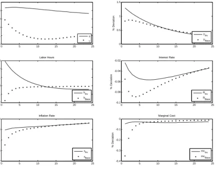
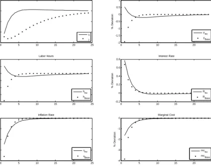
To get an idea how the introduction of inventories changes the model dynamics we compare the responses of some key variables to technology, preference, and monetary policy shocks for the specification with and without inventories. The impulse responses are found in Figures 1 to 3, respectively. In the Figures, the label ‘Base’ refers to the responses under the specification without inventories, while ‘Inv’ indicates the inventory specification. The

6_{This value is also consistent with an average price duration of about 4 quarters in the Calvo-model of}

key qualitative difference between the two models is the behavior of labor hours. In response to a persistent technology shock, labor increases in the model with inventories, while it falls in the standard New Keynesian model before quickly returning to the steady state.7 _{In the}

latter,firms can increase production even when economizing on labor because of the higher productivity level. There is further downward pressure on labor since the productivity shock raises the real wage. Higher output is reflected in a drop in prices which is drawn out over time due to the adjustment costs, and marginal cost falls strongly.

The presence of inventories, however, changes this basic calculus as firms can use in-ventories to take advantage of current low marginal cost.. With inventory accumulation

firms need not sell the additional output immediately, which prompts them to increase la-bor input. Consequently, output rises by more than in the standard model and the excess production is put in inventory. The stock of goods available for sales thus rises, whereas the sales-to-stock ratio γ_{t ≡} st/at falls. This is also reflected in the (albeit small) fall in marginal cost, which is, however, persistent and drawn out. In other words, firms use in-ventories to take advantage of current and future low marginal cost. Inflation moves in the same direction as in the standard model, but is much smoother, as the increased output does not have to be priced immediately. This behavior is just theflip side of the smoothing of marginal cost.

In response to a preference shock, hours move in the same direction in both models. However, the response with inventories is smaller since firms can satisfy the additional demand out of their inventory holdings, which therefore does not drive up marginal cost by as much. Compared to the standard model, firms do not have to resort to increases in price or labor input to satisfy the additional demand. Inventories are thus a way of smoothing revenue over time, which is also consistent with a smoother response of inflation. The dynamics following a contractionary policy shock are qualitatively similar to those of technology shocks in terms of comovement. Sales in the inventory model fall, but output and hours increase to take advantage of the falling marginal cost. All series are again noticeably smoother when compared to the standard model.

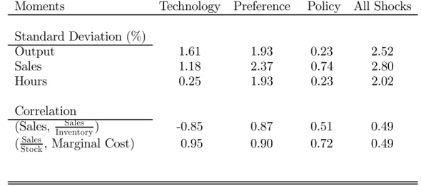
We now briefly discuss some business cycle implications of the inventory model.8 Table

7_{Chang et al. (2008) also emphasize that in the presence of nominal rigidities labor hours can increase}

in response to a persistent technology shock whenfirms hold inventories.

1 shows selected statistics for key variables. A notable stylized fact in U.S. data is that production is more volatile than sales. We find that our inventory model replicates this observation in the case of productivity shocks, that is, output is 30% more volatile. This implies that consumption, which is equal to sales in our linearized setting, is also less volatile than GDP. The introduction of inventories is thus akin to the modeling of capital and investment in breaking the tight link between output and consumption embedded in the standard New Keynesian model. However, the model has counterfactual implications for the comovement of inventory variables. Sales are highly negative correlated with the sales-inventory ratio, whereas in the data the two series comove slightly positively and are at best close to uncorrelated. This finding can be overturned when either preference or policy shocks are used, both of which imply a strong positive comovement. However, in the latter case, sales are counterfactually more volatile than output. When all shocks are considered together, wefind that comovement between the inventory variables and positive, but not unreasonably so, while sales are slightly more volatile than output.

The model also has implications for inflation dynamics. Most notably, inflation is less volatile in the inventory specification than in the standard model. In the New Keynesian model, inflation is driven by marginal cost, and hence the standard model predicts that the two variables are highly correlated. In the data, however, proxies for marginal cost, such as unit labor cost or the labor share comove only weakly with inflation. This has been a chal-lenge for empirical studies of the New Keynesian Phillips curve. Our model with inventories may, however, improve the performance of the Phillips curve in two aspects. First, marginal cost smoothing translates into a smoother, and thus more persistent inflation path; second, the form and the nature of the driving process in the Phillips-curve equation changes, as is evident from equations (8) and (10). The latter equation predicts a relationship between marginal cost and the sales-to-stock ratio γ which changes the channel by which marginal cost affects inflation dynamics.9

We can tentatively conclude that a New Keynesian model with inventories presents a modified set of trade-offs for an optimizing policymaker. In the standard model optimal policy is such that both consumption and the labor supply should be smoothed, and price

9_{This is further and more formally empirically investigated in Lubik and Teo (2009), who suggest that}

adjustment costs minimized. In the inventory model, these objectives are still relevant since they affect utility in the same manner, but the channel through which this can be achieved is different. Inventories allow for a smoother adjustment path of inflation, which should help contain the effects of price stickiness, while the consumption behavior depends on the nature of the shocks. We now turn to an analysis of optimal policy with inventories.

4

Optimal Monetary Policy

The goal of an optimizing policymaker is to maximize a welfare function subject to the con-straints imposed by the economic environment and subject to assumptions about whether the policymaker can commit or not to the chosen action. In this paper, we assume that the optimizing monetary authority maximizes the intertemporal utility function of the house-hold subject to the optimal behavior chosen by the private sector and the economy’s feasi-bility constraints. Furthermore, we assume that the policymaker can credibly commit to the chosen path of action and does not reoptimize along the way. We consider two cases. For our benchmark, we assume that the monetary authority implements the Ramsey optimal policy.10 We then contrast the Ramsey policy with an optimal policy that is optimized over a generic linear rule of the type used in the simulation analysis above.

We can alternatively interpret the policymaker’s actions as minimizing the distortions in the model economy. In a typical New Keynesian setup as ours, there are two distortions. The first is the suboptimal level of output generated by the presence of monopolistically competitivefirms. The second distortion arises from the presence of nominal price stickiness, as captured by the quadratic price adjustment cost function, which is a deadweight loss to the economy. In the standard model, the optimal policy is therefore to perfectly stabilize inflation at the steady state level. Introducing inventories does not change this basic calculus as the inventory mechanism does not introduce another distortion, but simply changes the transmission mechanism to shocks. We would therefore expect an optimal policy to deliver stabilized inflation as well. As we have seen above, however, inventories break the tight link in the standard model between consumption, output and thus labor hours. While in the standard model, there is no trade-offbetween smoothing consumption and labor, in the

1 0_{See Khan et al. (2003), Levin et al. (2006) and Schmitt-Grohé and Uribe (2007) for wide-ranging and}

model with inventories consumption equals sales and is decoupled from current production and hours. We will now investigate whether this additional wedge matters quantitatively for optimal policy.

4.1

Welfare Criterion

We use expected lifetime utility of the representative household at time zero, V₀a, as the welfare measure to evaluate a particular monetary policy regime a:

V₀a_≡E0 ∞ X t=0 βt " ζ_tlnC_ta₋(h a t) 1+η 1 +η # . (18)

As in Schmitt-Grohé and Uribe (2007), we compute the expected lifetime utility conditional on the initial state being the deterministic steady state for given sequences of optimal choices of the endogenous variables and exogenous shocks. Our welfare measure is in the spirit of Lucas (1987) and expresses welfare as a percentage Θ of steady state consumption that the household is willing to forgo to be as well offunder the steady state as under a given monetary policy regimea. Θcan then be computed implicitly from:

∞ X t=0 βt ∙ ζln ∙µ 1₋ Θ 100 ¶ c ¸ − h 1+η 1 +η ¸ =V₀a, (19)

where variables without time subscripts denote the steady state of the corresponding vari-ables.11 Note that a higher value ofΘcorresponds to lower welfare. That is, the household would be willing to give up Θ% of steady state consumption to implement a policy that delivers the same level of welfare as the economy in the absence of any shocks. This also captures the notion that business cycles are costly because they imply fluctuations that a consumption-smoothing and risk-averse agent would prefer not to have.

4.2

Optimal Policy

We compute the Ramsey policy by formulating a Lagrangian problem, in which the gov-ernment maximizes the welfare function (18) of the representative household subject to the private sectors’ first-order conditions and the market-clearing conditions of the economy. The optimality conditions of this Ramsey policy problem can then be obtained by diff er-entiating the Lagrangian with respect to each of the endogenous variables and setting the

1 1_{We assume that the policymaker chooses the same steady state inflation rate for all monetary policies}

derivatives to zero. This is done numerically by using the Matlab procedures developed by Levin and Lopez-Salido (2004). The welfare function is then approximated around the distorted, non-Pareto-optimal steady state. The source of steady state distortion is the inefficient level of output due to the presence of monopolistically competitivefirms.

In our second optimal policy case, we follow Schmitt-Grohé and Uribe (2007) and con-sider optimal, simple and implementable interest rate rules. Specifically, we consider rules of the following type:

e

Rt=ρRet−1+ψ1Eteπt+i+ψ2Etyet+i, i=−1,0,1. (20)

The subscriptiindicates that we consider forward-looking (i= 1), contemporaneous (i= 0), and backward-looking rules (i=₋1). Following the suggestion in Schmitt-Grohé and Uribe (2007), we focus on values of the policy parameters ρ, ψ₁, and ψ₂ that are in the interval

[0,3]. Note that this rule also allows for the possibility that the interest rate is super-inertial; that is, we assumeρcan be larger than 1. In order tofind the constrained-optimal interest rate rule, we search for combinations of the policy coefficients that maximize the welfare criterion. As in Schmitt-Grohé and Uribe (2007), we impose two additional restrictions on the interest rate rule: (i) the rule has to be consistent with a locally unique rational expectations equilibrium; (ii) the interest rate rule cannot violate2σR< R, whereσRis the unconditional standard deviation of the gross interest rate whileRis its steady state value. The second restriction is meant to approximate the zero bound constraint on the nominal interest rate.12

4.3

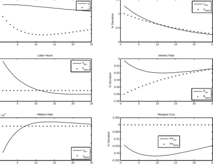
Ramsey Optimal Policy

A key feature of the standard New Keynesian set-up is that Ramsey-optimal policy com-pletely stabilizes inflation. Price movements represent a deadweight loss to the economy because of the existence of adjustment costs.13 An optimizing planner would, therefore, at-tempt to remove this distortion. This insight is borne out by the impulse response functions for the standard model without inventories in Figure 4. Inflation does not respond to the technology shock, nor do labor hours or marginal cost as per the New Keynesian Phillips

1 2_{If R is normally distributed 2σ}

R < R implies that there is a 95% chance that R will not hit the

zero-bound.

1 3_{In a framework with Calvo price setting the deadweight loss comes in form of relative price distortions}

curve. The path of output simply reflects the effect of increased and persistent productivity. The Ramsey planner takes advantage of the temporarily high productivity and allocates it straight to consumption without feedback to higher labor input or prices. The planner could have reduced labor supply to smooth the time path of consumption. However, this would have a level effect on utility due to lower consumption, positive price adjustment cost, via the feedback from lower wages to marginal cost, and increased volatility in hours. The solution to this trade-offis thus to bear the brunt of higher consumption volatility.

The possibility of inventory investment, however, changes this rationale (see Figure 4). In response to a technology shock, output increases by more compared to the model without inventories, while consumption, which is first-order equivalent to sales, rises less. Ramsey optimal policy can induce a smoother consumption profile by allowing firms to accumulate inventories. Similarly, the planner takes advantage of higher productivity in that he induces the household to supply more labor hours. Inflation is now no longer completely stabilized as the lower increase in consumption leads to an initial decline in inflation. Inventories thus serve as a savings vehicle that allows the planner to smooth out the impact of shocks. The planner incurs price adjustment costs and disutility from initially high labor input. The benefit is a smoother and more prolonged consumption path than would be possible without inventories. The model with inventories therefore restores something akin to an output-inflation trade-offin the New Keynesian framework.

The quantitative differences between the two specifications are small, however. Table 2 reports the welfare costs and standard deviations of selected variables for the two versions of the model under Ramsey optimal policy. The welfare costs of business cycles in the standard model are vanishingly small when only technology shocks are considered and undistinguish-able from the specification with inventories. The standard deviation of inflation is zero for the model without inventories while it is slightly higher for the model with inventories. This is consistent with the evidence from the impulse responses and highlights the differences between the two model specifications. Note also that consumption is less volatile in the model with inventories than in the standard model, which reflects the increased degree of consumption smoothing in the former.14

1 4_{This is consistent with the simulation results reported in Schmitt-Grohé and Uribe (2007) in a model}

with capital. They alsofind that full inflation stabilization is no longer optimal, since investment in capital

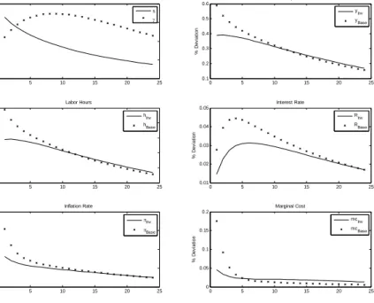
Figure 5 depicts the impulse responses to the preference shock under Ramsey optimal policy. Inflation and marginal cost are fully stabilized in the standard model, which the planner achieves through a higher nominal interest rate that reduces consumption demand in face of the preference shock. At the same time, the planner lets labor input go up to meet some of the additional demand. In contrast, Ramsey policy for the inventory model can allow consumption to increase by more sincefirms can draw on their stock of goods for sale. Consequently, output and labor increase by less for the inventory model. Similarly to the case of the technology shock, optimal policy does not induce complete inflation stabilization as it uses the inventory channel to smooth consumption. This is confirmed by the simulation results in Table 2, which show the Ramsey-planner trading offvolatility between inflation, consumption and labor when compared to the standard model.

Interestingly, eliminating business cycles and imposing the steady state allocation is costly for the planner in the presence of preference shocks that multiply consumption. This is evidenced by the negative entries for the welfare cost in both model specifications. In other words, agents would be willing to pay the planner0.05% of their steady state consumption

not to eliminate preference-driven fluctuations. This stems from the fact that, although

fluctuations per se are costly in welfare terms for risk-avers agents, they can also induce comovement between the shocks and other variables that have a level effect on utility. Specifically, preference shocks comove positively with consumption due to an increase in demand. This positive comovement is reflected in a positive covariance between these two variables. In our second-order approximation to the welfare functions this overturns the negative contribution to welfare from consumption volatility.

When we consider both shocks together, the differences between the two specifications are not large in welfare terms and with respect to the implications for second moments. Inflation and consumption are more volatile in the inventory version, while labor is less volatile compared to standard specification. We also compare Ramsey optimal policy with inventories to a policy of fully stabilizing inflation only (as opposed to using the utility-based welfare criterion from above). Panel C of Table 2 shows that the latter is very close to the Ramsey policy. The welfare difference between the two policies is small, less than 0.001 percentage points of steady state consumption. The effects of inventories can be seen in the slightly higher volatility of consumption and labor under the full inflation stabilization

policy. Inventory investment allows the planner to smooth consumption more compared to the standard model, and the mechanism is a change in prices. Although price stability feasible, the planner chooses to incur adjustment cost to reduce the volatility of consumption and labor.

4.4

Optimal Policy with a Simple and Implementable Rule

Ramsey optimal policy provides a convenient benchmark for welfare analysis in economic models. However, from the point of view of a policymaker, pursuing a Ramsey policy may be difficult to communicate to the public. It may also not be operational in the sense that the instruments used to implement the Ramsey policy may not be available to the policymaker. For instance, in a market economy the government cannot simply choose allocations as a Ramsey plan might imply. The literature has therefore focused on finding simple and implementable rules that come close to the welfare-outcomes implied by Ramsey policies (see Schmitt-Grohé and Uribe, 2007).

We therefore investigate the implications for optimal policy conditional on the simple rule (20). Panel A of Table 3 shows the constrained-optimal interest rate rules for the model without inventories with all shocks considered simultaneously. The rule that delivers highest welfare is a contemporaneous rule, with a smoothing parameterρ= 1and reaction coefficients on inflation ψ₁ and outputψ₂ of 3 and 0, respectively.15 _{This is broadly}

con-sistent with the results of Schmitt-Grohé and Uribe (2007), where the constrained-optimal interest rate rule also features interest smoothing and a muted response to output. With-out interest-rate smoothing the welfare cost of implementing this policy increases, which is exclusively due to a higher volatility of inflation.

On the other hand, the difference between the constrained-optimal contemporaneous rule and the Ramsey policy is small, less than 0.001 percentage points. This confirms the general consensus in the literature that simple rules can come extremely close to Ramsey optimal policies in welfare terms. The characteristics of constrained-optimal backward-looking and forward- backward-looking rules are similar to the contemporaneous rule, i.e., they also feature full interest smoothing and no output response. The welfare difference between the constrained-optimal contemporaneous rule and the other two rules are also small.

1 5

Turning to the model with inventories, we report the results for the constrained-optimal rules in Panel B of Table 3. All rules with interest smoothing deliver virtually identical results, but strictly dominate any rule without smoothing. As before, the coefficient on output is zero, while the policymakers implement a strong inflation response. The main difference to the Ramsey outcome is that inflation is slightly less volatile, while output is more volatile. This again confirms the findings in other papers that a policy rule with a fully inertial interest rate and a hawkish inflation response delivers almost Ramsey-optimal outcomes.

4.5

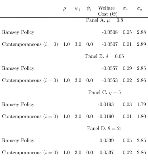
Sensitivity Analysis

We now investigate the robustness of our optimal monetary policy results to alternative parameter values. The results of alternative calibrations are reported in Table 5, where we only document results for the rule that comes closest to the Ramsey benchmark. In the robustness analysis, we change one parameter at a time while holding all other parameters at their benchmark values. The overall impression is that in all alternative calibrations the optimal simple rule comes close to the Ramsey policy, and that the relative welfare rankings for the individual rules established in the benchmark calibration is unaffected. Specifically, inertial rules tend to dominate rules with a lower degree of smoothing.

Wefirst look at the implications of alternative values for the two parameters related to inventories: the elasticity of demand with respect to the stock of goods available for salesμ

and the depreciation rate of the inventory stockδ. As in Jung and Yun (2005), we consider the alternative valueμ= 0.8. Since sales now respond more elastically to the stock of goods available for sale, the inventory channel becomes more valuable as a consumption-smoothing device and inflation becomes more volatile under a Ramsey policy. The best simple rule has contemporaneous timing and comes very close to the Ramsey policy in terms of welfare. The optimal rule is inertial and strongly reacts to inflation only. The volatility of inflation is lower than under the Ramsey policy and closer to that of the optimally simple rule with the benchmark calibration. This suggests that the response coefficients of the optimal rule are insensitive to changes in elasticity parameter μ, and that the Ramsey planner can exploit the changes in the transmission mechanism in a way that the simple rule misses. The quantitative differences are small, however.

In the next experiment, we increase the depreciation rate of the inventory stock to

δ= 0.05. It is at this value that Lubik and Teo (2009)find that the inclusion of inventories has a marked effect on inflation dynamics in the New Keynesian Phillips curve. Panel B of Table 5 shows that the preferred rule is again contemporaneous, but the differences between the alternatives are very small. Interestingly, Ramsey policy leads to a volatility of inflation that is almost an order of magnitude higher than in the benchmark case, which is consistent with thefindings in Lubik and Teo (2009).

The benchmark calibration imposed a very elastic labor supply with η= 1. The results of making the labor supply much more inelastic by setting η = 5 are depicted in Panel C of the table. For this value, the differences to the benchmark are most pronounced. In par-ticular, the volatility of output declines substantially across the board, which is explained by the difficulty with which firms change their labor input. The best simple rule is con-temporaneous, but the differences to the other rules are vanishingly small. Optimal policy puts again strong weight on inflation, with the optimal rule being inertial. Another diff er-ence to the benchmark parameterization is that the welfare cost of no interest smoothing is also much bigger for η = 5.16 Finally, we also report results for calibration with a lower steady state mark-up of 5%, which corresponds to a value of θ= 21. The qualitative and quantitative results are mostly similar to the benchmark results.

In summary, the results from the benchmark calibration are broadly robust. Under a Ramsey policy full inflation stabilization is not optimal, while the best optimal simple rule exhibits inertial behavior on interest smoothing and a strong inflation response. The welfare differences between alternative calibrations are very small, with the exception of changes in the labor supply elasticity. A less elastic labor supply reduces the importance of the inventory channel to smooth consumption by making it more difficult to adjust employment and output in the face of exogenous shocks.

5

Conclusion

We introduce inventories into an otherwise standard New Keynesian model that is com-monly used for monetary policy analysis. Inventories are motivated as a way to generate

1 6_{The welfare cost of no interest smoothing is 0.0088 for η = 5, while it is 0.0021 for the benchmark}

sales for firms. This changes the transmission mechanism of the model which has reper-cussions for the conduct of optimal monetary policy. We emphasize two main findings in the paper. First, we show that full inflation stabilization is no longer the Ramsey-optimal policy in the simple New Keynesian model with inventories. While the optimal planner still attempts to reduce inflation volatility to zero since it is a deadweight loss for the economy, the possibility of inventory investment opens up a trade-off. In our model, production needs no longer be consumed immediately, but can be put into inventory to satisfy future demand. An optimizing policymaker therefore has an additional channel for welfare-improving con-sumption smoothing, which comes at the cost of changing prices and deviations from full inflation stabilization. Our secondfinding confirms the general impression from the litera-ture that simple and implementable optimal rules come close to replicating Ramsey-policies in welfare terms.

This paper contributes to a growing literature on inventories within the broader New Keynesian framework. However, evidence on the usefulness of including inventories to improve the model’s business cycle transmission mechanism is mixed, as we have shown above. Future research may therefore delve deeper into the empirical performance of the New Keynesian inventory model, in particular on how modeling inventories affects inflation dynamics. Jung and Yun (2005) and Lubik and Teo (2009) proceed along these lines. A second issue concerns the way inventories are introduced into the model. An alternative to our setup is to add inventories to the production structure so that instead of smoothing sales, firms can smooth output. Finally, it would be interesting to estimate both model specifications with structural methods and compare their overallfit more formally.

References

[1] Bils, Mark, and James A. Kahn (2000): “What Inventory Behavior Tells Us About Business Cycles”.American Economic Review, 90(3), 458-481.

[2] Blinder, Alan S., and Louis J. Maccini (1991): “Taking Stock: A Critical Assessment of Recent Research on Inventories”.Journal of Economic Perspectives, 5(1), 73-96.

[3] Boileau, Martin, and Marc-André Letendre (2008): “Inventories, Sticky Prices, and the Persistence of Output and Inflation”. Manuscript.

[4] Chang, Yongsung, Andreas Hornstein, and Pierre-Daniel Sarte (2008): “On the Em-ployment Effects of Productivity Shocks: The Role of Inventories, Demand Elasticity and Sticky Prices”.Journal of Monetary Economics, forthcoming.

[5] Christiano, Lawrence J. (1998): “Why Does Inventory Investment Fluctuate So Much?”Journal of Monetary Economics, 21(2/3), 247-280.

[6] Fisher, Jonas D., and Andreas Hornstein (2000): “(S,s) Inventory Policies in general Equilibrium”.Review of Economic Studies, 67, 117-145.

[7] Ireland, Peter N. (2004): “Technology Shocks in the New Keynesian Model”. Review

of Economics and Statistics, 86(4), 923-936.

[8] Jung, YongSeung, and Tack Yun (2005): “Monetary Policy Shocks, Inventory Dynam-ics and Price-setting Behavior”. Manuscript.

[9] Khan, Aubhik, (2003): “The Role of Inventories in the Business Cycle”.Federal Reserve

Bank of Philadelphia Business Review, Third Quarter, 38-46.

[10] Khan, Aubhik, Robert G. King, and Alexander Wolman (2003): “Optimal Monetary Policy”.Review of Economic Studies, 70, 825-860.

[11] Khan, Aubhik, and Julia Thomas (2007): “Inventories and the Business Cycle: An Equilibrium Analysis of (S,s) policies”.American Economic Review, 97, 1165-1188.

[12] Krause, Michael U., and Thomas A. Lubik (2007): “The (Ir)relevance of Real Wage Rigidity in the New Keynesian Model with Search Frictions”. Journal of Monetary

Economics, 54(3), 706-727.

[13] Kryvtsov, Oleksiy, and Virgiliu Midrigan (2009): “Inventories and Real Rigidities in New Keynesian Business Cycle Models”. Manuscript.

[14] Kydland, Finn E., and Edward C. Prescott (1982): “Time to Build and Aggregate Fluctuations”.Econometrica, 50(6), 1345-1370.

[15] Levin, Andrew T., and David Lopez-Salido (2004): “Optimal Monetary Policy with Endogenous Capital Accumulation”. Manuscript.

[16] Levin, Andrew T., Aleksii Onatski, John C. Williams, and Noah Williams (2006): “Monetary Policy under Uncertainty in Micro-founded Macroeconometric Models”. In: Gertler, Mark, and Kenneth Rogoff (Eds.).NBER Macroeconomics Annual 2005. MIT Press, Cambridge, London, 229-287.

[17] Lucas, Robert (1987).Models of Business Cycles. Yrjö Johansson Lectures Series. Lon-don: Blackwell.

[18] Lubik, Thomas A., and Wing Leong Teo (2009): “Inventories, Inflation Dynamics and the New Keynesian Phillips Curve”. Manuscript.

[19] Maccini, Louis J., Bartholomew Moore, and Huntley Schaller (2004): “The Interest Rate, Learning, and Inventory Investment”.American Economic Review, 94(5), 303-1328.

[20] Maccini, Louis J., and Adrian Pagan (2008): “Inventories, Fluctuations and Business Cycles”. Manuscript.

[21] Ramey, Valerie A., and Kenneth D. West (1999): “Inventories”. In: John B. Taylor, Michael Woodford (eds.),Handbook of Macroeconomics, Volume 1, 863-923.

[22] Schmitt-Grohé, Stephanie, and Martín Uribe (2004): “Solving Dynamic General Equi-librium Models Using a Second-order Approximation to the Policy Function”.Journal

of Economic Dynamics and Control, 28, 755-775.

[23] Schmitt-Grohé, Stephanie, and Martín Uribe (2007): “Optimal, Simple and Imple-mentable Monetary and Fiscal Rules”.Journal of Monetary Economics, 54, 1702—1725.

[24] Wen, Yi (2005): “Understanding the Inventory Cycle”. Journal of Monetary

Eco-nomics, 52, 1533—1555.

[25] West, Kenneth D. (1986): “A Variance Bounds Test of the Linear Quadratic Inventory Model”.Journal of Political Economy, 94(2), 939-971.

Table 1: Business Cycle Statistics

Moments

Technology

Preference

Policy

All Shocks

Standard Deviation (%)

Output

1.61

1.93

0.23

2.52

Sales

1.18

2.37

0.74

2.80

Hours

0.25

1.93

0.23

2.02

Correlation

(Sales,

)

-0.85

0.87

0.51

0.49

(

, Marginal Cost)

0.95

0.90

0.72

0.49

Figure 1: Impulse Response Functions to Productivity Shock 0 5 10 15 20 25 -1.5 -1 -0.5 0 0.5 1 % D e vi a ti o n

Sales and Sales-Stock Ratio

s γ 0 5 10 15 20 25 0 0.5 1 1.5 % D e vi a ti o n Output yInv y Base 0 5 10 15 20 25 -0.2 -0.1 0 0.1 0.2 0.3 % D e vi a ti o n Labor Hours hInv hBase 0 5 10 15 20 25 -0.1 -0.08 -0.06 -0.04 -0.02 % D e vi a ti o n Interest Rate RInv RBase 0 5 10 15 20 25 -0.2 -0.15 -0.1 -0.05 0 % D e vi a ti o n Inflation Rate πInv πBase 0 5 10 15 20 25 -0.4 -0.3 -0.2 -0.1 0 % D e vi a ti o n Marginal Cost mc Inv mcBase

Table 2:

Welfare Costs and Standard Deviations under Ramsey Optimal Policy

Technology

Preference

All Shocks

Panel A: Model without Inventories

Welfare Cost (

Θ

)

0.0000

-0.0521

-0.0521

Standard Deviation (%)

Output

1.60

2.40

2.89

Inflation

0.00

0.00

0.00

Consumption

1.60

2.40

2.89

Labor

0.00

2.40

2.40

Panel B: Model with Inventories

Welfare Cost (

Θ

)

0.0000

-0.0529

-0.0529

Standard Deviation (%)

Output

1.73

2.28

2.86

Inflation

0.02

0.04

0.04

Consumption

1.45

2.60

2.97

Labor

0.24

2.28

2.29

Panel C: Full Inflation Stabilization

Welfare Cost (

Θ

)

0.0000

-0.0528

-0.0528

Standard Deviation (%)

Output

1.73

2.29

2.87

Inflation

0.00

0.00

0.00

Consumption

1.45

2.61

2.99

Labor

0.24

2.29

2.30

Table 3: Optimal Policy with a Simple Rule

ρ

ψ

ψ

Welfare

σ

σ

cost (

Θ

)

Panel A: Model without Inventories

Ramsey Policy

-0.0521

0.00

2.89

Optimized Rules

Contemporaneous (

i

= 0

)

Smoothing

1.00

3.00

0.00

-0.0520

0.04

2.89

No Smoothing

0.00

3.00

0.00

-0.0499

0.28

2.89

Backward (

i

=

₋

1

)

Smoothing

1.00

3.00

0.00

-0.0520

0.05

2.89

No Smoothing

0.00

3.00

0.00

-0.0501

0.27

2.90

Forward (

i

= 1

)

Smoothing

1.00

3.00

0.00

-0.0518

0.08

2.90

No Smoothing

0.00

3.00

0.00

-0.0496

0.30

2.90

Panel B: Model with Inventories

Ramsey Policy

-0.0529

0.04

2.86

Optimized Rules

Contemporaneous (

i

= 0

)

Smoothing

1.00

3.00

0.00

-0.0528

0.01

2.87

No smoothing

0.00

3.00

0.00

-0.0518

0.20

2.87

Backward (

i

=

₋

1

)

Smoothing

1.00

3.00

0.00

-0.0528

0.02

2.87

No smoothing

0.00

3.00

0.00

-0.0518

0.19

2.87

Forward (

i

= 1

)

Smoothing

1.00

3.00

0.00

-0.0528

0.02

2.87

No smoothing

0.00

3.00

0.00

-0.0517

0.20

2.87

Table 3: Optimal Policy for the Inventory Model

Alternative Calibration

ρ

ψ

ψ

Welfare

σ

σ

Cost (

Θ

)

Panel A.

μ

= 0

.

8

Ramsey Policy

-0.0508

0.05

2.88

Contemporaneous (

i

= 0

)

1.0

3.0

0.0

-0.0507

0.01

2.89

Panel B.

δ

= 0

.

05

Ramsey Policy

-0.0557

0.09

2.85

Contemporaneous (

i

= 0

)

1.0

3.0

0.0

-0.0553

0.02

2.86

Panel C.

η

= 5

Ramsey Policy

-0.0193

0.03

1.79

Contemporaneous (

i

= 0

)

1.0

3.0

0.0

-0.0190

0.01

1.80

Panel D.

θ

= 21

Ramsey Policy

-0.0539

0.05

2.85

Contemporaneous (

i

= 0

)

1.0

3.0

0.0

-0.0537

0.02

2.86

Figure 2: Impulse Response Functions to Preference Shock 0 5 10 15 20 25 0 0.2 0.4 0.6 0.8 % D e vi a ti o n

Sales and Sales-Stock Ratio

s γ 0 5 10 15 20 25 0.1 0.2 0.3 0.4 0.5 0.6 % D e vi a ti o n Output y Inv yBase 0 5 10 15 20 25 0.1 0.2 0.3 0.4 0.5 0.6 % D e vi a ti o n Labor Hours h Inv hBase 0 5 10 15 20 25 0.01 0.02 0.03 0.04 0.05 % D e vi a ti o n Interest Rate R Inv RBase 0 5 10 15 20 25 0 0.02 0.04 0.06 0.08 % D e vi a ti o n Inflation Rate πInv πBase 0 5 10 15 20 25 0 0.05 0.1 0.15 0.2 % D e vi a ti o n Marginal Cost mc Inv mcBase

Figure 3: Impulse Response Functions to Monetary Policy Shock 0 5 10 15 20 25 -3 -2 -1 0 1 % D e vi a ti o n

Sales and Sales-Stock Ratio

s γ 0 5 10 15 20 25 -2 -1.5 -1 -0.5 0 0.5 1 % D e vi a ti o n Output yInv y Base 0 5 10 15 20 25 -2 -1.5 -1 -0.5 0 0.5 1 % D e vi a ti o n Labor Hours hInv hBase 0 5 10 15 20 25 -0.2 0 0.2 0.4 0.6 0.8 % D e vi a ti o n Interest Rate RInv RBase 0 5 10 15 20 25 -0.8 -0.6 -0.4 -0.2 0 % D e vi a ti o n Inflation Rate πInv πBase 0 5 10 15 20 25 -4 -3 -2 -1 0 % D e vi a ti o n Marginal Cost mc Inv mcBase

Figure 4: Impulse Response Functions to Productivity Shock: Ramsey Policy 0 5 10 15 20 25 -1.5 -1 -0.5 0 0.5 1

Sales and Sales-Stock Ratio

% D e vi a ti o n s γ 0 5 10 15 20 25 0 0.5 1 1.5 Output % D e vi a ti o n yinv ybase 0 5 10 15 20 25 -0.1 0 0.1 0.2 0.3 Labor Hours % D e vi a ti o n h inv hbase 0 5 10 15 20 25 -0.06 -0.05 -0.04 -0.03 -0.02 -0.01 0 Interest Rate % D e vi a ti o n Rinv Rbase 0 5 10 15 20 25 -8 -6 -4 -2 0 2x 10 -3 Inflation Rate % D e vi a ti o n πinv πbase 0 5 10 15 20 25 -0.025 -0.02 -0.015 -0.01 -0.005 0 0.005 Marignal Cost % D e vi a ti o n mcinv mcbase

Figure 5: Impulse Response Functions to Preference Shock: Ramsey Policy 0 5 10 15 20 25 0 0.2 0.4 0.6 0.8

Sales and Sales-Stock Ratio

% D e vi a ti o n s γ 0 5 10 15 20 25 0.1 0.2 0.3 0.4 0.5 Output % D e vi a ti o n y inv ybase 0 5 10 15 20 25 0.1 0.2 0.3 0.4 0.5 Labor Hours % D e vi a ti o n h inv hbase 0 5 10 15 20 25 0 0.01 0.02 0.03 0.04 0.05 Interest Rate % D e vi a ti o n R inv Rbase 0 5 10 15 20 25 -6 -4 -2 0 2x 10 -3 Inflation Rate % D e vi a ti o n πinv πbase 0 5 10 15 20 25 -0.04 -0.03 -0.02 -0.01 0 0.01 0.02 Marignal Cost % D e vi a ti o n mc inv mcbase

Working Paper List 2008

Number Author Title

08/10 Marta Aloi, Manuel

Leite-Monteiro and Teresa Lloyd-Braga

Unionized Labor Markets and Globalized Capital Markets

08/09 Simona Mateut, Spiros Bougheas and Paul Mizen

Corporate trade credit and inventories: New evidence of a tradeoff from accounts payable and receivable

08/08 Christos Koulovatianos, Leonard J. Mirman and Marc Santugini

Optimal Growth and Uncertainty: Learning

08/07 Christos Koulovatianos, Carsten Schröder and Ulrich Schmidt

Nonmarket Household Time and the Cost of Children

08/06 Christiane Baumeister, Eveline Durinck and Gert Peersman

Liquidity, Inflation and Asset Prices in a Time-Varying Framework for the Euro Area

08/05 Sophia Mueller-Spahn The Pass Through From Market Interest Rates to Retail Bank Rates in Germany

08/04 Maria Garcia-Vega and Alessandra Guariglia

Volatility, Financial Constraints and Trade

08/03 Richard Disney and John Gathergood

Housing Wealth, Liquidity Constraints and Self-Employment

08/02 Paul Mizen and Serafeim Tsoukas What Effect has Bond Market Development in Asia had on the Issue of Corporate Bonds

08/01 Paul Mizen and Serafeim Tsoukas Modelling the Persistence of Credit Ratings When Firms Face Financial Constraints, Recessions and Credit Crunches

Working Paper List 2007

Number Author Title

07/11 Rob Carpenter and Alessandra Guariglia

Investment Behaviour, Observable Expectations, and Internal Funds: a comments on Cummins et al, AER (2006)

07/10 John Tsoukalas The Cyclical Dynamics of Investment: The Role of Financing and Irreversibility Constraints

07/09 Spiros Bougheas, Paul Mizen and Cihan Yalcin

An Open Economy Model of the Credit Channel Applied to Four Asian Economies

07/08 Paul Mizen & Kevin Lee Household Credit and Probability Forecasts of Financial Distress in the United Kingdom

07/07 Tae-Hwan Kim, Paul Mizen & Alan Thanaset

Predicting Directional Changes in Interest Rates: Gains from Using Information from Monetary Indicators

07/06 Tae-Hwan Kim, and Paul Mizen Estimating Monetary Reaction Functions at Near Zero Interest Rates: An Example Using Japanese Data

07/05 Paul Mizen, Tae-Hwan Kim and Alan Thanaset

Evaluating the Taylor Principle Over the Distribution of the Interest Rate: Evidence from the US, UK & Japan

07/04 Tae-Hwan Kim, Paul Mizen and Alan Thanaset

Forecasting Changes in UK Interest rates

07/03 Alessandra Guariglia Internal Financial Constraints, External Financial Constraints, and Investment Choice: Evidence From a Panel of UK Firms

07/02 Richard Disney Household Saving Rates and the Design of Public Pension Programmes: Cross-Country Evidence

Working Paper List 2006

Number Author Title

06/04 Paul Mizen & Serafeim Tsoukas Evidence on the External Finance Premium from the US and Emerging Asian Corporate Bond Markets

06/03 Woojin Chung, Richard Disney, Carl Emmerson & Matthew Wakefield

Public Policy and Retirement Saving Incentives in the U.K.

06/02 Sarah Bridges & Richard Disney Debt and Depression

06/01 Sarah Bridges, Richard Disney & John Gathergood

Housing Wealth and Household Indebtedness: Is There a 'Household Financial Accelerator'?

Working Paper List 2005

Number Author Title

05/02 Simona Mateut and Alessandra Guariglia

Credit channel, trade credit channel, and inventory investment: evidence from a panel of UK firms

05/01 Simona Mateut, Spiros Bougheas and Paul Mizen