Wasserstein Discriminant Analysis
R´
emi Flamary, Marco Cuturi, Nicolas Courty, Alain Rakotomamonjy
To cite this version:
R´
emi Flamary, Marco Cuturi, Nicolas Courty, Alain Rakotomamonjy. Wasserstein
Discrimi-nant Analysis. 2016.
<
hal-01377528
>
HAL Id: hal-01377528
https://hal.archives-ouvertes.fr/hal-01377528
Submitted on 7 Oct 2016
HAL
is a multi-disciplinary open access
archive for the deposit and dissemination of
sci-entific research documents, whether they are
pub-lished or not.
The documents may come from
teaching and research institutions in France or
abroad, or from public or private research centers.
L’archive ouverte pluridisciplinaire
HAL, est
destin´
ee au d´
epˆ
ot et `
a la diffusion de documents
scientifiques de niveau recherche, publi´
es ou non,
´
emanant des ´
etablissements d’enseignement et de
recherche fran¸
cais ou ´
etrangers, des laboratoires
publics ou priv´
es.
Wasserstein Discriminant Analysis
R´emi Flamary
Universit´e Cˆote d’Azur
Marco Cuturi
Kyoto University
Nicolas Courty
University of Bretagne Sud
Alain Rakotomamonjy
Rouen University
Abstract
Wasserstein Discriminant Analysis (WDA) is a new supervised method that can improve classification of high-dimensional data by computing a suitable linear map onto a lower dimensional subspace. Following the blueprint of classical Lin-ear Discriminant Analysis (LDA), WDA selects the projection matrix that maxi-mizes the ratio of two quantities: the dispersion of projected points coming from different classes, divided by the dispersion of projected points coming from the same class. To quantify dispersion, WDA uses regularized Wasserstein distances, rather than cross-variance measures which have been usually considered, notably in LDA. Thanks to the the underlying principles of optimal transport, WDA is able to capture both global (at distribution scale) and local (at samples scale) interac-tions between classes. Regularized Wasserstein distances can be computed using the Sinkhorn matrix scaling algorithm; We show that the optimization of WDA can be tackled using automatic differentiation of Sinkhorn iterations. Numerical experiments show promising results both in terms of prediction and visualization on toy examples and real life datasets such as MNIST and on deep features ob-tained from a subset of the Caltech dataset.
1
Introduction
Dimensionality reduction techniques can convert high-dimensional data with potentially redundant features into low-dimensional vectors [1, 2]. In doing so, dimensionality reduction can alleviate ensuing computations, and, ideally, extract relevant features out of noisy ones. Dimensionality reduction techniques come in all flavors: Some techniques only consider linear transformations of the data, whereas some extract features using nonlinear functions; Some of these techniques, such as PCA, are designed for unsupervised settings, whereas some can consider labeled data and fall in the supervised category. We consider in this paper linearandsupervised techniques. Within that category, two families of methods stand out: Given a dataset of pairs of vectors and labels
{(xi, yi)}i, the goal ofFisher Discriminant Analysis(FDA) and variants is to learn a linear mapP:
Rd →Rp,pd, such that the embeddings of these pointsPxican be easily discriminated using
linear classifiers. Mahalanobis metric learning(MML) methods proceed in the same way, except that the quality of the embeddingPis judged by the ability of thek-nearest neighbor algorithm to obtain good classification accuracy. Although both FDA and MML learn a mapP, their algorithms are shaped by the classifiers they use in their final phase.
FDA[3,§4.3] attempts to maximize w.r.t.Pthe sum ofalldistances||Pxi−Pxj0||between pairs of samples from different classesc, c0while minimizing the sum ofalldistances||Pxi−Pxj||between
pairs of samples within the same classc. Because of this, it is well documented that the performance of FDA degrades when class distributions are multimodal. Several variants have been proposed to
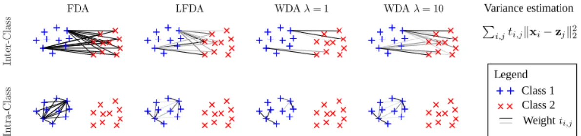
In t e r -C la s s FDA In t r a -C la s s
LFDA WDAλ= 1 WDAλ= 10
Legend Class 1 Class 2 Weight Variance estimation
Figure 1: Weights used for inter/intra class variances for FDA, Local FDA and WDA for different regularizationsλ. Only weights for two samples from class 1 are shown. The color of the link darkens as the weight grows. FDA computes a global variance with uniform weight on all pairwise distances, whereas LFDA focuses only on samples that lie close to each other. WDA relies on an optimal transport matrixT that matches all points in one class to all other points in another class. WDA has both a global (due to matching constraints) and local (due to transportation cost minimization) outlook on the problem, with a tradeoff controlled by the regularization strengthλ.
tackle this problem [3,§12.4]. For instance, a localized version of FDA was proposed in [4], which boils down to discarding in the computation all pairs of points that are not neighbors.
On the other hand, despite the fact that Mahalanobis metric learning (MML) was originally de-signed to operate with ak-nearest neighbor classifier, the first techniques that were proposed in that field [5] used aglobalcriterion, based on all pairs of points. Later on, variations that focused instead exclusively onclose-rangeinteractions, such as LMNN [6], were shown to be far more efficient.
Supervised dimensionality approaches stemming either from FDA or MML consider thuseither
globalorlocal interactions between points, but not both at the same time. We introduce in this work a novel approach that incorporatesbothglobal and local constraints. WDA can achieve this blend through the mathematics of optimal transport, which enforce that global and local aspects are taken into account when computing the weighttijthat regulates the influence of the distance||Pxi−Pxj||.
Indeed, such weights are decided by(i)making sure thatallpoints in one set are matched toall
points in the other set (global constraint);(ii)making sure that points are only matched on average to nearby points, thanks to the optimality of the transportation matrix (local cost). Our method has the added flexibility that it can interpolate between an exclusively global viewpoint (identical, in that case, to FDA), to a more local viewpoint with a global matching constraint (different, in that sense, to that of purely local tools such as LMNN or Local-FDA). In mathematical terms, we adopt the ratio formulation of FDA to maximize the ratio of the regularized Wasserstein distances between inter class populations and between the intra-class population with itself, when these points are consideredin their projected space:
max P∈∆ P c,c0>cWλ(PXc,PXc 0 ) P cWλ(PXc,PXc) (1) where∆ ={P= [p1, . . . ,pp] | pi ∈Rd,kpik2= 1 andp>i pj = 0fori6=j}is the Stiefel
manifold [7], the set of orthogonald×pmatrices;PXcis the matrix of projected samples from
classcandWλis the regularized Wasserstein distance proposed in [8]. We recover FDA when the entropic regularization strength is very large (smallλ). When, on the contrary, that regularization is weak, our approach tries to split two class distributions by, using loose language, making sure that their optimal matching distance is as large as possible. In that process, each point in one class is paired with another point in another class, and only that distance is maximized. Figure 1 illustrates how inter and intra-class distances are computed, and the difference in how data points interact locally when comparing Wasserstein discriminant analysis (WDA), a global approach such as FDA, and a purely local one such as Local-FDA [4].
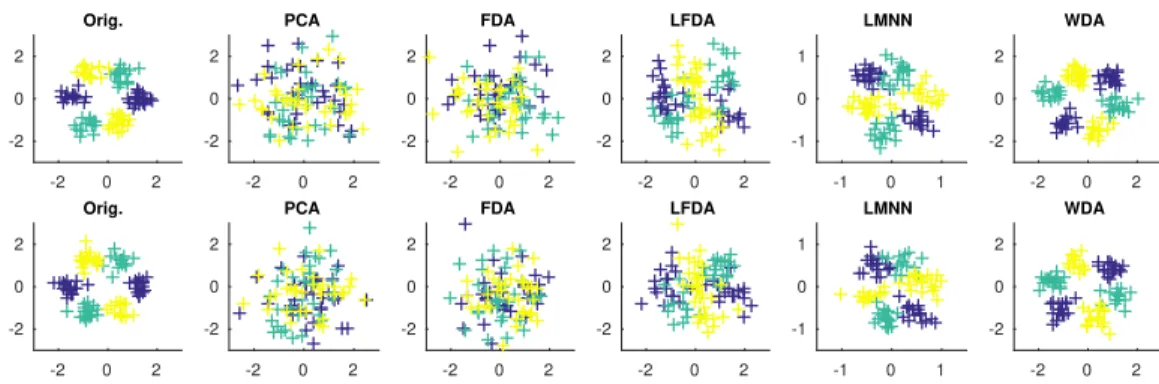
Another strong feature brought by regularized Wasserstein distances is that relations between sam-ples (as given by the optimal transport matrixT) are estimated in the projected space. This is an important difference compared to all previous local approaches which estimate local relations in the original space and make the hypothesis that these relations are unchanged after projection. Esti-mating local relations in the projected space leads to more robust results in the presence of noisy dimensions, as illustrated in Figure 2, on a simulated example containing 8 out of 10 features with
-2 0 2 -2 0 2 Train data Orig. -2 0 2 -2 0 2 PCA -2 0 2 -2 0 2 FDA -2 0 2 -2 0 2 LFDA -1 0 1 -1 0 1 LMNN -2 0 2 -2 0 2 WDA -2 0 2 -2 0 2 Test data Orig. -2 0 2 -2 0 2 PCA -2 0 2 -2 0 2 FDA -2 0 2 -2 0 2 LFDA -1 0 1 -1 0 1 LMNN -2 0 2 -2 0 2 WDA
Figure 2: Illustration of subspace learning methods on a nonlinearly separable 3-class toy example of dimensiond= 10with 2 discriminant features (shown on the left) and 8 Gaussian noise features. The projection ontop= 2for training (up) and test data (down) are reported for several subspace estimation methods.
only Gaussian noise. In this case, the 2D space estimated by our method is more discriminant than the local methods that rely on a noisy neighborhood estimation.
In what follows, we provide first background on regularized Wasserstein distances, present our Wasserstein-based discriminant analysis framework in§3 and discuss the optimization problem we tackle, which we solve using automatic differentiation. Numerical experiments that show the rele-vance of our approach are provided in§4.
2
Background on Wasserstein distances
Wasserstein distances, also known as earth mover distances, define a geometry over the space of probability measures using principles from optimal transport theory [9]. Recent computational ad-vances [8, 10] have made it scale to dimensions relevant to machine learning applications.
Notations and Definitions Letµ = 1nP
iδxi,ν = m1 Piδzi be two empirical measures with locations in Rd stored in the matrices X = [x1,· · · ,xn] andZ = [z1,· · · ,zm]. The squared
Euclidean distance between samples fromµandνis defined asMX,Z := [||xi−zj||22]ij ∈Rn×m. LetUnmbe the polytope ofn×mnonnegative matrices such that their row and column marginals are equal to1n/nand1m/mrespectively. Writing1nfor then-dimensional vector of ones,
Unm:={T∈Rn+×m : T1m=1n/n,TT1n=1m/m}.
Regularized Wassersein distance LethA, Bi:= tr(ATB)be the Frobenius dot-product of ma-trices. For λ ≥ 0, the regularized Wasserstein distance we adopt in this paper betweenµandν
is:
Wλ(µ, ν) :=Wλ(X,Z) :=hTλ,MX,Zi, (2) whereTλis the solution of an entropy-smoothed optimal transport problem,
Tλ:= argminT∈Unm λhT,MXZi −Ω(T), (3)
whereΩ(T)is the entropy ofTseen as a discrete joint probability distribution, namelyΩ(T) :=
−P
ijtijlog(tij). Note that problem (3) can be solved very efficiently using the Sinkhorn fixed
point iterations [8]. The solution of the optimization problem can be expressed as:
T= diag(u)e−λMdiag(v) =u1mT ◦e−λM◦1nvT, (4)
where◦stands for elementwise multiplication of matrices and the exponential is also applied ele-mentwise. The Sinkhorn iterations consist in updating left/right scaling vectorsuk andvk of the matrixK=e−λM. These updates take the following form for iterationk:
vk = 1m/m
KTuk−1, uk =
1n/n
Kvk (5)
with an initialization which will be fixed tou0=1
n. Because it only involves matrix products, the
Optimal transport for machine learning The geometry of the space of probability measures endowed with the Wasserstein metric has been recently considered in applied settings, notably to compute barycenters [11, 10], or generalizations of PCA [12]. Wasserstein distances have also been considered to carry out semi-supervised learning [13], domain adaptation [14], or to define new loss functions for multiclass classifiers [15]. A recent application related to ours is that of identifying univariate projections of high-dimensional probability distributions [16]. Contrary to our approach, this reference builds upon the closed form formulation of 1D-Wasserstein distances and was not designed to find subspaces of dimensionp >1.
3
Wasserstein Discriminant Analysis
In this section we discuss the optimization problem (1) and its relation to FDA. Then we propose an efficient approach for computing the gradient of the objective function.
Optimization problem In the remaining, to simplify notations, we define a separate empirical measure for each of the C classes: The samples of each class c are stored in matrices Xc; the
number of samples from classcisnc.
Using the definition (2) of the regularized Wasserstein distance, we can write the Wasserstein Dis-criminant Analysis optimization problem as
max P∈∆ ( J(P,T(P)) = P c,c0>chPTP,Cc,c 0 i P chPTP,Cc,ci ) (6) s.t.Cc,c0 =X i,j Ti,jc,c0(xci−xcj0)(xci−xcj0)T, ∀c, c0 andTc,c0 = argminT∈U ncnc0 λhT,MPXc,PXc 0i −Ω(T), which can be reformulated as
max
P∈∆ J(P,T(P)) (7)
s.t.T(P) = argminT∈Uncnc0 E(T,P) (8)
whereT={Tc,c0}c,c0 contains all the transport matrices between classes. The objective function
Jand the inner problem functionEdefined as
J(P,T(P)) = hP TP,C bi hPTP,C wi , E(T) = X c,c>=c0 λhTc,c0,M PXc,PXc0i −Ω(Tc,c 0 ) (9) whereCb =Pc,c0>cCc,c0 andCw =P
cCc,c are the between and within cross-covariance
ma-trices that depend onT(P). Optimization problem (7)-(8) is a classic bilevel optimization problem and it has a particular form that allows its resolution using gradient descent [17]. Indeed sinceT(P) is smooth and optimization problem (8) is strictly convex one can compute the gradient directlyw.r.t.
Pusing the chain rule as follows
∇PJ(P,T(P)) = ∂J(P,T) ∂P + X c,c0≥c ∂J(P,T) ∂Tc,c0 ∂Tc,c0 ∂P (10)
The first term in gradient (10) suppose thatTis constant and can be computed (Eq. 94-95 [18]) as
∂J(P,T) ∂P =P 2 σ2 w Cb− 2σ2 b σ4 w Cw (11) withσ2
w =hPTP,Cwiandσb2 = hPTP,Cbi. In order to compute the second term in (10), we
will separate the cases whenc=c0andc6=c0 since it corresponds to their position in the fraction. Their partial derivative is obtained directly from the scalar product and is a weighted vectorization of the transport cost matrix
∂J(P,T) ∂Tc,c06=c =vec 1 σ2 b MPXc,PXc0 , ∂J(P,T) ∂Tc,c =−vec σw2 σ4 b MPXc,PXc (12)
We will see in the remaining that the main difficulty stands in computing the Jacobian ∂Tc,c 0
∂P since
the optimal transport matrix is not available as a closed form. In the sequel, we solve this problem by means of an automatic differentiation approach wrapped around the Sinkhorn fixed point iteration algorithm.
Once the gradient is computed, we can use classical manifold optimization tools such as projected gradient [19] or a trust region algorithm as implemented in Manopt [20]. The latter toolbox in-cludes tools to optimize over the Stiefel manifold, notably automatic conversions from Euclidean to Riemannian gradients.
Relation to Fisher Discriminant Analysis We consider the limit behavior of WDA as λ ap-proaches0. In this case, we can see from Eq. (3) that the matrixTdoes not depends on the data. The solution T for each Wasserstein distance is the matrix that maximizes entropy, namely the uniform probability distributionT=nm1 1n,m. The cross-covariance matrices become thus
Cc,c0 = 1
ncnc0
X
i,j
(xci−xcj0)(xci−xcj0)T
and the matricesCwandCbcorrespond then to intra- and inter-class covariances as used in FDA.
Since these matrices do not depend on P, the optimization problem (1) boils down to the usual Rayleigh quotient which can be solved using a generalized eigendecomposition ofC−1
w Cb. When λ >0, the smoothed optimal transport promotes instead cross-covariance matrices that tend to favor local relations as illustrated in Figure 1.
Also note that the regularization parameter (λ < ∞) is required in the current formulation (1). Indeed, the classical Wasserstein distance of a discrete distribution with itself is0. The entropic regularization ensures that the mass of each sample is split among neighbors hence promoting a local variance estimation and avoiding a division by0in (1). If one wants to use the non-regularized Wasserstein distance, then the intra-class distance should be computed between two non-overlapping splits of the examples of each class which would also leads to non-zero distance.
Automatic Differentiation A possible way to compute the Jacobian∂Tc,c0/∂Pis to use the im-plicit function theorem as proposed in [21] for hyperparameter estimation. Although we have tried it, as detailed in supplementary material, this computational approach fails to scale because it re-quires inverting a very large matrix, and also assumes that the exact optimal transport Tcan be obtained, despite the fact that one only gets it after a finite number of Sinkhorn iterations. Following the gist of [22] (which do not differentiate Sinkhorn iterations but a more complex fixed point iter-ation designed to compute Wasserstein barycenters), we propose in this section to differentiate the transportation matrices obtained after running exactlyLSinkhorn iterations, with a predefinedL. WritingTk(P), for the solution obtained afterkiterations as a function ofPfor a givenc, c0pair,
Tk(P) = diag(uk)e−λMdiag(vk)
whereMis the distance matrix induced byP.TL(P)can then be directly differentiated: ∂Tk ∂P = ∂[uk1T m] ∂P ◦e −λM◦1 nvk T +uk1Tm◦ ∂e−λM ∂P ◦1nv k T +uk1T m◦e −λM◦∂[1nvk T] ∂P (13) Note that the recursion occurs asuk depends onvk whose is also related touk−1. The Jacobians that we need can then be obtained from Equation (5). For instance, the gradient of one component ofuk1T mat thej-th line is ∂uk j ∂P =− 1/n [Kvk]2 j X i ∂Kj,i ∂P v k i + X i Kj,i ∂vk i ∂P ,
while forvk, we have
∂vk j ∂P =− 1/m [KTuk−1]2 j X i ∂Ki,j ∂P u k−1 j + X i Ki,j ∂ukj−1 ∂P ,
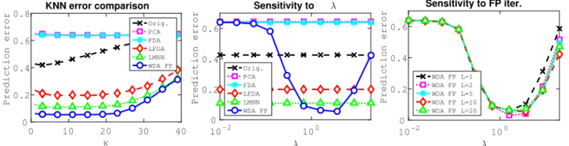
0 10 20 30 40 K 0 0.2 0.4 0.6 0.8 Prediction error KNN error comparison Orig. PCA FDA LFDA LMNN WDA FP 10-2 100 λ 0 0.2 0.4 0.6 Prediction error Sensitivity to λ Orig. PCA FDA LFDA LMNN WDA FP 10-2 100 λ 0 0.2 0.4 0.6 Prediction error Sensitivity to FP iter. WDA FP L=1 WDA FP L=2 WDA FP L=5 WDA FP L=10 WDA FP L=20
Figure 3: Prediction error on the simulated dataset with projection dimensionp= 2. (left) Error for a varyingKin the KNN classifier (middle) Evolution of WDA performance for different regular-ization parameter valuesλ(right) comparison of WDA performances as a function of the number of fixed point iterations.
and finally ∂Ki,j ∂P =−2Ki,jP(xi−x 0 j)(xi−x0j) T.
The Jacobian ∂∂TPk can be thus obtained by keeping track of all the Jacobians at each iteration and then by successive applying those equations. This approach is far cheaper than the implicit function theorem approach. Indeed, in this case, the computation of ∂∂TP is dominated by the complexity of computing ∂∂KP whose costs for one iteration isO(pn2d2)forn=m. The complexity is then linear inLand quadratic inn.
4
Numerical experiments
In this section we illustrate WDA on three datasets. First, we evaluate our approach on a simple simulated dataset with a 2-dimensional discriminant subspace that is known a priori. Then we apply WDA on MNIST and Caltech datasets. Note that in the spirit of reproducible research all the Matlab code will be made available to the community on Github and mloss.org upon publication.
Practical implementation In order to make the method less sensitive to the dimension and scal-ing of the data, we propose to use a pre-computed adaptive regularization parameterλc,c0 for each Wasserstein distances in (1). In practice we initializePwith the PCA projection, and we use it to find the followingλc,c0 =λ( 1
ncnc0 P i,jkPx c i −Px c0 jk
2)−1 between classcandc0. These val-ues are computeda priori and fixed in the remaining iterations, buth they will promote a similar regularization between inter and intra-class distances.
Simulated dataset This dataset has been designed to evaluate the ability of a subspace method to estimate a linear subspace when the classes are non-linearly separable. It is a 3-class problem in dimension d = 10where only the first two dimensions are discriminant and the remaining 8 contain Gaussian noise with the same variance as the discriminant dimensions. In the2discriminant features each class contains two modes that have centers positioned so that all the classes have the same mean at[0,0]. An example of samples in the discriminant dimensions is shown in the left part of Figure 2.
First, we depict in Figure 2, the samples projected in several subspaces with different approaches. We can see that for this dataset WDA seems to estimate the subspace with the best generalization property. To verify this trend, we compute the prediction errors of all the linear subspace methods with a K-Nearest-Neighbors classifier (KNN) forn = 100training examples andnt = 5000test examples in Figure 3. In this simulation, all prediction errors are averaged over 20 data generations and the neighbors parameters of LMNN and LFDA have been selected empirically to maximize performances (K = 5for LMNN andK = 1for LFDA). We can see in the left part of the figure that WDA and to a lesser extent LMNN can estimate a relevant subspace that is robust to the choice ofK. LFDA clearly outperforms PCA, Orig. and LDA since it can handle non-linearity but fails to attain the performances of LMNN and WDA. In the center plot, we illustrate the sensitivity of
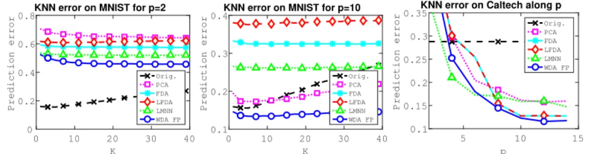
0 10 20 30 40 K 0 0.2 0.4 0.6 0.8 Prediction error
KNN error on MNIST for p=2
Orig. PCA FDA LFDA LMNN WDA FP 0 10 20 30 40 K 0.1 0.2 0.3 0.4 Prediction error
KNN error on MNIST for p=10
Orig. PCA FDA LFDA LMNN WDA FP 5 10 15 p 0.1 0.15 0.2 0.25 0.3 0.35 Prediction error
KNN error on Caltech along p Orig. PCA FDA LFDA LMNN WDA FP
Figure 4: (left) Averaged prediction error on MNIST with projection dimensionp= 2and (middle)
p= 10. (right) Averaged prediction error on the Caltech-256 dataset as a function ofp.
-100 0 100 -50 0 50 Train data PCA -50 0 50 -50 0 50 FDA -50 0 50 -50 0 50 LFDA -50 0 50 -50 0 50 LMNN -50 0 50 -50 0 50 WDA FP -40 -20 0 20 40 -40 -20 0 20 40 Test data -40 -20 0 20 40 -40 -20 0 20 40 -40 -20 0 20 40 -40 -20 0 20 40 -40 -20 0 20 40 -40 -20 0 20 40 -40 -20 0 20 40 -40 -20 0 20 40
Figure 5: 2D tSNE of the MNIST samples projected on p = 10 for different approaches. (up)
training set (down) test set.
WDAw.r.t.the regularization parameterλ. WDA returns the best performance on almost a full order of magnitude which suggests that a coarse validation can be performed in practice. The right part of Figure 3 shows the performance of the WDA with fixed point gradient (WDA FP) for different values of the number of inner iterationsL. We can see that even if this parameter leads to different performances on large values ofλit still leads to the best overall performances even for smallL. The variability between the curves comes from the non-convexity of the objective function, since each descent direction might lead to a different stationary point.
MNIST dataset. Our aim on this dataset is to measure how robust our approach is when only few training samples are available in high-dimension. To this end, we drawn= 1000samples for train-ing and report the KNN prediction error as a function ofkfor the different subspace methods when projecting ontop= 2andp= 10dimensions (resp. left and middle plots of Figure 4). In order to leverage the impact of a random choice of the initial distribution, the reported scores are averages of 20 realizations of the same experiment. We also limit the analysis toL = 10as the number of fixed point iterations. As expected, whenp = 2there is an important loss of information which leads to large classification errors compared to a KNN in the original space (Orig.). Nevertheless, WDA seems to be the method that finds the best 2D subspace. Whenp= 10, WDA finds a better subspace than the original space which suggests that all the discriminant information available in the training dataset has been extracted efficiently. Conversely, LFDA and LMNN struggle in finding a relevant subspace in this configuration. We believe that this is due to the small number of training samples and the fact that those approaches look at local relationship whereas the Wasserstein dis-tance is a global measure that can be regularized to better avoid overfitting and to better capture local informations. In addition to better prediction performance, we want to emphasize that in this con-figuration WDA leads to a dramatic compression of the data from 784 to 10 features while keeping the discriminative information.
To gain a better understanding of the corresponding embedding, we project the data from the 10-dimensional space to a 2-10-dimensional one using tSNE, that is a classic nonlinear projection method used for visualizing high dimensional samples for instance in deep architectures [23]. In order to
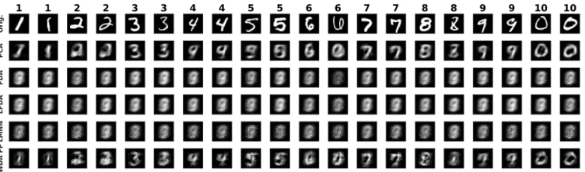
Figure 6: Image reconstruction after projection in the subspaces for test samples. The title on top of each column corresponds to the class of the sample.
be able to compare the embeddings, we first apply tSNE on samples in the PCA space and use it as an initialization for all the other methods. The resulting 2D projections for both training and testing samples are shown in Figure 5. Here we can clearly see the overfitting of FDA, LFDA and LMNN that separate accurately the training samples but fail to separate the test samples.
We finally compare in Figure 6 the different reconstructions induced by the adjoint projection oper-ator. One can see that contrary to the other discriminative methods, our method preserves a coherent spatial information related to the class, which illustrates again the generalization capability of WDA. The means that the estimated subspace is both generative as for PCA and discriminative thanks to the use of a proper divergence between discrete distributions.
Caltech dataset In this experiment, we use a subset described in [24] from the Caltech-256 image collection [25]. The dataset uses features that are the output of the DeCAF deep learning architec-ture [24]. More precisely, they are extracted as the sparse activation of the neurons from the 6th fully connected layer of a convolutional network trained on imageNet and then fine-tuned for the considered visual recognition task. As such, they form vectors of 4096 dimensions. In this setting, 500 images are considered for training, and the remaining portion of the dataset for testing (623 images). There are 9 different classes in this dataset. We examine in this experiment how the pro-posed dimensionality reduction performs when changing the subspace dimensionality (right plot in Figure 4). For this problem, the regularization parameterλof WDA was empirically set to10−2and we use early stopping at10iterations for WDA. The K from KNN was to set to3which is a com-mon standard setting for this classifier. The reported results are averaged over 10 realizations of the same experiment. Whenp≥5, WDA already finds a subspace which gathers all the discriminative information from the original space. In this experiment LMNN reaches a better subspace for small
pvalues but WDA is the best performing method forp≥6. Those results highlight the potential interest for using WDA as linear dimensionality reduction layers in neural-nets architecture.
5
Conclusion
This work presents the Wasserstein Discriminant Analysis, a new and original linear discriminant subspace estimation method. Based on the framework of Wasserstein distances, which measure a global similarity between empirical distributions, WDA operates by separating distributions of different classes in the subspace, while maintaining a coherent structure at a class level. To this extent, the use of regularization in the Wasserstein formulation allows to effectively bridge a gap between a global coherency and the local structure of the class manifold. This comes at a cost of a difficult optimization of a bilevel program, for which we showed that a naive computation of the gradient is achievable but computationally too costly in real settings. We proposed instead an efficient method that relies on differentiating the map obtained after a finite number of iterations of the Sinkhorn algorithm. Numerical experiments show that the method performs well on a variety of features, including those obtained with a deep neural architecture. Future work will consider stochastic versions of the same approach in order to enhance further the ability of the method to handle large volume of high-dimensional data.
References
[1] Laurens Van Der Maaten, Eric Postma, and Jaap Van den Herik. Dimensionality reduction: a comparative review.Journal of Machine Learning Research, 10:66–71, 2009.
[2] Christopher JC Burges.Dimension reduction: A guided tour. Now Publishers, 2010.
[3] Jerome Friedman, Trevor Hastie, and Robert Tibshirani. The elements of statistical learning. Springer series in statistics Springer, Berlin, 2001.
[4] Masashi Sugiyama. Dimensionality reduction of multimodal labeled data by local fisher discriminant analysis.The Journal of Machine Learning Research, 8:1027–1061, 2007.
[5] Eric P Xing, Andrew Y Ng, Michael I Jordan, and Stuart Russell. Distance metric learning with applica-tion to clustering with side-informaapplica-tion.Advances in neural information processing systems, 15:505–512, 2003.
[6] Kilian Q Weinberger and Lawrence K Saul. Distance metric learning for large margin nearest neighbor classification.The Journal of Machine Learning Research, 10:207–244, 2009.
[7] P-A Absil, Robert Mahony, and Rodolphe Sepulchre. Optimization algorithms on matrix manifolds. Princeton University Press, 2009.
[8] M. Cuturi. Sinkhorn distances: Lightspeed computation of optimal transport. In Christopher J. C. Burges, L´eon Bottou, Zoubin Ghahramani, and Kilian Q. Weinberger, editors,NIPS, pages 2292–2300, 2013. [9] C´edric Villani.Optimal transport: old and new, volume 338. Springer Science & Business Media, 2008. [10] Jean-David Benamou, Guillaume Carlier, Marco Cuturi, Luca Nenna, and Gabriel Peyr´e. Iterative bregman projections for regularized transportation problems. SIAM Journal on Scientific Computing, 37(2):A1111–A1138, 2015.
[11] M. Cuturi and A. Doucet. Fast computation of wasserstein barycenters. InICML, 2014.
[12] V. Seguy and M. Cuturi. Principal geodesic analysis for probability measures under the optimal transport metric. InNIPS, pages 3294–3302. 2015.
[13] Justin Solomon, Raif Rustamov, Guibas Leonidas, and Adrian Butscher. Wasserstein propagation for semi-supervised learning. InICML, pages 306–314, 2014.
[14] N. Courty, R. Flamary, and D. Tuia. Domain adaptation with regularized optimal transport. InECML PKDD, September 2014.
[15] C. Frogner, C. Zhang, H. Mobahi, M. Araya, and T. Poggio. Learning with a wasserstein loss. InNIPS, pages 2044–2052. 2015.
[16] J. Mueller and T. Jaakkola. Principal differences analysis: Interpretable characterization of differences between distributions. InNIPS, pages 1693–1701. 2015.
[17] Benoˆıt Colson, Patrice Marcotte, and Gilles Savard. An overview of bilevel optimization. Annals of operations research, 153(1):235–256, 2007.
[18] Kaare Brandt Petersen, Michael Syskind Pedersen, et al. The matrix cookbook. Technical University of Denmark, 7:15, 2008.
[19] M Schmidt. Minconf-projection methods for optimization with simple constraints in matlab, 2008. [20] Nicolas Boumal, Bamdev Mishra, P-A Absil, and Rodolphe Sepulchre. Manopt, a matlab toolbox for
optimization on manifolds.The Journal of Machine Learning Research, 15(1):1455–1459, 2014. [21] Yoshua Bengio. Gradient-based optimization of hyperparameters.Neural computation, 12(8):1889–1900,
2000.
[22] Nicolas Bonneel, Gabriel Peyr´e, and Marco Cuturi. Wasserstein barycentric coordinates: Histogram regression using optimal transport.ACM Transactions on Graphics, 35(4), 2016.
[23] L. Van der Maaten and G. Hinton. Visualizing data using t-sne. Journal of Machine Learning Research, 9(2579-2605):85, 2008.
[24] J. Donahue, Y. Jia, O. Vinyals, J. Hoffman, N. Zhang, E. Tzeng, and T. Darrell. DeCAF: a deep con-volutional activation feature for generic visual recognition. InProceedings of The 31st International Conference on Machine Learning, pages 647–655, 2014.
[25] G. Griffin, A. Holub, and P. Perona. Caltech-256 Object Category Dataset. Technical Report CNS-TR-2007-001, California Institute of Technology, 2007.