Data-free metrics for Dirichlet and generalized Dirichlet
mixture-based HMMs - A practical study.
Elise Epaillard, Nizar Bouguila
PII:
S0031-3203(18)30311-X
DOI:
https://doi.org/10.1016/j.patcog.2018.08.013
Reference:
PR 6642
To appear in:
Pattern Recognition
Received date:
17 February 2018
Revised date:
30 June 2018
Accepted date:
27 August 2018
Please cite this article as: Elise Epaillard, Nizar Bouguila, Data-free metrics for Dirichlet and
generalized Dirichlet mixture-based HMMs - A practical study.,
Pattern Recognition
(2018), doi:
https://doi.org/10.1016/j.patcog.2018.08.013
This is a PDF file of an unedited manuscript that has been accepted for publication. As a service
to our customers we are providing this early version of the manuscript. The manuscript will undergo
copyediting, typesetting, and review of the resulting proof before it is published in its final form. Please
note that during the production process errors may be discovered which could affect the content, and
all legal disclaimers that apply to the journal pertain.
ACCEPTED MANUSCRIPT
Highlights
• Proposition of a new similarity measure for Dirichlet and generalized Dirichlet HMMs (two variants)
• Not trivial generalization of existing parametric similarity measure
• Proposition of quality scores for performance characterization of the sim-ilarity measures
• Extensive experiments on synthetic data highlighting the performance on different aspects of the newly proposed and state-of-the-art measures
• Illustration of newly proposed similarity measure performance on real-world data sets
ACCEPTED MANUSCRIPT
Data-free metrics for Dirichlet and generalized Dirichlet
mixture-based HMMs - A practical study.
Elise Epaillarda,∗, Nizar Bouguilab aDepartment of Electrical and Computer Engineering bConcordia Institute for Information Systems Engineering
Concordia University, 1455 De Maisonneuve Blvd W., Montreal, QC, Canada, H3G 1M8
Abstract
Approaches to design metrics between hidden Markov models (HMM) can be divided into two classes: data-based and parameter-based. The latter has the clear advantage of being deterministic and faster but only a very few similar-ity measures that can be applied to mixture-based HMMs have been proposed so far. Most of these metrics apply to the discrete or Gaussian HMMs and no comparative study have been led to the best of our knowledge. With the recent development of HMMs based on the Dirichlet and generalized Dirichlet distributions for proportional data modeling, we propose to design three new parametric similarity measures between these HMMs. Extensive experiments on synthetic data show the reliability of these new measures where the existing ones fail at giving expected results when some parameters vary. Illustration on real data show the clustering capability of these measures and their potential applications.
Keywords: hidden Markov models; similarity measure; Dirichlet; generalized Dirichlet.
∗Corresponding author.
Email addresses: [email protected](Elise Epaillard),
ACCEPTED MANUSCRIPT
1. Introduction and Related work
Hidden Markov models are generative models which first mathematical foun-dations have been set off in the 1960’s [1] and that are since then widely used in a variety of fields, from speech processing [2, 3] to image processing [4, 5], video processing [6, 7], and pattern recognition [8, 9] to name but a few. First developed and still mainly used for discrete and Gaussian data [10, 11, 12, 13], learning strategies have now been proposed for multiple types of distributions such as the Poisson [6], Student’s t [14], normal inverse Gaussian [15], con-taminated Gaussian [16], Dirichlet [17], generalized Dirichlet (GD) [7], Beta-Liouville [7], and mixed distributions [18]. An HMM model can be denoted as λ = (A, C, π, θ), where A is the transition matrix defining the probability of transitioning from one state to another and C is the mixing matrix (only present when working with mixtures) defining the probability for each compo-nent within each mixture model. πis the probability mass function for the choice of the starting state and θ represents the parameters relative to the emission probability distributions.
Comparing the similarity of two HMMs has been first studied in [10] where a Kullback-Leibler (KL) divergence based on the limit of the log-likelihood of an infinitely long data sequence generated by one HMM is proposed. A good estimation is obtained when using a very long data sequence, which requires a lot of computations for the log-likelihood estimation. In this paper, we carry out a comparative study of parametric distances for Dirichlet, and general-ized Dirichlet-based HMMs. The search of such distances relaxes many issues encountered when using data dependent distances. Indeed, relying on data provides a non deterministic distance while relying on parameters allows for deterministic distances to be built. Moreover, the availability of data is not granted in all cases, data generation can be difficult to achieve for some so-phisticated distributions and is always time-consuming. Also, good accuracy with data-driven metrics is achieved to the cost of the use of very long data sequences. Finally, when working with distributions such as the Dirichlet and
ACCEPTED MANUSCRIPT
the generalized Dirichlet, the variance is often underestimated leading to peaky distributions. The likelihood values of these distributions go then beyond 1. In the forward algorithm used to estimate the HMM likelihood, these values are multiplied multiple times and, when the data sequence grows longer, computa-tional overflow is often reached, making this method complex to implement and unreliable, as shown later in this paper.
The literature about the design of deterministic metrics for continuous HMMs is scarce and most of the proposed distances or similarity measures require long data sequences generated from or modeled by the HMM to be computed [19, 20, 21, 22, 23]. Very few papers define such distances that can further generalize to mixture-based HMMs and all of them are defined in the context of the Gaussian. To the best of our knowledge, the only current approaches fulfilling these re-quirements are the approaches by Sahraeian and Yoon [24] and the approach by Zeng et al. [25]. The former defines similarity measures based upon the ability to match hidden states from the two HMMs and then measures the sparsity of the obtained correspondence matrix. This implies the choice of a distance to com-pare the emission probability distributions, taken as the KL divergence in their study, which is transposed to a similarity measure by using its inverse or a neg-ative exponential form of a multipleκof it. How to tune this coefficient remains unclear. The original approach by Zeng et al. [25] relies on the computation of cumulative distribution functions for building a global cumulative function for each HMM. These cumulative functions that are then compared over the range of possible (or most probable) values for the observations. This metric, named HSD, is thus constrained to be used for unidimensional observations only.
A true distance is expected to verify the 4 following conditions but when working with sophisticated spaces, it is rather common to also define semi-distances that only verify the 3 first conditions. Denoting (λ1, λ2, λ3), three
HMMs,∀λ1,∀λ2,∀λ3:
• Non-negativity: dist(λ1, λ2)≥0
ACCEPTED MANUSCRIPT
models is defined by the equality of all their parameters, allowing state permutations.
• Symmetry: dist(λ1, λ2) =dist(λ2, λ1)
• Triangle inequality: dist(λ1, λ3)≤dist(λ1, λ2) +dist(λ2, λ3)
Furthermore we propose the following guidelines when designing a distance to which one shall pay attention for the defined distance or semi-distance to be useful and reliable:
• The distance shall evolve smoothly
• The distance shall be sensitive to the variations of any parameters (in the case of the HMMs: the emission distributions parameters, the transition matrix, and the mixing coefficients1)
In the specific case of the HMMs, and with respect to the fact that the data likelihood is often used as a decision/classification threshold, we shall also pay a special attention to how the distance behaves with respect to the KL divergence as defined by Juang and Rabiner in [26]:
DKL(λ1, λ2) = lim T→∞
1
T(ln(p(OT|λ1))−ln(p(OT|λ2))), (1) whereOT represents a time-series ofT observations.
Dirichlet and GD-based HMMs, denoted HMMD and HMMGD, respectively, have only recently been proposed and applied to real-world situations. The learning equations of the former have been derived in [17] in 2007 and applied for the first time on a real-world data set for texture classification in 2014 [27] and later for anomaly detection [7]. The latter has been proposed and applied to action recognition in 2014 [28] and later to anomaly detection [7]. To the best
1The initial probability mass functionπis not considered here as a parameter which
vari-ations should impact the distance measure. For any HMM, a stationary distribution can be computed. In general, on the long run, the initial state pmf has little impact on the HMM behavior.
ACCEPTED MANUSCRIPT
of our knowledge, no work on distances between these models has been done so far and this is the first comparative study for parameters-base distances for these models.
Our contributions are the following, (1) the replication of the results of [24] with the addition of a third inner distance, the Probability Product Kernel [29] as well as the replication of the results of [25] over Gaussian-based HMMs for comparison and for highlighting their sensitivity limitations in Section 2 ; (2) the non-trivial extension of the distance proposed in [25] to the multidimensional case for the Dirichlet and the GD in Section 3 ; (3) the proposition of two variants of a new similarity measures, robust to mixture shuffling and to component shuffling for HMMD and HMMGD in Sections 4 and 5 ; and (4) a thorough study of the behavior of the aforementioned measures with respect to variations of all parameters and permutations of states and components, including pointing out at the strengths weaknesses of some state-of-the-art similarity measures with respect to each other through multiple experiments with synthetic data in Section 6. We close this paper with an illustration of how the best proposed similarity measure can perform for HMMs clustering in three scenarios taken from real-world data sets in Section 7.
The overall goal of this comparative study is to give the option to anyone working with these models to choose the similarity measure fitting their needs the best and to know what to expect from each one of them, as well as the influ-ence of the tuning parameters when there are some. This opens up possibilities for using distance-based algorithms in the HMM space such as hierarchical clus-tering (see Section 7.1), k-medoids (see Section 7.2), nearest neighbors, etc. In Section 7, we apply some of these methods for clustering the HMM space learned from video sequences from the domain of crowd anomaly detection and surveillance and show that the clusters found are spatially relevant with respect to the video frames.
ACCEPTED MANUSCRIPT
2. Preliminary results and problem setting 2.1. Brief recall about HMMs
HMMs are generative models used for statistically representing time-series data. They are composed of a Markov chain of hidden states, which transition between states is controlled by a transition matrix denotedA. The initial state is controlled by a pmf denotedπ. Each hidden state is associated with a mixture of probability distributions, the weights being defined by a so-called mixing matrix denotedC. The nature of the distributions can be defined with respect to the data one is modeling via the HMM, and we use θ to denote the set of parameters related to the distributions. All these parameters are typically estimated from training data (or features extracted from training data) via a Expectation-Maximization procedure called the Baum-Welch algorithm. We refer the interested reader to [10] for the detail of the general learning equations and to [17] and [7] for the equations specifically related to the Dirichlet and generalized Dirichlet-based HMMs, respectively.
2.2. Preliminary study
In this preliminary work, we first re-implement and test the methods of [24], adding a study of the Probability Product Kernel (PPK) from [29] as a distance measure between distributions in their framework and study the influence of the variation of each parameter in order to highlight an important limitation, giving a motivation for our work. We refer the reader to the original paper for the implementation details but recall the main steps here: a correspondence between the states is obtained from a similarity measure between the emission distributions of the HMMs. In the case of mixture-based HMMs, only the KL divergence is proposed in the form of its inverse or in the form of the inverse of its exponential multiplied by a factorκ. A sparcity score over the correspondence matrix is computed as a reflection of the similarity of the HMMs (the scarcer the matrix is, the more similar the HMMs are).
Following their work, we use 2-dimensional Gaussian HMMs. The transition matrices are fixed at: A1=A2=T1= [.6.4;.4.6] and the Gaussian means are
ACCEPTED MANUSCRIPT
set to µ1 = [1 1; 3 3] and µ2 = [1 3−d; 3 1 +d], with dvarying from 0 to 2.
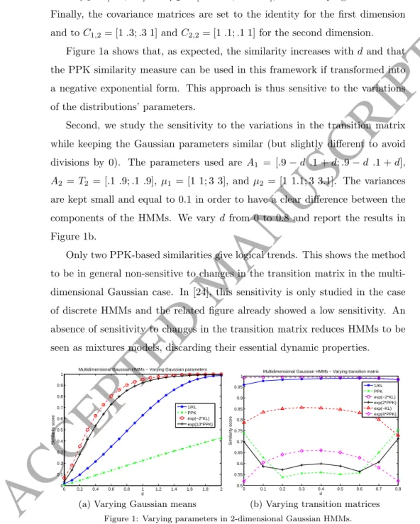
Finally, the covariance matrices are set to the identity for the first dimension and toC1,2= [1.3;.3 1] andC2,2= [1.1;.1 1] for the second dimension.
Figure 1a shows that, as expected, the similarity increases withdand that the PPK similarity measure can be used in this framework if transformed into a negative exponential form. This approach is thus sensitive to the variations of the distributions’ parameters.
Second, we study the sensitivity to the variations in the transition matrix while keeping the Gaussian parameters similar (but slightly different to avoid divisions by 0). The parameters used are A1 = [.9−d .1 +d;.9−d .1 +d],
A2 =T2 = [.1 .9;.1.9], µ1 = [1 1; 3 3], andµ2 = [1 1.1; 3 3.1]. The variances
are kept small and equal to 0.1 in order to have a clear difference between the components of the HMMs. We vary dfrom 0 to 0.8 and report the results in Figure 1b.
Only two PPK-based similarities give logical trends. This shows the method to be in general non-sensitive to changes in the transition matrix in the multi-dimensional Gaussian case. In [24], this sensitivity is only studied in the case of discrete HMMs and the related figure already showed a low sensitivity. An absence of sensitivity to changes in the transition matrix reduces HMMs to be seen as mixtures models, discarding their essential dynamic properties.
0 0.2 0.4 0.6 0.8 1 1.2 1.4 1.6 1.8 2 0 0.1 0.2 0.3 0.4 0.5 0.6 0.7 0.8 0.9 1 d Similarity score
Multidimensional Gaussian HMMs − Varying Gaussian parameters
1/KL PPK exp(−2*KL) exp(10*PPK)
(a) Varying Gaussian means
0 0.1 0.2 0.3 0.4 0.5 0.6 0.7 0.8 0.5 0.55 0.6 0.65 0.7 0.75 0.8 0.85 0.9 0.95 1 d Similarity score
Multidimensional Gaussian HMMs − Varying transition matrix
1/KL PPK exp(−2*KL) exp(2*PPK) exp(−KL) exp(4*PPK)
(b) Varying transition matrices
Figure 1: Varying parameters in 2-dimensional Gaussian HMMs.
dis-ACCEPTED MANUSCRIPT
tances by making it vary from 1 to 20 for the exponential forms of the approach (using the same parameters as the ones used for Figure 1a). The results, in Figure 2, pinpoint a major flaw of the approach. The final similarity measure drastically varies, making the results non objective unless under a careful study of this coefficient’s tuning.
0 0.2 0.4 0.6 0.8 1 1.2 1.4 1.6 1.8 2 0 0.1 0.2 0.3 0.4 0.5 0.6 0.7 0.8 0.9 1 d Similarity score
Influence of coefficient k − Gaussian HMMs
Figure 2: Varyingκwith 2-dimensional Gaussian HMMs. Plain curves for PPK-based simi-larity and dashed curves for KL-based similarities.κvaries from 1 to 10,κ= 1 for the lowest curve of each network of curves.
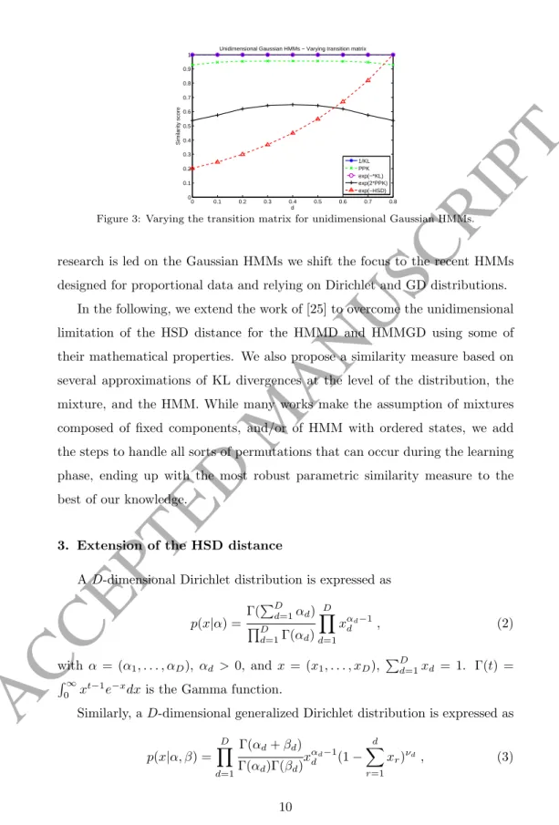
With these results in mind, we study how the HSD approach [25] behaves compared to the previously tested methods. As already said, its main limita-tion resides in the fact that it only applies to unidimensional distribulimita-tions. Its efficiency giving coherent distances when the Gaussian parameters are changed is clearly illustrated in the original paper and we only present the results for variations in the transition matrix. The parameters used areA1= [.9−d .1 +
d;.9−d .1 +d], A2 = T2, µ1 = µ2 = [1; 3], and the variances equal to 0.10
and 0.11. Here and in all subsequent graphs, we plot the HSD distance ∆ as a similarity score by computingexp(−∆), in order to be able to compare with the other approaches. In Figure 3, the HSD metric perfectly grasps the variations imposed to the transition matrix and, once again, the approach of [24], with whatever inner distance setting, does not achieve to grasp these variations.
These results clearly show the need of designing new distances for multidi-mensional continuous HMMs that exhibit a sensitivity in changes of the distri-bution parameters, of the transition matrix, and of the mixing matrix. As most
ACCEPTED MANUSCRIPT
0 0.1 0.2 0.3 0.4 0.5 0.6 0.7 0.8 0 0.1 0.2 0.3 0.4 0.5 0.6 0.7 0.8 0.9 1 d Similarity scoreUnidimensional Gaussian HMMs − Varying transition matrix
1/KL PPK exp(−*KL) exp(2*PPK) exp(−HSD)
Figure 3: Varying the transition matrix for unidimensional Gaussian HMMs.
research is led on the Gaussian HMMs we shift the focus to the recent HMMs designed for proportional data and relying on Dirichlet and GD distributions.
In the following, we extend the work of [25] to overcome the unidimensional limitation of the HSD distance for the HMMD and HMMGD using some of their mathematical properties. We also propose a similarity measure based on several approximations of KL divergences at the level of the distribution, the mixture, and the HMM. While many works make the assumption of mixtures composed of fixed components, and/or of HMM with ordered states, we add the steps to handle all sorts of permutations that can occur during the learning phase, ending up with the most robust parametric similarity measure to the best of our knowledge.
3. Extension of the HSD distance
AD-dimensional Dirichlet distribution is expressed as p(x|α) = Γ( PD d=1αd) QD d=1Γ(αd) D Y d=1 xαd−1 d , (2) with α = (α1, . . . , αD), αd > 0, and x = (x1, . . . , xD), PDd=1xd = 1. Γ(t) = R∞
0 xt−1e−xdxis the Gamma function.
Similarly, aD-dimensional generalized Dirichlet distribution is expressed as p(x|α, β) = D Y d=1 Γ(αd+βd) Γ(αd)Γ(βd)x αd−1 d (1− d X r=1 xr)νd , (3)
ACCEPTED MANUSCRIPT
withα= (α1, . . . , αD),αd>0,β = (β1, . . . , βD),βd>0, andx= (x1, . . . , xD), PD
d=1xd<1. νdis defined asνd=βd−αd+1−βd+1ifd6=DandνD=βD−1.
The limitation of the HSD distance to unidimensional distributions is due to the fact it relies on the computation of the cumulative distribution function (CDF) of the distributions composing the HMM. The concept of CDF is un-defined for multidimensional distributions, hence the distance cannot apply to them. However, the GD distribution has the following property [30, 31]:
Property 1: A D-dimensional generalized Dirichlet,GD(α1, ..., αD, β1, ..., βD),
is equivalent to a set of D independent Beta distributions with the same pa-rameters (αn, βn), n= 1, . . . , D, in a particular transformed data space that is
reached through a bijection. The bijective function linking the two data spaces is expressed asW={Wn}1:Dwith: Wn= xn, forn= 1, xn 1−Pni=1−1xi , forn∈[2, D]. (4)
Beta distributions, are unidimensional by definition and their CDF is easily computable. We can then make up a simple function that acts as an equivalent of the CDF for multidimensional generalized Dirichlet distributions and keep the rest of the distance computation untouched.
When working with the Dirichlet distribution, another transform is first required to express it into a generalized Dirichlet form. Indeed, the Dirichlet is a degenerate case of generalized Dirichlet [31].
Property 2: AD-dimensional generalized DirichletGD(α1, ..., αD, β1, ..., βD),
which parameters verifyβn=αn+1+βn+1, forn= 1, . . . ,(D−1), is a Dirichlet
distribution with parametersDir(α1, . . . , αD, βD).
Reversing this expression allows to express a Dirichlet distribution in the form of a generalized Dirichlet one and thus to apply an extended form of the HSD distance computation to it.
In summary, Beta distributions are used to characterize the HMM in a trans-formed data space and the HSD measure can be deployed using them. The
ACCEPTED MANUSCRIPT
resulting distance is equivalent to the distance that could have been computed in the initial space as these two spaces are connected through a bijection.
The computation of the HSD distance for multidimensional Dirichlet and GD distribution-based HMMs follows the steps:
1. For each state of each HMM, express the Dirichlet distributions in their GD form [31]: Dir(α1, ..., αD+1)≡GD(α1, ..., αD, β1, ..., βD), withβj =
αj+1+βj+1forj= 1, . . . ,(D−1) andβD=αD+1
2. Initialize the distance ∆ and the valuexto 0, and the step size tos= 1/L (hereafter,L= 100)
3. Iteratively doLtimes the following steps:
(a) For each statek, dimensiond, and HMMsi= 1,2, compute BetaCDFi,k,d(αi,k,d, βi,k,d, x)
(b) For each statekof each HMMi, compute CDFi,k=PDd=1BetaCDFi,k,d
(c) Compute the models’ CDFs using a dot product Fi=hΠs,i,CDFii
(d) Compute ∆ = ∆ +s× |F1(x)−F2(x)|
(e) Incrementxbys
When the models are based on GD distributions, the first step is obviously omitted. Experimental results for this distance are reported in Section 6.
4. Parametric KL-divergence for HMMD and HMMGD
We propose to derive a parametric similarity measure for HMMD and HM-MGD under the assumption that mixtures are indivisible elements. This means that either these mixtures have some physical representation and that their components cannot be split up over different states, or that the components found while initializing the HMM have been ordered following some heuristic rules. The computation of this similarity measure needs to take into account the potential permutation of the mixtures over the different states. The measure is first derived as a KL divergence, and converted into a similarity measure at the very last step.
ACCEPTED MANUSCRIPT
As we intend to compute a parameter-based metric similar in behavior to the KL divergence, we start from its definition for two functionsf1 andf2:
D(f1||f2) = Z f1ln f 1 f2 . (5)
When data samplesX={x1, . . . , xT}are available, a Monte-Carlo
approx-imation of Equation (5) gives: D(f1||f2)≈ 1 T T X t=1 (ln(f1(xt))−ln(f2(xt))). (6)
For this approximation to be accurate,T needs to be large enough. In the case of HMMs,f1andf2can be identified as the likelihood of the data with respect
to the HMMsλ1andλ2, respectively. AsT increases, the computation of these
quantities becomes heavier and at some point, even prohibitive2.
[20] devised a method to approximate an upper bound to the KL divergence for Dependence Trees and showed that it can be used for left-to-right HMMs, which can be considered as a special case of dependence trees. Using the pro-posed approximation, we write:
D(λ1||λ2)≤ K X k=1
πk01(D(aj||˜aj) +D(bj||˜bj)), (7)
whereπ0 is the stationary distribution ofλ1. The stationary distribution of an
HMM is iteratively computed as proposed in [25], starting from the initial state pmfπ0
0=πand following the recursive equation:
πt+10 =π0tA . (8)
Using Equation (7) implies that the distance does not take into account the transitional phase of the HMM. However, our experiments show that even
2The computation of this quantity requires the sampling of data generated by the HMM
and the use of the forward-backward algorithm. Both have a complexity linear inT. The computation needs to be repeated several times for accounting for the non-deterministic nature of the distance and for reducing the variance. Moreover, for Dirichlet and GD-based models, explosions of gradients in the forward-backward algorithm have been observed when sequences become too long [7].
ACCEPTED MANUSCRIPT
for HMMs trained on short sequences, the similarity measure we are deriving behaves as expected and gives good discriminative results (see Section 6).
As a side note, the only experiments carried out in [20] use a simple dis-crete HMM (with pre-defined parameters), two states and tri-dimensional data. Therefore, more extensive experiments with a similarly designed method are needed to assess the potential discriminative performance of such parameter-based approximation of the KL divergence.
In Equation (7), the term D(aj||˜aj) refers to the rows of the transition
matrices. Each row of a transition matrix is a probability mass function and therefore the KL divergence can be easily computed. However, given that HMMs do not have in general a left-to-right topology, we first need to pair up the states of the two models. We propose to see this task as a linear assignment problem and solve it using the Jonker-Volgenant algorithm [32], which provides a faster implementation than the well-known Hungarian algorithm. The Jonker-Volgenant algorithm provides a cost matrix for pairing up each state ofλ1with
each state ofλ2, as well as the sequence of pairs that minimizes the assignment
cost. From this sequence of pairs, we build a permutation matrixR=ri,j, where
ri,j = 1 if statei ofλ1 is optimally matched to statej ofλ2 and 0 otherwise.
The transition matrix of the HMM λ2 is then permuted as ˜A0 = RA˜R. The
mixtures assigned to each state are permuted accordingly.
The second term of Equation (7),D(bj||˜bj) refers to the emission probability
distributions assigned to each state which are, in our case, mixtures. The KL divergence of mixture models does not have a closed form expression and then requires to be approximated. Hershey and Olsen [33] proposed a full review of techniques to approximate the KL divergence between two mixtures of Gaussian. Studying the assumptions made, most of the approximations they proposed can be applied to mixtures of Dirichlet and generalized Dirichlet without restriction. The variational approximation they proposed is chosen here for the good results it showed for the Gaussian case in [33], especially as the criterion used in that study is the similarity to the classic data-based KL divergence estimation, which is also one of our criterion for the design of this HMM distance.
ACCEPTED MANUSCRIPT
Denoting the mixtures asP1=PMm=1w1,mp1,mand P2=PMm=1w2,mp2,m,
the variational approximation is written as:
D(P1||P2) = M X m=1 w1,m PM a=1w1,ae−D(p1,m||p1,a) PM b=1w2,be−D(p1,m||p2,b) . (9)
Equation (9) requires the computation of the KL divergence between two Dirichlet (and GD) distributions. The KL divergence between two D-dimensional Dirichlet distributionsDir1(α~1) andDir2(~α2) can be expressed as:
KL(Dir1||Dir2) = ln(Γ( D X d=1 α1,d))− D X d=1 ln(Γ(α1,d))−ln(Γ( D X d=1 α2,d)) + D X d=1 ln(Γ(α2,d)) + D X d=1 (α1,d−α2,d)Ψ(α1,d−Ψ( D X j=1 α1,j)). (10) Similarly, the KL divergence between two D-dimensional generalized Dirich-let distributionsGD1(~α1, ~β1) andGD2(~α2, ~β2) is expressed as [34]:
KL(GD1||GD2) = D X d=1 ln Γ(α1,d+β1,d) Γ(α1,d)Γ(β1,d) Γ(α2,d)Γ(β2,d) Γ(α2,d+β2,d) ! − D X d=1 (α1,d−α2,d) Ψ(α1,d)−Ψ(β1,d)− d X s=1 (Ψ(α1,s+β1,s) −Ψ(β1,s)) ! + D X d=1 (ν1,d−ν2,d) d X s=1 (Ψ(α1,s+β1,s)−Ψ(β1,s)). (11) The steps of the KL divergences computation are given in Appendices A and B. The set of Equations (7) to (11), allows to compute a measure between two HMMD or HMMGD without the need to generate data of any kind. This measure can be made symmetric usingD(λ1, λ2) = (D(λ1||λ2) +D(λ2||λ1))/2
and transformed into a similarity measure by taking the inverse exponential S=e−D(λ1,λ2). In Section 6, we show how well this similarity measure performs
on HMMs with randomly generated parameters, even when the HMM states are permuted. Some sets of equations for training an HMM do not impose
ACCEPTED MANUSCRIPT
any constraint upon how the initial mixture components found in the data are assigned to the states [17]. In that case, the sole assumption of state permutation is not strong enough. Therefore, there is a need to design a simple method allowing for component permutation between mixture models. Such a method is presented in the next section.
5. Extension of the proposed distance
HMMs based on mixtures of Dirichlet have been first introduced in [17] and the ones based on generalized Dirichlet in [28] and [7]. The learning process requires initial values for all HMMs parameters, including the emission distri-butions. This initialization is based on a simple k-means clustering followed by a moment matching procedure. The estimated distributions are then grouped into mixtures depending on the chosen values forK andM. The k-means clustering has no constraint on the choice of the seeds, so does the grouping procedure and therefore, in general, HMMs trained from the same data will have different mixtures (i.e., mixtures composed of different components) assigned to different states. These HMMs are yet totally equivalent and will perform the same way, with equivalent accuracies in classification tasks.
In these cases, the approach devised in the previous section does not make sense as one of the assumptions made is not respected. In order to take into account all the possible permutations, another quantity needs to be defined that allows to find a distance measure close to 0 when HMMs are equivalent (or similarity close to 1) even if their parameters, at first look, are different. The
natural KL divergence achieves it by looking at the likelihood values directly. In order to devise a new relevant quantity, we get inspired by the initial-ization process of the HMM learning algorithm as proposed in [7] that relies of a k-means clustering amongK∗M clusters. As the subsequent grouping of components into mixture models impacts the values of the transition matrix, of the mixing matrix, and of the initial state probability mass function, we cannot rely on these parameters as is. In order to see how close two HMMs are, we
ACCEPTED MANUSCRIPT
need to somehow revert this process i.e., combine these parameters in order to
decorrelate them from the mixture models. The procedure can be illustrated with this question: What is the closest equivalent as a non-mixture HMM that we can get from a mixture-based HMM? Obviously this will be a loose equiva-lence and in no case a bijection. However, we propose here a quantity that we call theflatten transition matrixthat is simple and efficient enough to compute discriminative distances as we show later on simple illustrations using real-world data in Section 7.
Building theflatten transition matrixA0. - This quantity reflects what the tran-sition matrix of aK-state mixture-based HMM with mixture ofM components
flatteninto a non-mixture HMM withK∗Mcomponent would be equivalent to. This approximation naturally depends on the transition matrixA={aij}K×K
and the mixing matrixC = {cij}K×M of the HMM. Given that we work
un-der the assumption of stationary HMM, the initial state probability π is not involved. Theflatten transition matrix is expressed as:
A0= a11c11 ... a11c1M a12c21 ... a1KcK1 ... a1KcKM
repeat over (M-2) rows
a11c11 ... a11c1M a12c21 ... a1KcK1 ... aK1cKM
a21c11 ... a21c1M a22c21 ... a2KcK1 ... a2KcKM
repeat over (M-2) rows
a21c11 ... a21c1M a22c21 ... a2KcK1 ... a2KcKM .. . .. . aK1c11 ... aK1c1M aK2c21 ... aKKcK1 ... aKKcKM
repeat over (M-2) rows
aK1c11 ... aK1c1M aK2c21 ... aKKcK1 ... aKKcKM . (12)
The repetition of lines is due to the fact the transition matrix of mixtures-based HMMs only depends on the previous hidden state and not of the mixture com-ponent by which the observation is actually modeled. Therefore, even though we keep a squareKM×KM matrix to match the shape of an HMM transition
ACCEPTED MANUSCRIPT
matrix, there are actually onlyK2M different coefficients. All the rows sum up
to one and thusA0 is a valid transition matrix. There is no need for a mixing matrix C0 as no mixture are then involved, and an extended π0 initial pmf is computed as follows:
π0= (π11c11, . . . , π11c1M, π12c21, . . . , π1KcK1, . . . , π1KcKM) (13)
We now approximated a non-mixture HMM from the original HMM. The single distributions (mixture components) are assigned accordingly to the wayA0 is constructed. The approach devised in the previous section can be used with HMMs flatten this way, by directly applying the linear assignment matching algorithm at the component level (which are now the states of theflattenversion of the HMM).
One can note that the equations used to derive the proposed measure can be applied to any HMM with or without mixtures and based on the Beta, Dirichlet, or generalized Dirichlet distributions. It can also be generalized to any distribution for which the KL-divergence can be computed or approximated.
6. Comparative study over synthetic data
In order to lead a comparative study of the different metrics, we lead sev-eral series of experiments over randomly generated HMMs, making each set of parameters vary independently from the others. The quantification of the performance of the different similarity measures tested requires the definition of quantities that are meaningful for this purpose. Indeed, when working in a space where nonatural physical distance exist but only artificially designed ones, which reference to use to compare how well is a distance doing? It mostly depends on the expectations of the person who uses it. For this reason, the behavior of the distance has to be characterized under different aspects.
We propose to compute the following quantities:
• The correlation to the parameters average variation which quantifies how close the variations of the measure and the individual parameters are.
ACCEPTED MANUSCRIPT
• The autocorrelation at lag 1 for a continuous variation of the parameters which quantifies the smoothness of the measure with respect to the evo-lution of the parameters. In the case of two models whose parameters continuously go further away, a coefficient close to 1 means a very smooth function, -1 means that the function is irregular/non-monotonic which is not desirable.
• The average variation by unitary variation (for a variation of parameterd equal to 1) of the parameters which quantifies of how discriminative the measure is.
• The correlation to the KL divergence computed from generated data which illustrates how the behavior of the parameter-based measures is compared to the reference data-based one, especially in term of stability.
• The average distance to the KL divergence computed from generated data which illustrates how the behavior of the parameter-based measures is compared to the reference data-based one, especially in terms of discrim-inability.
Among them, one has to note that the data-based KL divergence has some limitations exhibited in [24]and in the experiments presented hereafter. How-ever, we compute how close the tested distances are to the KL divergence as it is usually taken as the reference for HMMs and generative models in gen-eral [35, 23, 36]. When the correlation of the data-based KL divergence to the parameters variation is not strong, points 4 and 5 are obviously not relevant anymore. Therefore, points 1 to 3 are found to be the more reliable way of comparing similarity measures.
Some of the compared works define distances, in which case the inverse exponential of the distance is used as a similarity measure. The data-based KL divergence is computed by generating a sequence of data of lengthT = 100 from the reference HMM.
uni-ACCEPTED MANUSCRIPT
form distributions with Dirichlet and GD parameters in the range [0,20]. There-fore, the presented results are penalized by some occurrences or low discrim-inability between some components that do not occur in real scenarios (as the initial clustering would create a unique cluster for samples following this distri-bution). The HMM parameters are fixed toK = 5,M = 2,D= 4, these values are small enough to keep the component similarities occurrences low, and big enough to have some of the measures failing. In the following experiments, the sensitivity of the measures to the variation of each type of parameter is studied separately for a clear illustration of the strength and weaknesses of each of them.
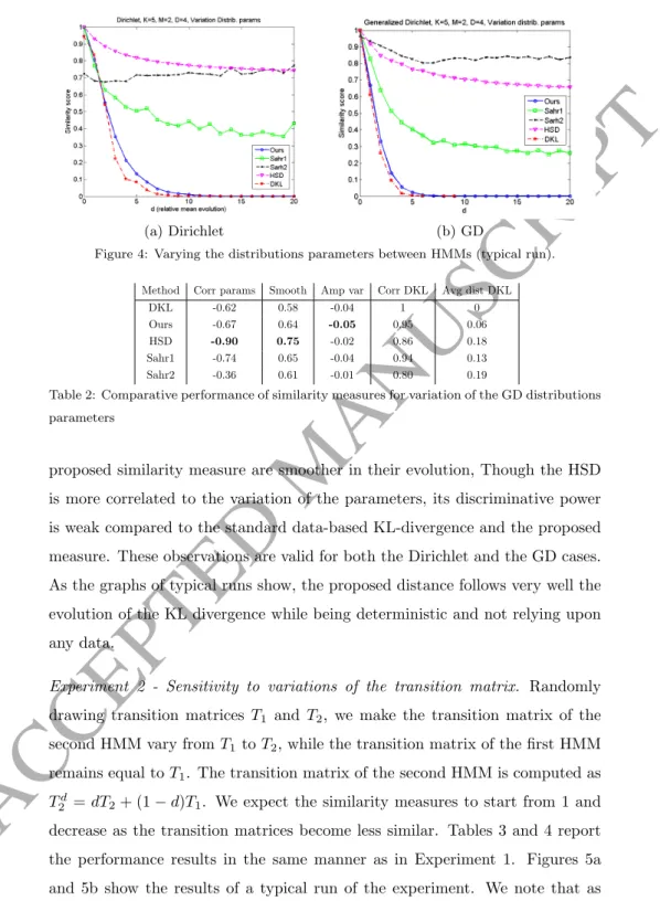
Experiment 1 - Sensitivity to variations of the distribution parameters. The parameters of the Dirichlet/GD distributions of one of the HMMs are varied by adding a constantdbetween 0 and 20 to the concentration parameters. We expect the similarity measures to start from 1 and rapidly decrease to 0 as the parameters variation is quite important, and the analysis, exponential. Tables 1 and 2 report the performance results of the approaches of [24], the proposed extension of the HSD distance, the data-based Kullback-Leibler divergence, and the proposed distance. Figures 4a and 4b show the results of a typical run of the experiment (each set of experiments is repeated 20 times at least).3
Method Corr params Smooth Amp var Corr DKL Avg dist DKL
DKL -0.70 0.68 -0.05 1 0
Ours -0.75 0.72 -0.05 0.99 0.06
HSD -0.86 0.72 -0.01 0.95 0.19
Sahr1 -0.74 0.66 -0.04 0.97 0.12
Sahr2 -0.08 0.64 ≤-0.01 0.48 0.17
Table 1: Comparative performance of similarity measures for variation of the Dirichlet distri-butions parameters
Besides theSahr2 similarity measure, all similarity measures are sensitive to distributions parameters variations. However, the extended HSD and the
3For all experiments the labels have to be read as follow: DKL is the data-based KL
divergence. Sahr1 and Sahr2 are the methods of [24] with similarities computed as the inverse of the distance and the inverse exponential, respectively. HSDis the extended HSD distance presented in Section 3.Oursis the method proposed in Section 4.
ACCEPTED MANUSCRIPT
(a) Dirichlet (b) GD
Figure 4: Varying the distributions parameters between HMMs (typical run).
Method Corr params Smooth Amp var Corr DKL Avg dist DKL
DKL -0.62 0.58 -0.04 1 0
Ours -0.67 0.64 -0.05 0.95 0.06
HSD -0.90 0.75 -0.02 0.86 0.18
Sahr1 -0.74 0.65 -0.04 0.94 0.13
Sahr2 -0.36 0.61 -0.01 0.80 0.19
Table 2: Comparative performance of similarity measures for variation of the GD distributions parameters
proposed similarity measure are smoother in their evolution, Though the HSD is more correlated to the variation of the parameters, its discriminative power is weak compared to the standard data-based KL-divergence and the proposed measure. These observations are valid for both the Dirichlet and the GD cases. As the graphs of typical runs show, the proposed distance follows very well the evolution of the KL divergence while being deterministic and not relying upon any data.
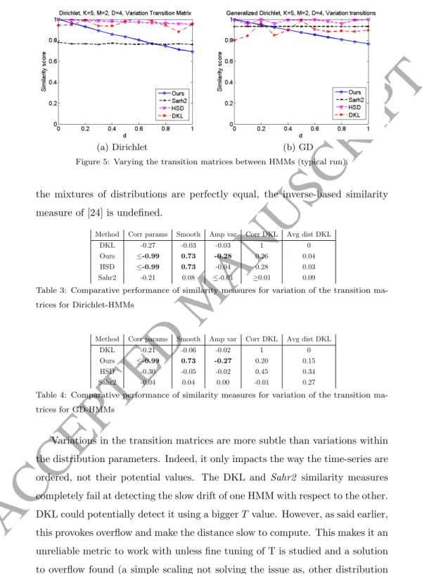
Experiment 2 - Sensitivity to variations of the transition matrix. Randomly drawing transition matrices T1 and T2, we make the transition matrix of the
second HMM vary fromT1toT2, while the transition matrix of the first HMM
remains equal toT1. The transition matrix of the second HMM is computed as
Td
2 =dT2+ (1−d)T1. We expect the similarity measures to start from 1 and
decrease as the transition matrices become less similar. Tables 3 and 4 report the performance results in the same manner as in Experiment 1. Figures 5a and 5b show the results of a typical run of the experiment. We note that as
ACCEPTED MANUSCRIPT
(a) Dirichlet (b) GD
Figure 5: Varying the transition matrices between HMMs (typical run).
the mixtures of distributions are perfectly equal, the inverse-based similarity measure of [24] is undefined.
Method Corr params Smooth Amp var Corr DKL Avg dist DKL
DKL -0.27 -0.03 -0.03 1 0
Ours ≤-0.99 0.73 -0.28 0.26 0.04
HSD ≤-0.99 0.73 -0.04 0.28 0.03
Sahr2 -0.21 0.08 ≤-0.01 ≥0.01 0.09
Table 3: Comparative performance of similarity measures for variation of the transition ma-trices for Dirichlet-HMMs
Method Corr params Smooth Amp var Corr DKL Avg dist DKL
DKL -0.21 -0.06 -0.02 1 0
Ours ≤-0.99 0.73 -0.27 0.20 0.15
HSD -0.30 -0.05 -0.02 0.45 0.34
Sahr2 -0.04 0.04 0.00 -0.01 0.27
Table 4: Comparative performance of similarity measures for variation of the transition ma-trices for GD-HMMs
Variations in the transition matrices are more subtle than variations within the distribution parameters. Indeed, it only impacts the way the time-series are ordered, not their potential values. The DKL and Sahr2 similarity measures completely fail at detecting the slow drift of one HMM with respect to the other. DKL could potentially detect it using a biggerT value. However, as said earlier, this provokes overflow and make the distance slow to compute. This makes it an unreliable metric to work with unless fine tuning of T is studied and a solution to overflow found (a simple scaling not solving the issue as, other distribution
ACCEPTED MANUSCRIPT
(a) Dirichlet (b) GD
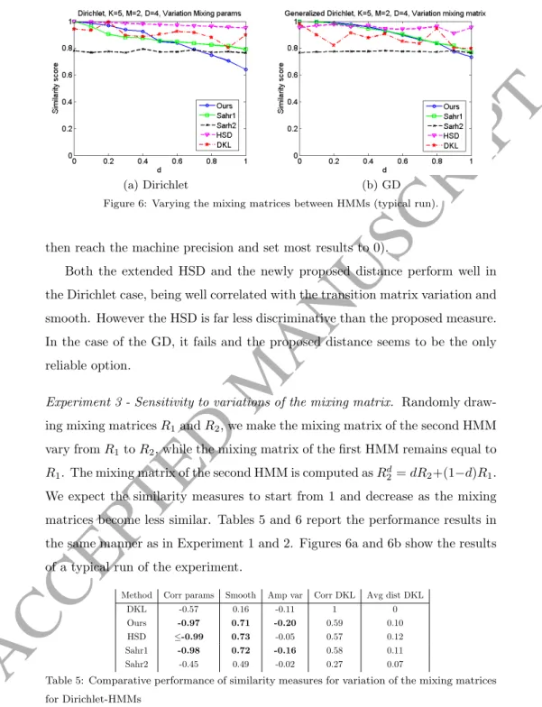
Figure 6: Varying the mixing matrices between HMMs (typical run).
then reach the machine precision and set most results to 0).
Both the extended HSD and the newly proposed distance perform well in the Dirichlet case, being well correlated with the transition matrix variation and smooth. However the HSD is far less discriminative than the proposed measure. In the case of the GD, it fails and the proposed distance seems to be the only reliable option.
Experiment 3 - Sensitivity to variations of the mixing matrix. Randomly draw-ing mixdraw-ing matricesR1andR2, we make the mixing matrix of the second HMM
vary fromR1toR2, while the mixing matrix of the first HMM remains equal to
R1. The mixing matrix of the second HMM is computed asRd2=dR2+(1−d)R1.
We expect the similarity measures to start from 1 and decrease as the mixing matrices become less similar. Tables 5 and 6 report the performance results in the same manner as in Experiment 1 and 2. Figures 6a and 6b show the results of a typical run of the experiment.
Method Corr params Smooth Amp var Corr DKL Avg dist DKL
DKL -0.57 0.16 -0.11 1 0
Ours -0.97 0.71 -0.20 0.59 0.10
HSD ≤-0.99 0.73 -0.05 0.57 0.12
Sahr1 -0.98 0.72 -0.16 0.58 0.11
Sahr2 -0.45 0.49 -0.02 0.27 0.07
Table 5: Comparative performance of similarity measures for variation of the mixing matrices for Dirichlet-HMMs
ACCEPTED MANUSCRIPT
Method Corr params Smooth Amp var Corr DKL Avg dist DKL
DKL -0.55 0.18 -0.23 1 0
Ours -0.97 0.71 -0.27 0.57 0.13
HSD -0.64 0.19 -0.05 0.69 0.14
Sahr1 -0.98 0.72 -0.14 0.59 0.14
Sahr2 -0.43 0.51 -0.01 0.35 0.48
Table 6: Comparative performance of similarity measures for variation of the mixing matrices for GD-HMMs
Variations of the mixing coefficients have a similar action on the generated data as a variation of the transition coefficients: it only impacts the way the time-series are ordered but not their values. It is therefore not surprising to see that the proposed approach allows good discrimination, good smoothness, and good correlation with the variation of the mixing coefficients. The extended HSD approach is valid here again in the Dirichlet case only but with a weak discriminative potential. TheSahr1 similarity measure works surprisingly well with just a bit less discriminative power than our proposed approach. However, it still relies on the tuning of theκparameter which is not straightforward.
Overall, only the proposed approach shows itself successful to detect and log-ically reflect any kind of variation in the HMM model based on either Dirichlet or generalized Dirichlet, without requiring any data not any parameter tuning. The proposed extension of the HSD also reflects well the changes for Dirichlet-based HMMs but does not perform equally in the generalized Dirichlet case when the transition of mixing coefficients vary. Its discriminative power is lower which can also be the reason why it cannot achieve good performance when
minor parameters of the HMMs vary. The discriminative power of this mea-sure could be enhanced by adding a multiplicative coefficient when computing the approximate CDF while making the distance performance dependent of the tuning of that new parameter.
Beyond the actual performance results, this study over synthetic data clearly shows that the similarity measures we test our methods against were lacking some performance criteria. The proposed criteria address a range of character-istics: correlation to the variation of the parameters, smoothness of the function,
ACCEPTED MANUSCRIPT
and discriminative power. These criteria are simple enough to be easily com-puted and powerful enough to show the limitations of all the state-of-the-art method for parametric distances between mixture-based HMMs.
7. Illustration with real data
The extension of the method, as presented in Section 5 is valid for HMMs that are trained as described in [17] and [7], using a component by component, k-means based initialization. As no bijective transformation is known between mixture-based HMMs, experiments validating our approach for the case when all components are assigned to different states are not possible with synthetic data.
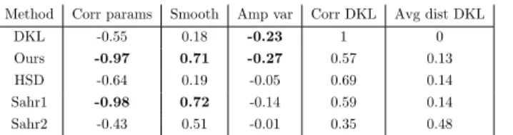
We present hereafter, some illustrations of use of this metric through cluster-ing operations. A main constraint for clearly illustratcluster-ing the proposed measure behavior is that, HMMs seldom represent something concrete that is itself mea-surable by a distance. Indeed, HMMs are most of the time trained over abstract features extracted from some data, and once trained provide a very high-level representation of these data. Images appear to be a good way of getting some visual assessment of the performance. Therefore, we study the behavior of the designed similarity measure with respect to HMMs trained over the UCSD Ped1 and Ped2 data sets [37] and over a sea surveillance footage [38], following the method presented in [7]. The video sequences of the data sets are divided into 3D volumes. As the camera capturing the sequence is still, each volume rep-resent a fixed spatial area of the camera field i.e., grass, trees, walkway with pedestrians, sea, pier, sky. An HMM is trained over each 3D volume location thus, we expect our designed metric to show high similarity between HMMs trained at locations with similar content (e.g., volumes representing trees) and lower similarity between HMMs representing volumes featuring trees versus the walkway for example. In this application we haveK = 3,M = 2, andD= 12 and use spatio-temporal gradient-based features. We refer the interested reader to [7] for the details of the approach.
ACCEPTED MANUSCRIPT
Working with real-data requires a few adjustments. First of all, for the Dirichlet case, the parameters resulting from a training algorithm are often-times very high because of the variance which is badly estimated. In order to counter this artifact involved by some training methods, we use the mean of the Dirichlet (which is the normalized concentration vector) and rescale it in the range [0,20].4
After dividing the frame space into 77 overlapping patches (50% overlap) and training one HMM per location, we propose to compute the similarities between these HMMs (building a 77x77 similarity matrix) to unravel major patterns in the frames.
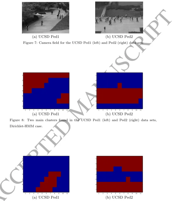
7.1. Hierarchical clustering over the UCSD data sets
We apply hierarchical clustering using our proposed similarity measure over the UCSD data sets. The camera field for these data sets are reported in Figure 7. We expect to find two clusters, one across the walkway, and one across the vegetation. This is a reasonable expectation as the spatio-temporal features used for the training take into account both the appearance and the dynamics of the scene, and that pedestrians only walk on the walkway in the training video sequences. We report hereafter in Figures 8 and 9, the 2 main clusters found across the trained Dirichlet and generalized Dirichlet HMMs, respectively.
The proposed similarity measure allows the clustering of the two main zones of the camera field, the walkway versus the trees and grass where no dynamic action takes place for both Dirichlet and GD-based HMMs. We can see that the clustering results are somehow different on Ped1 but still make sense as
4There is no risk of confusion with potential estimation of Dirichlet with parameters below
1, as Dirichlet distribution with such parameters exhibit several peaks on the ”border” of the space they belong instead of a unique strong peak. The initial clustering performed for initializing the HMM naturally prevents this case to happen, as a distribution exhibiting two peaks would rather by approximate by two distributions with one peak each (minimizing the intra-class variance).
ACCEPTED MANUSCRIPT
(a) UCSD Ped1 (b) UCSD Ped2
Figure 7: Camera field for the UCSD Ped1 (left) and Ped2 (right) data sets
1 2 3 4 5 6 7 8 9 10 11 1 2 3 4 5 6 7
(a) UCSD Ped1
1 2 3 4 5 6 7 8 9 10 11 1 2 3 4 5 6 7 (b) UCSD Ped2
Figure 8: Two main clusters found in the UCSD Ped1 (left) and Ped2 (right) data sets, Dirichlet-HMM case. 1 2 3 4 5 6 7 8 9 10 11 1 2 3 4 5 6 7
(a) UCSD Ped1
1 2 3 4 5 6 7 8 9 10 11 1 2 3 4 5 6 7 (b) UCSD Ped2
Figure 9: Two main clusters found in the UCSD Ped1 (left) and Ped2 (right) data sets, GD-HMM case.
ACCEPTED MANUSCRIPT
(a) Sample frame
1 2 3 4 5 6 7 8 9 10 11 1 2 3 4 5 6 7 (b) Dirichlet 1 2 3 4 5 6 7 8 9 10 11 1 2 3 4 5 6 7 (c) GD
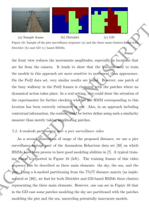
Figure 10: Sample of the pier surveillance sequence (a) and the three main clusters found with Dirichlet (b) and GD (c) based HMMs.
the front view reduces the movements amplitudes, especially in locations that are far from the camera. It tends to show that the features used to train the models in this approach are more sensitive to movement than appearance. On the Ped2 data set, very similar results are found. However, one patch of the busy walkway in the Ped2 frames is clustered with the patches where no dynamical action takes place. In a real setting, this could draw the attention of the experimenter for further checking whether the HMM corresponding to this location has been correctly estimated or not. Also, in an approach including contextual information, the context could be better define using such a similarity measure than merely taking neighboring patches.
7.2. k-medoids partitioning over a pier surveillance video
As a second illustration of usage of the proposed distance, we use a pier surveillance footage part of the Anomalous Behaviour data set [38] on which HMMs have been proven to have good modeling abilities in [7]. A typical train-ing frame is reported in Figure 10 (left). The traintrain-ing frames of this video sequence can be described as three main elements: the sky, the sea, and the pier. Using a k-medoid partitioning from the 77x77 distance matrix (as imple-mented at [39]), we find for both Dirichlet and GD-based HMMs three clusters representing the three main elements. However, one can see in Figure 10 that in the GD case some patches modeling the sky are partitioned with the patches modeling the pier and the sea, unraveling potentially inaccurate models.
ACCEPTED MANUSCRIPT
8. Conclusion
We proposed the first parametric similarity measures for the recently pro-posed Dirichlet and generalized Dirichlet-based HMMs (and by extension, Beta-based). We overcame the main limitation of the HSD distance proposed in [25] by extending it to the multidimensional case. Though behaving as expected for variations in the distributions and transition parameters, it failed at detect-ing changes in the mixdetect-ing matrix. The new approach we proposed, showed a great ability to detect any change in any of the HMM parameters, with good discriminative ability and without requiring any data. Its good correlation to parameters’ variations as well as its smoothness makes it a distance of choice for these models. The extensive experiments carried out over synthetic data as well as the practical comparative performance for 5 similarity measures allows one to knowingly choose right metric for their case of study. The extension of the proposed distance to models trained by component, illustrated with real-data, showed coherent results and exemplified how one can explore the HMM data representation in order to detect erroneous models or to refine the concept of neighbor in some approaches that use contextual information.
Acknowledgment
The completion of this research was made possible thanks to the Natural Sciences and Engineering Research Council of Canada (NSERC).
Appendix A. Appendix: KL divergence between two Dirichlet dis-tributions
Hereafter are shown the steps to derive the KL divergence between two multidimensional Dirichlet distributions. We use the usual notation KL(p||q) for the divergence between a distributionpand another distributionq.
ACCEPTED MANUSCRIPT
We denote p(x|α) andq(x|a) as two D-dimensional Dirichlet distributions as defined in Equation (2) and derive the following quantity
KLdir(p||q) = Z p(x) ln p(x) q(x) dx . (A.1)
We typically recognize the expression of an expectation with respect to p and introduce the following notation for it
KLdir(p||q) = ln p(x) q(x) p(x) =hln(p(x))−ln(q(x))ip(x). (A.2)
Using Equations (2) and (A.2), we get KLdir(p||q) = ln Γ XD d=1 αd − D X d=1 ln(Γ(αd)) −ln Γ XD d=1 ad + D X d=1 ln(Γ(ad)) + D X d=1 (αd−ad) ln(xd) p(x) , (A.3)
which can be simplified as KLdir(p||q) = ln Γ XD d=1 αd − D X d=1 ln(Γ(αd)) −ln Γ XD d=1 ad + D X d=1 ln(Γ(ad)) + D X d=1 (αd−ad)hln(xd)ip(x). (A.4)
With the Dirichlet distributions parameters known, the only quantity which needs to be evaluated ishln(xd)ip(x). Making use of Equation (2),
hln(xd)ip(x)= Z p(x) ln(xd)dx = Γ( PD d=1αd) QD d=1Γ(αd) Z ln(xd) D Y d=1 xαd−1 d dx . (A.5)
Using the property ln(x)xt= d
dt(x
t) (and the fact theα
ACCEPTED MANUSCRIPT
along with the Leibniz integral rule,
hln(xd)ip(x)= Γ(PDd=1αd) QD d=1Γ(αd) Z ∂ ∂αd YD d=1 xαd−1 d dx = Γ( PD d=1αd) QD d=1Γ(αd) ∂ ∂αd Z YD d=1 xαd−1 d dx . (A.6)
Using the fact that by definition the integral of the Dirichlet distribution is equal to 1, we obtain hln(xd)ip(x)= Γ(PDd=1αd) QD d=1Γ(αd) ∂ ∂αd QD d=1Γ(αd) Γ(PDd=1αd) . (A.7)
By recognizing the typical form of the logarithm function derivative and the digamma function expression, we find
hln(xd)ip(x)= ∂ ∂αd ln QD d=1Γ(αd) Γ(PDd=1αd) = ∂ ∂αd ln YD d=1 Γ(αd) −∂α∂ d ln Γ XD d=1 αd = ∂ ∂αd[ln(Γ(αd))]− ∂ ∂αd ln Γ XD d=1 αd = Ψ(αd)−Ψ XD d=1 αd . (A.8)
in which we made use of the fact that theαi’s are independent variables. This
last equation used in Equation (A.4) leads to the expression of Equation (10).
Appendix B. Appendix: KL divergence between two GD distribu-tions
Hereafter are shown the steps to derive the Kullback-Leibler divergence be-tween two multidimensional generalized Dirichlet distributions. The notations hereafter are the same as in Appendix A.
ACCEPTED MANUSCRIPT
We denote p(x|α, β) and q(x|a, b) as being two D-dimensional generalized Dirichlet distributions as defined in Equation (3) and derive the following quan-tity
KLGD(p||q) = Z
p(x) lnp(x)
q(x)dx . (B.1)
We recall the expression of the GD distributionp: p(x|α, β) = D Y d=1 Γ(αd+βd) Γ(αd)Γ(βd)x αd−1 d 1− d X s=1 xs νd , (B.2)
withνd defined as in Equation (3) and denoting its equivalent inq ascd.
Using Equation (B.2) in Equation (B.1), we get KLGD(p||q) = ln(p(x) q(x)) p(x) = D X d=1 ln Γ(α d+βd)Γ(ad)Γ(bd) Γ(α)Γ(β)Γ(a+b) + D X d=1 (αd−ad)hln(xd)ip(x) + D X d=1 (νd−cd) ln 1− d X s=1 xs p(x) . (B.3)
It would be possible to derive the full expression of this KL divergence by using steps similar to the ones presented in the case of the Dirichlet. However, the presence in this case of a second expectation makes this method being heavy in computation and we prefer using the following routine that is less straight-forward, but less heavy to write to find the expressions of the two expectations left in Equation (B.3).
We start by computing the derivative of a GD distribution with respect to all its parameters.
∂p(x) ∂αd =p(x) Ψ(αd+βd)−Ψ(αd) + ln(xd)−ln 1− d−1 X s=1 xs , (B.4) is valid for alld∈[1, D] if we define the last term as equal to 0 in the cased= 1.
Similarly, ∂p(x) ∂βd =p(x) Ψ(αd+βd)−Ψ(βd) + ln 1− d X s=1 xs −ln 1− d−1 X s=1 xs , (B.5)
ACCEPTED MANUSCRIPT
is valid for alld∈[1, D] if we define the last term as equal to 0 in the cased= 1. Integrating Equations (B.4) and (B.5) using the Leibniz rule and identifying the expectation expressions, we get the following system of equations:
Ψ(αd+βd)−Ψ(αd) +hln(xd)ip(x)− hln(1−Pds=1−1xs)ip(x)= 0, Ψ(αd+βd)−Ψ(βd) +hln(1−Pds=1xs)ip(x)− hln(1−Pds=1−1xs)ip(x)= 0, (B.6) which is valid for alld∈[1, D], with the last term of the left hand side being equal to 0 ford= 1.
This system of equations can recursively be solved and lead to the solution:
hln(1−Pds=1−1xs)ip(x)=− Pd s=1(Ψ(αs+βs)−Ψ(βs)), hln(xd)ip(x)= Ψ(αd)−Ψ(βd)−Pds=1(Ψ(αs+βs)−Ψ(βs)) (B.7) Using Equation (B.7) in Equation (B.3), we obtain the final expression: KLGD(p||q) = D X d=1 ln Γ(αd+βd)Γ(ad)Γ(bd) Γ(αd)Γ(βd)Γ(ad+bd) − D X d=1 (αd−ad) Ψ(αd)−Ψ(βd)− d X s=1 (Ψ(αs+βs)−Ψ(βs)) + D X d=1 (νd−cd) d X s=1 (Ψ(αs+βs)−Ψ(βs)). (B.8) References
[1] L. E. Baum, T. Petrie, Statistical inference for probabilistic functions of finite state Markov chains, The Ann. of Math. Stat. 37 (1966) 1554–1563. [2] O. Abdel-Hamid, H. Jiang, Fast speaker adaptation of hybrid NN/HMM model for speech recognition based on discriminative learning of speaker code, in: Acoust., Speech and Signal Proc., IEEE Int. Conf. on, Vancouver, BC, Canada, IEEE, 2013, pp. 7942–7946.
[3] K. Tokuda, Y. Nankaku, T. Toda, H. Zen, J. Yamagishi, Y. Oura, Speech synthesis based on hidden Markov models, Proc. of the IEEE 101 (2013) 1234–1252.
ACCEPTED MANUSCRIPT
[4] F. Alvaro, J.-A. Sanchez, J.-M. Benedi, Recognition of on-line handwritten mathematical expressions using 2D stochastic context-free grammars and hidden Markov models, Pattern Recognit. Lett. 35 (2014) 58–67.
[5] J. Baumgartner, A. G. Flesia, J. Gimenez, J. Pucheta, A new image seg-mentation framework based on two-dimensional hidden Markov models, Integr. Comput.-Aided Eng. 23 (2016) 1–13.
[6] L. Rossi, J. Chakareski, P. Frossard, S. Colonnese, A Poisson hidden Markov model for multiview video traffic, IEEE/ACM Trans. on Netw. 23 (2015) 547–558.
[7] E. Epaillard, N. Bouguila, Proportional data modeling with hidden Markov models based on generalized Dirichlet and Beta-Liouville mixtures applied to anomaly detection in public areas, Pattern Recognit. 55 (2016) 125–136. [8] A. Soualhi, H. Razik, G. Clerc, D. D. Doan, Prognosis of bearing failures using hidden Markov models and the adaptive neuro-fuzzy inference sys-tem, IEEE Trans. on Ind. Electron. 61 (2014) 2864–2874.
[9] Y. Cao, Y. Li, S. Coleman, A. Belatreche, T. M. McGinnity, Adaptive hidden Markov model with anomaly states for price manipulation detection, IEEE Trans. on Neural Netw. and Learn. Syst. 26 (2015) 318–330. [10] L. R. Rabiner, B. H. Juang, An introduction to hidden Markov models,
IEEE ASSP Mag. 3 (1) (1986) 4–16.
[11] E. L. Andrade, S. Blunsden, R. B. Fisher, Hidden Markov models for optical flow analysis in crowds, in: Pattern Recognit., 18th Int. Conf. on, IEEE, 2006, pp. 460–463.
[12] M. Bicego, U. Castellani, V. Murino, A hidden Markov model approach for appearance-based 3d object recognition, Pattern Recognit. Lett. 26 (2005) 2588–2599.
ACCEPTED MANUSCRIPT
[13] F. B. Lung, M. H. Jaward, J. Parkkinen, Spatio-temporal descriptor for abnormal human activity detection, in: Mach. Vis. Appl., 14th IAPR Int. Conf. on, IEEE, 2015, pp. 471–474.
[14] S. P. Chatzis, D. I. Kosmopoulos, T. A. Varvarigou, Robust sequential data modeling using an outlier tolerant hidden Markov model, IEEE Trans. on Pattern Anal. and Mach. Intell. 31 (2009) 1657–1669.
[15] S. P. Chatzis, Hidden Markov models with nonelliptically contoured state densities, IEEE Trans. on Pattern Anal. and Mach. Intell. 32 (2010) 2297– 2304.
[16] A. Punzo, A. Maruotti, Clustering multivariate longitudinal observations: The contaminated Gaussian hidden Markov model, J. of Comput. and Graph. Stat. 25 (2016) 1097–1116.
[17] L. Chen, D. Barber, J.-M. Odobez, Dynamical Dirichlet mixture model, IDIAP-RR 02, IDIAP (2007).
[18] E. Epaillard, N. Bouguila, Hybrid hidden Markov model for mixed con-tinuous/continuous and discrete/continuous data modeling, in: Multimed. Signal Proc., 17th IEEE Int. Workshop on, IEEE, 2015, pp. 1–6.
[19] F. Cuzzolin, M. Sapienza, Learning pullback HMM distances, IEEE Trans. on Pattern Anal. and Mach. Intell. 36 (7) (2014) 1483–1489.
[20] M. N. Do, Fast approximation of KullbackLeibler distance for dependence trees and hidden Markov models, IEEE Signal Proc. Lett. 10 (4) (2003) 115–118.
[21] L. Chen, H. Man, Fast schemes for computing similarities between Gaussian HMMs and their applications in texture image classification, EURASIP J. on Appl. Signal Proc. 13 (2005) 1984–1993.
[22] C. R. Wren, D. C. Minnen, S. G. Rao, Similarity-based analysis for large networks of ultra low resolution sensors, Pattern Recognition 39 (10) (2006) 1918–1931.
ACCEPTED MANUSCRIPT
[23] D. Garcia-Garcia, E. Parrado-Hernandez, F. Diaz-de Maria, State-space dynamics distance for clustering sequential data, Pattern Recognition 44 (5) (2011) 1014–1022.
[24] S. M. E. Sahraeian, B.-J. Yoon, A novel low-complexity HMM similarity measure, IEEE Signal Proc. Lett. 18 (2) (2011) 87–90.
[25] J. Zeng, J. Duan, C. Wu, A new distance measure for hidden Markov models, Expert Syst. with Appl. 37 (2010) 1550–1555.
[26] B.-H. Juang, L. R. Rabiner, A probabilistic distance measure for hidden Markov models, AT&T Tech. J. 64 (2) (1985) 391–408.
[27] E. Epaillard, N. Bouguila, D. Ziou, Classifying textures with only 10 visual-words using hidden Markov models with Dirichlet mixtures, in: Adapt. and Intell. Syst. - Proc. of the 3rd Int. Conf., Bournemouth, UK, Springer, 2014, pp. 20–28.
[28] E. Epaillard, N. Bouguila, Hidden Markov models based on generalized Dirichlet mixtures for proportional data modeling, in: Artif. Neural Netw. in Pattern Recognit. - Proc. of the 6th IAPR TC3 Int. Workshop, 2014, Montreal, QC, Canada, Springer, 2014, pp. 71–82.
[29] T. Jebara, R. Kondor, Bhattacharyya and expected likelihood kernels, in: B. Sch¨olkopf, M. K. Warmuth (Eds.), 16th Annu. Conf. on Learn. Theory and 7th Kernel Workshop, Proc., Vol. 2777 of Lecture Notes in Computer Science, Springer Berlin Heidelberg, 2003, pp. 57–71.
[30] N. Bouguila, D. Ziou, High-dimensional unsupervised selection and esti-mation of a finite generalized Dirichlet mixture model based on minimum message length, IEEE Trans. on Pattern Anal. and Mach. Intell. 29 (2007) 1716–1731.
[31] T.-T. Wong, Parameter estimation for generalized Dirichlet distributions from the sample estimates of the first and the second moments of random variables, Comput. Stat. and Data Anal. 54 (7) (2010) 1756–1765.
ACCEPTED MANUSCRIPT
[32] R. Jonker, A. Volgenant, A shortest augmenting path algorithm for dense and spare linear assignment problems, Comput. 38 (1987) 325–340. [33] J. R. Hershey, P. A. Olsen, Approximating the Kullback Leibler divergence
between Gaussian mixture models, in: Acoust., Speech and Signal Proc., IEEE Int. Conf. on, Vol. 4, IEEE, 2007, pp. 317–320.
[34] W. Masoudimansour, N. Bouguila, Generalized Dirichlet mixture matching projection for supervised linear dimensionality reduction of proportional data, in: Multimed. Signal Proc., IEEE 18th Int. Workshop on, IEEE, 2016, pp. 1–6.
[35] S. Merugu, J. Ghosh, A privacy-sensitive approach to distributed cluster-ing, Pattern Recognition Letters 26 (4) (2005) 399–410.
[36] Y. Yang, J. Jiang, Bi-weighted ensemble via hmm-based approaches for temporal data clustering, Pattern Recognition 76 (2018) 391–403.
[37] V. Mahadevan, W. Li, V. Bhalodia, N. Vasconcelos, Anomaly detection in crowded scenes, in: Computer Vision and Pattern Recognition (CVPR), 2010 IEEE Conference on, 2010, pp. 1975 –1981.
[38] A. Zaharescu, R. Wildes, Anomalous behaviour detection using spatiotem-poral oriented energies, subset inclusion histogram comparison and event-driven processing, in: K. Daniilidis, P. Maragos, N. Paragios (Eds.), ECCV (1), Vol. 6311 of Lecture Notes in Computer Science, Springer, 2010, pp. 563–576.
[39] k-medoids implementation.
URLhttp://www.mathworks.
com/matlabcentral/fileexchange/28860-kmedioids
Elise Epaillardreceived the Aerospace engineering M.Sc. degree from the Institut Sup´erieur de l’A´eronautique et de l’Espace (Toulouse, France, 2012) and the Ph.D. degree in Electrical and Computer Engineering from Concordia
ACCEPTED MANUSCRIPT
University (Montreal, Canada, 2017). Her research interests include machine learning, computer vision, data processing, and 3D modeling.
Nizar Bouguilareceived the engineer degree from the University of Tunis (2000), and the M.Sc. (2002) and Ph.D. (2006) degrees from Sherbrooke Univer-sity, all in computer science. Associate Professor with the CIISE at Concordia University (Montreal, Canada), his research interests include pattern recogni-tion, machine learning, and computer vision.