Gene and Protein Networks in Understanding Cellular Function

(1)

Gene and Protein Networks in

Understanding Cellular

Function

Sonja Katriina Lehtinen

A thesis sumbitted to University College London

for the degree of Doctor of Philosophy

(2)

I, Sonja Lehtinen, confirm that the work presented in this thesis is my own. Where information has been derived from other sources, I confirm that this has been indicated in the thesis.

Sonja Lehtinen 2 March, 2015

(3)

Abstract

Over the past decades, networks have emerged as a useful way of representing complex large-scale systems in a variety of fields. In cellular and molecular biology, gene and protein networks have attracted considerable interest as tools for making sense of increasingly large volumes of data. Despite this interest, there is still substantial debate over how to best exploit network models in cellular biology. This thesis explores the use of gene and protein networks in various biological contexts.

The first part of the thesis (Chapter 2) examines protein function prediction using network-based ‘guilt-by-association’ approaches. Given the falling costs of genome sequencing and the availability of large volumes of biological data, automated annotation of gene and protein function is becoming increasingly useful. Chapter 2 describes the development of a new network-based protein function prediction method and compares it to a leading algorithm on a number of benchmarks. Biases in benchmarking methods are also explicitly explored.

The second part (Chapters 3 and 4) explores network approaches in under-standing loss of function variation in the human genome. For a number of genes, homozygous loss of function appears to have no detrimental effect. A possible ex-planation is that these genes are only necessary in specific genetic backgrounds. Chapter 3 develops methods for identifying these types of relationships between apparently loss of function tolerant genes. Chapter 4 describes the use of net-works in predicting the functional effects of loss of function mutations.

The third part of the thesis (Chapters 5 and 6) uses network representations to model the effects of cellular stress on yeast cells. Chapter 5 examines stress induced changes in co-expression and protein interaction networks, finding evi-dence of increased modularisation in both types of network. Chapter 6 explores the effect of stress on resilience to node removal in the co-expression networks.

(4)

Acknowledgements

If theses are written from the shoulders of giants, I have been lucky to work with particularly big and friendly ones. First and foremost, I would like to thank my primary supervisor Christine Orengo for her outstanding guidance and genuine kindness. I am also grateful for the excellent input and good humour of my second supervisor J¨urg B¨ahler and the support of my thesis chair Konstantinos Thalassinos.

I have had the pleasure of collaborating with a number of excellent scientists during this PhD. My thesis benefited greatly from the expertise and insight of John Shawe-Taylor, Jon Lees, Vera Pancaldi, Suganthi Balasubramanian and Koon-Kiu Yan. I would also like to thank everybody in the Orengo group for their help along the way.

In my final year, I had the chance to visit the Gerstein Lab at Yale for three months. This was a fantastic experience - a big thank you to Mark Gerstein, UCL graduate school and the Yale-UCL Collaborative for making my visit possible and all of the Gerstein Lab for their friendly welcome.

This PhD would not have been possible without the financial and academic support of CoMPLEX or the friendship of the CoMPLEX people. I could not have asked for a better PhD cohort.

Finally, to my family and the rest of my friends: thank you for rarely asking about the PhD - it was appreciated.

(5)

List of Figures

1.1 Examples of regular lattice, random and ‘small-world’ networks . 13 1.2 Degree distributions in random and ‘scale-free’ networks . . . 19 1.3 Illustration of a yeast two hybrid system . . . 23 1.4 Illustration of tandem affinity purification . . . 23 1.5 The number of physical protein-protein interactions in the

Bi-oGRID database . . . 26 2.1 Illustration of the effect of information transfer across databases

on benchmarking . . . 40 2.2 Illustration of how a mapping into a different space can make

patterns in data more detectable . . . 43 2.3 The relative performance of different prediction approaches on the

GO benchmark . . . 55 2.4 The performance of dimensionality reduction approaches (PCA

and PLS) on the yeast GO benchmark . . . 56 2.5 Compass performance on the GO yeast and fly benchmark sets as

a function of dimensions used in the regression . . . 57 2.6 Summary of Compass inputs and outputs . . . 60 2.7 Comparison of the performance of Compass and GeneMANIA on

the RNAi benchmark . . . 63 2.8 Comparison between Compass performance on new data and known

data . . . 66 2.9 The effect of a gene’s degree on its predictability in the GO

Bench-mark . . . 67 2.10 The effect of a gene’s degree on its predictability in the fly

phe-notype benchmark . . . 68 2.11 Relationship between date of how easy a label is to predict and

the degree of the labelled gene . . . 69 2.12 Relationship between date of discovery of a new label and the

degree of the labelled gene on the GO rollback benchmark . . . . 70 3.1 Types of variation predicted to lead to loss of function . . . 78 3.2 Co-occurrence of LoF variants in healthy genomes from the

thou-sand genomes project. . . 79 3.3 Estimation of false discovery rates in the hypergeometric model . 81 3.4 Effect of genomic distance on the probability of observing over

and under co-occurring gene pairs . . . 82 3.5 The distribution of LoF variants in the different populations . . . 84 3.6 Illustration of a model of co-occurrence taking into account

pop-ulation structure . . . 85 3.7 Bootstrapping for estimating p-values for the hypergeometric model

(9)

3.8 Example of a cumulative probability distribution for a LoF pair in the original hypergeometric model and in the population corrected mode . . . 88 3.9 Estimation of false discovery rates for hypergeometric test

signif-icance threshold in the population corrected model . . . 89 3.10 Figure representing the convergence of the Metropolis-Hastings

algorithm . . . 96 3.11 Comparison of distributions for the number of samples a LoF

ap-pears in (variant LoF frequency) and the number of LoF variants occurring in a sample (sample LoF frequency) . . . 97 3.12 Comparative performance of the four clustering algorithms on

simulated data containing different size communities as measured by NMI . . . 100 3.13 Comparative performance of the four clustering algorithms on

simulated data containing different size communities as measured by RI . . . 101 4.1 Degree and betweenness centrality in protein interaction networks 109 4.2 Inference of genetic interactions from radiation hybrid experiments 110 4.3 Degree and betweenness centrality in radiation hybrid genetic

in-teraction networks . . . 111 4.4 Construction of gene-gene (or enzyme-enzyme) metabolic

net-works from metabolite-enzyme netnet-works . . . 112 4.5 Performance of a nearest neighbour classifier for different values

of k (nearest neighbours), using degree from PPI network . . . . 115 4.6 Performance of a nearest neighbour classifier for different values

of k (nearest neighbours), using degree from GI network . . . 116 4.7 Performance of a kernel-based k nearest neighbour classifier for

different values of k for an unweighted (gene classifed based on the number of genes in each category in its k nearest neighbours) classifier . . . 117 4.8 Performance of a kernel-based k nearest neighbour classifier for

different values of k for a weighted (the similarities of the genes in each category in the k nearest neighbours are summed) classifier118 4.9 Performance of three data sources (GI network, PPI network and

kernel) on the set of genes common to all three sources . . . 119 4.10 Performance of the combined predictor using the kernel, PPI and

GI data, for various relative weightings of the different information sources . . . 120 5.1 Outline of gene co-expression computation . . . 126 5.2 Outline of network construction . . . 127 5.3 Weighted protein-protein interaction (PPI) networks were

gener-ated by condition-specific weighting of the physical interaction in fission yeast . . . 129 5.4 Illustration of how Link Communities edge similarity is computed 131 5.5 Summary of ModuLand module finding algorithm . . . 132 5.6 Visualization of co-expression networks before and after exposure

to peroxide stress . . . 134 5.7 Degree distributions of the RNAseq and microarray networks . . 135 5.8 Changes to modular overlap in co-expression networks in response

(10)

5.9 The density (existing links over possible links) of coding and non-coding RNA sub-networks in the RNAseq co-expression network 142 5.10 Changes to modular overlap in response to oxidative stress . . . 144 5.11 Changes to modular overlap in proliferating and quiescent cells . 145 5.12 The effect of stress on the extent to which hubs are co-expressed

with their neighbours . . . 147 6.1 The average shortest path length in scale-free (SF) and random

(E) networks as a fraction of the nodes are removed in Albert and Barabasi’s work . . . 155 6.2 Change in efficiency in response to removal of an increasing

pro-portion of the nodes in a SF and ER network . . . 157 6.3 Distribution of the change in efficiency after removal of 10% of

the nodes for 500 realisations of random node removal for SF and ER networks . . . 158 6.4 Robustness to random node removal in RNAseq co-expression

net-works, as measured by change in efficiency . . . 159 6.5 Change in network efficiency in response to random node removal

in co-expression networks before and after exposure to stress . . 161 6.6 Distribution of change in network efficiency after removal of 10%

of nodes in the network . . . 162 6.7 Distribution of change in network efficiency after removal of 10%

of genes from the whole genome networks . . . 163 6.8 An illustration of how the relationship between damage to the cell

and probability of survival relates to the optimal damage proba-bility distribution . . . 164

(11)

List of Tables

1.1 Summary of publicly available repositories for various types of network data. . . 21 2.1 List of phenotypes screened for in the RNAi phenotypic

bench-mark in fly . . . 52 2.2 List of phenotypes screened for in the RNAi phenotypic

bench-mark in human . . . 53 2.3 Summary of the different benchmarks used in this chapter . . . . 54 2.4 Example of gene list returned by the Compass algorithm . . . 59 2.5 Performance of Compass and GeneMANIA on the RNAi, Ageing

and GO benchmarks as measured by AUC . . . 62 2.6 Performance on the RNAi benchmark, as estimated by five fold

cross-validation and measured by AUC . . . 63 2.7 Comparison of Compass and GeneMANIA on GO benchmark sets

with reduced overlap for statistical testing . . . 65 3.1 Putative genetic interactions identified from the human genome

data by testing for significant under co-occurrence . . . 87 3.2 Illustration of true and false positives and negatives in the

assess-ment of clustering algorithms . . . 98 3.3 Table of results for the comparison of the clustering algorithms

on simulated data . . . 102 3.4 Epistatic communities identified using modularity based

cluster-ing of the co-occurrence matrix. . . 104 3.5 Epistatic communities identified using modularity based

cluster-ing of the co-occurrence matrix (excludcluster-ing olfactory receptors). . 105 4.1 The number of the genes from the 3 categories present in each of

the networks used for prediction . . . 109 5.1 Summary of the networks used in the analyses and the datasets

used in their construction. . . 125 5.2 Properties of co-expression networks at various time points during

a peroxide stress time course . . . 136 5.3 Modular properties of co-expression networks during oxidative stress140

(12)

Chapter 1

Introduction

1.1 Overview: Network Biology

Anetwork orgraph is a mathematical representation of a set of entities (nodes) and the relationships (edges) between them. From a mathematical point of view, networks have been of interest for a long time: early proofs in graph theory date as far back as the 1700s. The use of network representations in the sciences also has a rich history: they have long been used in a variety of fields to model diverse structures, ranging from social systems to atomic interactions.

In the past decades however, the study of networks has undergone significant changes. Increased computational resources have allowed us to shift our focus from small-scale networks and the properties of individual nodes to the study of complex large-scale networks. Interest in these larger networks has driven development ofcomplex network theory, a field aiming to characterise, model and predict the structure, properties and behaviour of these network systems [159]. The applicability of this approach is not restricted to a single field of study -large and complex networks are equally relevant in physics as they are in social sciences. This multidisciplinarity has led to hopes that universal laws governing the behaviour of complex networks will emerge [14].

Network approaches have been popular in biology, particularly at the level of gene or protein networks. At least two factors have contributed to this surge of interest. Firstly, over the last two decades, there have been marked advances in high-throughput experimental technologies (‘omics’ methodologies) and the computational resources to store and manipulate large data sets. This has led to an unprecedented wealth of biological data. Networks often provide a convenient and efficient way of conceptualising these large data sets. Furthermore, more detailed representations, such as systems of dynamical equations for example, become impractical for very large systems, leading many authors to favour the simpler network models [69]. Secondly, the past few decades have also seen the emergence of systems biology - research approaches seeking to understand biological function in terms of the interacting components of biological systems. Network representations are well suited to this research approach.

(13)

The specific methodologies applied to the study of gene and protein net-works have been numerous and varied. Fundamentally, however, these diverse approaches share the same central idea: there is a connection between the topol-ogy and function of gene and protein networks - the study of topoltopol-ogy can there-fore help us understand function. Traditionally, graph theorists have focused on networks with either completely regular (where each node has the same number of neighbours) or completely random (where the probability of any two nodes being connected is constant across the network) connectivities. The structure of gene and protein networks appears to lie somewhere in between these extremes (Figure 1.1) [246]. This opens up two interesting avenues of research: under-standing the function of a specific node in relation to its position in the network and understanding the function of the network as a whole in light of its topology.

Figure 1.1: Illustration of regular lattice, random and so called ‘small-world’ networks. Small world networks are generated by randomly moving (‘re-wiring’) a proportion of the lattice network’s edges. Small-world networks display some key properties of real-world networks such as a highly clustered structure, com-bined with relatively small average shortest path lengths. Image from Watts et al [246].

1.2 Network Concepts and Terminology

A network, sometimes referred to as a graph, is a mathematical object describ-ing the relationships between a set of entities. The entities are referred to as nodes, while the relationships between them are edges. Complex networks are graphs with non-trivial topological features. Some networks consist of multi-ple unconnected sub-networks: these sub-networks are referred to as network components.

Edges can describe relationships with or without directionality - networks are referred to as directed or undirected accordingly. For example, transcriptional regulatory networks are directed: there is a distinction between regulating and being regulated by. Protein binding networks, on the other hand, are undirected, because binding relationships are symmetrical. A weighted network is one in

(14)

which edges are associated with a numerical value w, describing some property of the edge, such as the strength of an interaction for example.

Networks are often represented in the form of anadjacency matrix,A, where:

A(i, j) =

(

w ifiand j are joined by an edge with weight w, 0 ifiand j are not joined by an edge.

A number of measures have been developed to describe properties of entire networks as well as properties of individual nodes and edges within a network. The paragraphs below briefly summarise the most commonly used properties.

The degree k of a node is the number of other nodes it is connected to. The degree distribution, P(k) gives the probability that a randomly selected node in the network has degree k. For directed networks, authors often differentiate betweenout-degree (connections originating from the node) and in-degree (con-nections from other nodes to the node), with corresponding in- and out-degree distributions. For weighted networks, theweighted degree of a node refers to the sum of its edges’ weights.

The shortest path length orgeodesicis the minimum number of steps needed to move from one node to another in the network. The average shortest path length is the mean shortest path length between all node pairs in the graph and thus gives an indication of global connectivity. Network diameter is the length of the single longest geodesic in the network.

A drawback of using path lengths is that the measure does not cope with disconnected graphs particularly well: the path length between nodes in different components is infinite, rendering the average measure meaningless. Thus, some authors prefer to use efficiency, the reciprocal of the geodesic and, correspond-inglyglobal efficiency, the average of the reciprocals of all shortest path lengths in the network. Despite this advantage, this measure is still relatively rare within the field, perhaps because it is less intuitive than shortest path length. Calls have been made for the increased use of efficiency rather than geodesic [159].

The centrality of nodes in the network is often of interest and there are a number of ways of measuring this property. These includebetweenness centrality, the number of shortest paths in the network running through the node;closeness centrality, the reciprocal of the average shortest path lengths from the node to all others in the network and eigenvector centrality, computed, for the ith node as theith component of the principal eigenvector of the adjacency matrix.

Other measures used to describe the properties of the network as a whole include the clustering coefficient or transitivity, the probability that a node’s neighbours are also connected and assortativity, the correlation between the properties (typically degree) of connected nodes.

A networkmoduleorcommunity, in general terms, indicates a group of nodes that have a higher density of connections to each other than to the rest of the

(15)

network. Examples of modules cover, for example, friendship groups in social networks or protein complexes in protein networks. While highly intuitive, the concept of a network module lacks a precise definition. There are a variety of module finding algorithms, each using a different specification for what type of module is being sought.

1.3 Network Approaches

This section will review how complex network theory is applied in the study of biological networks. We will first discuss how the measures outlined above are used to characterise nodes and networks and then focus on the development of network models and how these have been used to gain functional insight from gene and protein networks.

1.3.1 Characterising Nodes

Early work on networks was concerned with characterising the properties of individual nodes - for example, by identifying key players in large social networks. While node-focused approaches have become impractical for very large networks [159], they remain relevant for gene and protein networks.

A large part of node-centric approaches have sought to relate the position of a node in a network to its functional importance, such as, for example, a gene’s essentiality. The earliest work in this field used protein interaction networks to predict the lethality of mutations in yeast genes: genes with high network centrality were found to be more likely to be essential for survival [102]. Since then, similar approaches have been applied to different types of network [167], in different organisms [75] and using various types of centrality measures [172,254]. To some extent, the relationship between essentiality and lethality may not be as straightforward as first thought: some authors have reported negative results [253] while others have questioned which measures best capture the relationship [172]. Furthermore, the effect might be partially an artefact due to sampling biases in interactome mapping. High-throughput protein interaction detection techniques have been found to favour highly expressed and highly conserved proteins [239], both of which are also likely to be features of essential proteins. Furthermore, if data from small-scale studies is also included, the well studied genes are more likely to have a higher number of connections. Because essential genes are more likely to be well studied, the connection between essentiality and centrality may therefore be at least partly due to biases in the data. Despite these concerns, a recent comprehensive study suggests that the relationship between lethality and centrality holds for both degree and betweenness centrality in a wide range of organisms [189].

More recent work has sought to relate the characteristics of genes in a network to functional properties beyond essentiality. For example, centrality measures

(16)

have been used to predict disease related genes [164] and to study the adverse effect of drugs: the degree and centrality of a drug’s non-intended targets are predictive of the number of side effects it has [242]. Furthermore, new measures of node properties have been introduced in an attempt to capture characteristics relating to other aspects of function. For example, Hwang et al. used bridging centrality, the extent to which a node acts as a connector between two network modules, to identify potential modulators of information flow between different biological processes [93].

Another example of research strategies involving the study of individual nodes within the context of the network are guilt-by-association approaches to protein function prediction. The rationale behind these methods is that binding, co-expression, co-localisation and other relationships between genes and proteins can be considered evidence of functional association. Therefore, networks can be used to infer what functionally uncharacterised proteins do, or to suggest new players in established pathways. Early prediction algorithms focused on direct network neighbourhood, but more sophisticated strategies, taking into account the wider network topology, have been developed since then. These approaches have also been successfully applied in clinical settings: network-based biomark-ers for disease diagnosis have also been developed, for example in breast cancer metastasis [33].

1.3.2 Characterising Networks

A second approach to the study of networks is attempting to link the topology of the network as a whole to the function of the cell, instead of focusing on individual genes or proteins.

In general terms, real-world complex networks, including gene and protein networks, share a number of characteristics differentiating them from ‘random’ networks: real-world networks, compared to random networks, tend to have short geodesics (‘small-world’ property), heavy-tailed degree distributions, high clustering coefficient, high assortitivity and a highly modular structure [159].

The study and interpretation of the heavy-tailed degree distributions in par-ticular has attracted a significant amount of attention: there has been consid-erable debate over the role and meaning of this property. In early literature on biological network topology, heavy-tailed degree distributions were often re-ported as ‘power law’ or ‘scale-free’ distributions: the probability of a node having degreekwas reported to followP(k) =akγ, whereγ andaare constants (Figure 1.2). However, these claims were often based on visual inspection and lacked statistical support [137] - indeed, when appropriate goodness of fit mea-sures were applied on a sample of ten networks reported as ‘scale-free’ in the literature, none of the claims were found to be statistically robust [110].

In a number of contexts, it may not be particularly important whether the distribution fits a power law. The presence of a heavy-tail (power law distributed

(17)

or not) implies the presence of nodes with very high connectivity, which is func-tionally interesting in itself. However, the emergence of power laws has been considered particularly interesting because, in statistical physics, power law be-haviour observed in macroscopic phenomena arises from laws operating at the microscopic scale [220]. This has led to speculation that similar laws could be identified in biological systems as well. Thus, enthusiasm for power laws may have been partially driven by a desire to 1) find universal properties that tran-scend the specific system under study [249] and 2) in the context of biological systems, find unifying laws or generative mechanisms that explain how these laws arise [14].

In the context of gene and protein networks, is not always clear what the biological implications of the observations about distribution are. Indeed, simply identifying power laws, even when statistically sound, does not necessarily imply an interesting generative mechanism is at work: by an extension of the central limit theorem, the sum of multiple variables drawn from heavy-tailed, but not necessarily power law distributions, is power law distributed [249]. Thus, even where power law distributions are correctly observed, they may not be indicative of underlying unifying laws, but simply arise as a by-product of mixing multiple distributions [220]. Considering the generative mechanism behind the observed distribution is therefore crucial.

Despite these concerns, there have been interesting results in this field, par-ticularly in the context of network growth and evolution. Barabasi and Albert proposed the preferential attachment [13] model of network growth to explain the degree distributions observed in real-world networks. The model is based on the idea that the probability of a new node attaching to node iis proportional to the degree of i. A similar idea is neatly applicable to protein networks, if we assume they grow by gene duplication and divergence [96]: new genes arise as modified copies of existing genes, which inherit the original gene’s interactions with some probability. Thus, the more interactions a gene has, the likelier it is to develop new ones, because the probability that one of its partners will be duplicated is high. While Barabasi and Albert developed the model in the con-text of power law distributions, the principle, if not the detail of their model, is applicable to heavy-tailed distributions more generally.

Another area where overall network topology has promised functional insight is the study ofnetwork robustness, the network’s ability to maintain normal func-tion in face of perturbafunc-tion. Various authors have suggested that the topology of the network plays an important role in determining its robustness to node removal (a model for loss of function mutation in gene and protein networks): networks with power law distributions tolerate removal of a higher proportion of their nodes before disintegrating than random networks [3]. Other authors have suggested that the modularity of biological networks is also a robustness maximising strategy: relatively independent functional modules would minimise

(18)

the spreading of the perturbation to the network as a whole [115]. Overall, these suggestions imply that robustness has been an important factor in the evolution of networks - indeed simulation of possible Escherichia coli (E. coli) chemo-taxis signalling network topologies suggest that the true network is the smallest sufficiently robust network [118].

1.3.3 Modelling Networks

The mathematical modelling of networks and network processes is a growing research area [159]. The aim is to construct statistical models of networks that capture the character of real-world networked systems. The development of rep-resentative statistical models would aid the development of a principled frame-work for studying empirical netframe-works. Specifically, it has been suggested they could guide the development of meaningful network metrics, help us understand how these metrics relate to the behaviour of the network and allow prediction of this behaviour [159]. In the context of biological networks, accurate statistical models of network structure could also provide insights into how the network has evolved [184], help optimise the discovery of new interactions by guiding the choice of proteins to study [128] and allow the generation of synthetic datasets for testing and perfecting computational algorithms [83].

Here, we will briefly discuss some of the main network models that have been employed in the study of gene and protein networks.

Perhaps the first attempt at constructing a model of a large-scale network was the ‘random network’, introduced in the context of social networks by Solomonoff and Rapoport [215] and, later (independently) by Erdös and Rényi [50]. The Erdös-Rényi (ER) random graph, as this model is often referred to, is con-structed by taking a set of n nodes and connecting each pair with probability

p. This results in a network, where, in the limit of large n, the probability of a node having degreek follows a Poisson distribution:

P(k) = n−1 k pk(1−p)(n−1−k)' z k_e−z k! wherez is the mean degreep(n−1).

The ER network has been extensively studied and many of its properties are well characterised. While well understood, the ER network is an inadequate model of real-world networks: it fails to capture many of the key properties of real-world networks. A particularly significant shortfall of the model is the degree distribution: the Poisson degree distribution lacks the heavy tail of real-world degree distributions [159] (Figure 1.2). Other differences include lack of clustering, assortativity and community structure in ER networks [159]. Thus, in the context of gene and protein networks, ER models are mainly used to contrast with more realistic network models (see, for example [3]).

(19)

Figure 1.2: Illustration of degree distributions (P(k)) for ‘random’ networks (Poisson degree distribution P(k) = zk_ke−_!z, where z is the mean degree) and ‘scale-free’ (power law degree distribution P(k) =akγ, where aand γ are con-stants) with the same average degree. Random networks are generally used to contrast with networks with more realistic degree distributions. Gene and protein networks generally have heavy-tailed degree distributions (though not necessarily following a power law). To some extent, this property may be due to biases in network detection algorithms.

distributions [159]. The network is generated by defining a degree sequence (the sequence of n values of degrees ki for nodes i= 1, ..., n). We can think of

this as giving each node ki ‘stubs’ and then randomly drawing edges between

the stubs, achieving a network with the predefined degree sequence. In practice, configuration models are often used as null models for empirical networks: we are often interested in how properties of an observed network differ from a random network with the same degree configuration. This approach has, for example, been applied to assessing network modularity in the context of network clustering [92].

More sophisticated generalisations of these models exist (see, for example, [18]) - a common problem, however, is that none of these methods capture the high clustering coefficient often observed in real-world networks.

Some models have specifically attempted to capture this property, for exam-ple,small-world models [246]. These models are based on starting with a regular lattice graph and randomly rewiring a proportion of its edges. Depending on the proportion of edges rewired, the resulting network will fall somewhere between a

(20)

regular lattice structure and a random network. These networks have generated a lot of interest among theoreticians [158], but are rarer in the biological lit-erature, perhaps because the generative mechanism (rewiring edges in a lattice graph) does not seem realistic in a biological context.

Interestingly, a somewhat related class of models, geometric random graphs have been proposed in biological contexts. In these models, nodes are placed randomly in space - for example, in the two dimensional case, nodes are ran-domly assignedxandycoordinates drawn independently from the uniform (0,1) distribution. Each pair of nodes is then connected if the distance (typically Eu-clidean distance) between them is smaller than some parameter value. These networks capture many of the properties of real-world protein-protein interac-tion networks, including measures of connectivity and clustering [83,183]. Prˇzulj et al. have proposed a biological interpretation of these models: the space in which the proteins are embedded represents their biochemical properties. This interpretation allows modelling network growth in terms of gene duplication and mutation: the duplicated gene starts at the same location as the ‘parent’ gene and then acquires mutations and moves away from the parent, thus inheriting some of its parent’s interactions [184]. This model relies on the assumption that interactions occur between proteins with similar biochemical properties - it is unclear whether there is any evidence to support this idea. For example, a triv-ial prediction of the model is that protein bind themselves - which is not the case for a majority of proteins.

Future directions

Despite progress in the field, there are still a number of open research questions [159]. There is as yet no clear consensus on which network characteristics best capture functionally relevant information about gene and protein networks and the extent to which this depends on the network or aspect of function being studied. A related open question is the extent to which observed properties of gene and proteins networks reflect genuine biology, as opposed to resulting from biases in the way these networks are generated. Finally, none of the network models proposed so far adequately capture the properties of gene and protein networks while also having a plausible biological interpretation.

1.4 Network Types

In gene and protein networks, the nature of the nodes is clear: they represent either genes or gene products. The relationship captured by the edges usually reflects some form of functional association between the nodes. This section summarises how the most well studied gene and protein networks are mapped and analysed. The major repositories holding various types of network data are summarised in Table 1.1.

(21)

Name Interactions Organisms Notes BioGRID Physical

(ex-perimental); Genetic Numerous (eukaryotic, prokaryotic and viral) IntAct Physical

(ex-perimental)

Numerous (eukaryotic, prokary-otic) MINT Physical

(ex-perimental)

Numerous (eukaryotic, prokaryotic and viral)

Various related databases, such as HomoMINT, a hu-man interaction network with homology-based predicted interactions.

DIP Physical (ex-perimental)

Numerous I2D Physical

(ex-perimental)

Human, fly, mouse, rat, worm, yeast

Integrates information across various other databases. iRefIndex Physical

(ex-perimental); Genetic Numerous (eukaryotic, prokary-otic)

Integrates information across various other databases.

STRING Physical (ex-perimental); Predicted (various meth-ods) Numerous (eukaryotic, prokary-otic)

Interactions are weighted ac-cording to estimated reliabil-ity.

PIPs Physical (pre-dicted)

Human Interactions are weighted ac-cording to estimated reliabil-ity. KEGG Signalling pathway; Metabolic pathway Numerous (eukaryotic, prokary-otic)

Also contains non-interaction data – including information relating to drugs, disease and ontology groups.

Table 1.1: Summary of publicly available repositories for various types of network data.

(22)

1.4.1 Protein-Protein Interaction Networks

Protein-protein interaction (PPI) networks depict physical binding between pro-teins and are among the most available and well studied molecular interaction networks [99]. The specific form of the interaction captured depends on the data-source: protein binding may be stable or transient and interactions may depict binary association between proteins or alternatively represent protein complex co-membership. Although protein-protein interactions are conceptually straight-forward, their detection can be difficult and different experimental techniques may introduce different forms of bias. It is therefore important to have an un-derstanding of the techniques used to map protein-protein interactions.

Experimental Techniques

There are a number of different experimental techniques for identifying protein-protein interactions. In broad terms, approaches fall into one of two categories: genetic and biochemical approaches [59].

Genetic approaches are based on modifying the proteins of interest so that their interaction produces a detectable signal. Genetic techniques are therefore suited to mapping binary interactions and are generally capable of detecting transient, as well as stable, binding.

Yeast two hybrid screening [98] is among the widest used genetic detection techniques. The two genes of interest, often referred to as bait and prey, are modified to include the activation and binding domains of a transcription factor. As illustrated in Figure 1.3, if the proteins interact, the activation and binding domains are brought into close proximity, producing a functional transcription factor, which will lead to transcription of a reporter gene. This allows the in-teraction to be detected. The disadvantage of this approach is that inin-teractions will only be found if they occur in the nucleus [38] and screens are vulnerable to other sources of noise, such as mis-folding of the transcription factor [185]. Other examples of genetic techniques include LUMIER [15], a similar technique developed for mammalian cells, where baits are tagged with a luciferase and prey with a FLAG tag (protein sequence recognised by an antibody) so that inter-actions can be detected by a luciferase assay on anti-Flag immunoprecipitates; and fragment complementation assays (PCA), in which the genes of interest are fused with complementary fragments of a reporter protein [224].

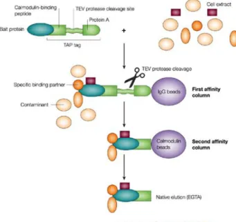
Biochemical methods [61, 86], such as tandem affinity purification followed by mass-spectrometric protein complex identification (TAP-MS) [198], provide a complementary approach to interaction mapping: these methods focus on identi-fying protein complexes. Although variations on the technique exist, the general principle is that a protein of interest is fused with a TAP tag, allowing the protein and its binding partners to be purified through affinity selection (Figure 1.4). Binding partners can then be identified through mass-spectrometry. The dis-advantage of these methods is that they are vulnerable to tagging disrupting

(23)

Figure 1.3: Illustration of a yeast two hybrid system. The bait (X), is fused to the DNA binding domain. A potential interactor or prey (Y) is fused to the activation domain (AD) The interaction of the bait and prey leads to recon-struction of a functional transcription factor, recruitment of RNA polymerase and transcription of the reporter gene. Figure reproduced from [24].

complex formation and to weakly associated components dissociating from the complex during the purification process [185].

Figure 1.4: Illustration of tandem affinity purification. The protein of interest (bait) is fused with a TAP tag, allowing it and its binding partners to be isolated through affinity purification. Figure reproduced from [91]

Data Quality

Assessing the quality of high throughput protein-protein interactions is a key step in using these data to make biological inferences. Estimating PPI data quality, however, is not necessarily trivial. A number of factors contribute to

(24)

the reliability of an experimental data set: the detection technique’s precision (the fraction of detected interactions that are true positives), its sensitivity (the fraction of true positives that the technique is able to detect) and any systematic biases in favour or against particular types of interaction.

One approach for determining false negative and false positive rates is to ex-amine the extent of overlap between different interaction data sets. Von Mering et al. found that, out of 80000 yeast protein interactions identified by vari-ous high throughput techniques, only 2400 were identified by more than one method [239]. While this low overlap could reflect high false positive rates, it is also possible the effect arises from low coverage or techniques exhibiting biases towards different types of interaction. Other authors have assessed overlap be-tween thesameaffinity purification technique performed by different groups and found only limited overlap between the detected interactions [60, 123, 171, 234]. Similarly, low overlap has also been reported when comparing yeast two hybrid data sets [188]. Again, however, these results may reflect low coverage rather than high false positive rate.

Other quality assessment approaches include comparing PPI data sets to benchmark sets of literature curated interactions, or evaluating the reliability of an interaction through the biological similarity of the interactors, in terms of, for example, correlation in expression patterns or shared biological function. The former approach is extremely sensitive to the choice of benchmark set and is affected by sociological biases in publication and curation processes [236]. Assessing interaction reliability through functional similarity, on the other hand, is dependent on the quality and coverage of functional annotation data, while the use of co-expression assumes interactors are necessarily co-expressed.

In order to circumvent these problems, Venkatesan et al. estimated the precision of yeast two hybrid screens by retesting a random subset of reported interactions using independent interaction assays [236]. This retesting suggested yeast two hybrid screens have a precision of around 80%, which was considerably higher than the precision (approximately 25%) for a literature curated set of interactions retested the same way. Interestingly, when data from TAP-MS screens is retested in a similar way, the performance is much poorer [253]. This difference between the techniques, however, is likely to reflect the difference in the type of interaction (i.e. protein complex co-membership rather than binary interaction) captured by the two techniques, rather than poor data quality from the TAP-MS screens. When the quality of TAP-MS data is assessed through other measures, such as shared biological function of interactors, TAP-MS and yeast two hybrid techniques yield comparable performance [253].

In terms of systematic bias, interaction sets are likely to favour evolutionarily conserved and high abundance proteins [239], although the bias towards highly expressed proteins is less pronounced in yeast two hybrid data. TAP-MS data has also been associated with under-representation of metabolic proteins and

(25)

over-representation of proteins involved in transcription and protein synthesis [255]. However, this probably reflects the differing involvement of protein complexes in these cellular functions, rather than bias in the technique itself. Interaction data is also biased against membrane protein complexes because lipid-anchored proteins are hydrophobic and thus more difficult to purify. Recently, affinity purification procedures optimised for membrane proteins have been developed to address this issue [11].

Finally, it is worth noting that the precision and sensitivity of detection techniques are only a partial measure of the usefulness of interaction data for biological inference: interactions captured byin vitro assays, even if genuine, do not necessarily have biological relevance. For example, it has been hypothesised that some interaction are evolutionary remnants of past function, but no longer play functional role in the cell [237]. Combining physical protein-protein inter-action data with other information capturing functional association (see below) has been suggested as a method for pruning out these ‘pseudointeractions.’

Data Integration

Combining data from multiple screens or sources can be an effective strategy for increasing coverage and reducing noise. Data integration is greatly aided by vari-ous public repositories (such as BioGRID [217], IntAct [109], MINT [136], HPRD [23], BIND [4] and DIP [205]) storing interaction data and various databases (for example STRING [101], I2D [23] and iRefIndex [194]) combining these reposito-ries into single datasets. As well as holding information from high-throughput screens, many of these repositories also collate results from smaller-scale studies of protein interaction.

Dataset Completeness

The mapping of the interactome, the complete set of protein-protein interactions, is still a work in progress. Even the concept of completion is not clearly defined: interactions are likely to be dependent on environmental conditions and cell type [21] and some interactions may, in practice, be undetectable [211]. It is therefore unclear whether the complete interaction should describe the full set of possible interactions [38] or whether maps should be cell type and condition specific.

Estimating how complete our current map of the interactome is difficult be-cause estimating the size of the full interactome is non-trivial. An empirical framework by Venkatesan et al., based on a literature-derived set of high quality true positives and performing repeated screens, gave an estimate of the size of the human interactome of 74000−200000 interactions [236]. Earlier estimates by Stumpf et al. suggested 650000 interactions for the human interactome and 25000–35000 for budding yeast [221]. BioGRID currently holds approximately

(26)

150000 unique physical interactions for human and 84000 for yeast and the num-ber of interactions appears to still be growing (Figure 1.5).

Figure 1.5: The number of unique physical protein-protein interactions in the BioGRID database in July of each year for budding yeast and human.

The incompleteness of the interactome introduces a concern that the network properties of the ‘true’ interactome may not be the same as those of the mapped sub-network.

Firstly, systematic bias in the detection method may mean that the proper-ties of the sampled sub-network do not reflect the properproper-ties of the underlying network. A trivial example would be, for example, under-representation of pro-teins not expressed in the nucleus in Y2H screens. More subtle effects have also been hypothesised. For example, Caldarelli et al. [26] studied network generation mechanisms where the probability of two nodes being connected is a function of an intrinsic property (‘importance’) of the nodes. The authors showed it is possi-ble to generate networks with power law degree distributions even in cases where the importance of the nodes is not power law distributed. For example, a net-work generation algorithm linking nodes if their combined importance exceeded a given threshold gave rise to networks with power law degree distributions even when the importance of the nodes followed an exponential distribution. This has implications for a number of detection techniques: Caldarelli’s results suggest that the power law degree distribution observed in protein interaction networks might not reflect the true properties of the network, but instead result from the probability of edge detection being dependent on properties of the proteins. In Y2H screens for example, being able to detect an interaction requires the correct

(27)

folding of the reconstructed transcription factor. It is not unrealistic to suggest this may in turn depend on intrinsic properties of the bait and prey proteins, such as size for example, thus leading to a potential distortion of the detected network’s degree distribution.

However, not all techniques will be subject to this type of bias. Thus, if the presence of heavy-tailed degree distributions in protein interaction networks were simply an artefact of the nature described by Caldarelli et al., we would expect different behaviour in networks derived with different techniques. A recent study reports that the properties of protein interaction networks are consistent across different detection techniques [99], suggesting these properties are not simply attributable to biases of individual techniques.

A second, more general concern is that even unbiased sampling may lead to distortion in the properties of the detected network. Analytical work by Stumpf et al. showed that, for networks with power law degree distributions, random node sampling does not result in the sampled sub-network having the same degree distribution as the original network [222]. Han et al. sampled edges from networks with random, exponential, power law, truncated normal degree distribution and found that the resulting sub-networks had similar degree distributions to Y2H-derived partial interactome maps [79]. These results again highlight the concern that incomplete PPI networks are not adequate proxies for the whole interactome and that the properties we observe in the incomplete network are an artefact of the sampling process. It is worth noting, however, that Han’s sampled sub-networks did not replicate all properties of the Y2H networks - the clustering coefficient of the sampled networks and real Y2H network, for example, were different [54].

Finally, incomplete coverage is not only a problem when looking at overall graph topology: it can also introduce bias into the network properties of indi-vidual nodes. For example, as discussed previously, not all protein interaction data originates from high-throughput screens: online repositories also integrate information from several smaller-scale studies. While this increases coverage, it also biases data towards well studied proteins: it is likely that proteins that are better studied will have more interactions in these datasets, potentially intro-ducing an artificial correlation between degree and features that are of interest to researchers, such as disease association or lethality.

To summarise, results derived from incomplete protein interaction networks may not apply to the full network. There have been some attempts to understand the nature of the bias introduced, but, without knowledge of the topology of the true network, this is a difficult task. The partiality of the coverage therefore needs to be taken into account when interpreting protein interaction networks. Fortunately, coverage of interaction networks is growing steadily. The biases introduced by network incompleteness are therefore likely to diminish with time.

(28)

Predicted Protein-Protein Interactions

Given the noise, bias and limited coverage of experimental interaction mapping techniques, computational approaches for predicting binding partners can offer a valuable complementary perspective. The term predicted protein interaction is used loosely in the literature: either to refer to predicted physical binding or to encompass methods indicative of more general functional association that may or may not involve direct physical contact between proteins [131]. This sec-tion will focus exclusively on predicted protein binding. More nebulous types of functional associations will be discussed in Section 1.4.4. In general terms, pre-diction approaches come in two flavours: biologically motivated methods, which seek to exploit biological insights to predict new interactors and statistical learn-ing methods, which seek to find features which correlate with protein interaction from various types of data, without explicitly requiring knowledge of biology.

There are various biological motivated approaches. The interaction of two proteins depends on their three dimensional features - many prediction methods therefore use protein structure to infer binding partners. For example, some approaches look for pairs of proteins exhibiting commonly interacting protein domains [114], while others seek to ‘inherit’ interactions from other organisms by identifying interacting pairs of homologs, using either sequence [150] or struc-ture [6, 7] based homology modelling. Recently, more direct methods have also been proposed: Wass et al. used protein docking algorithms, programs tradi-tionally used to predict the structure of complexes formed by known interactors, to detect new interaction partners [245]. While Wass et al. demonstrated this approach is feasible in principle, others have suggested the computational cost of a genome-wide docking-based approach would be prohibitively high [256]. Zhang et al. suggested a less computational intensive approach, based on mod-elling putative novel interactions on known interactions of structurally similar proteins [256]. Integrating other non-structural information to their prediction method and benchmarking against a set of high confidence interactors, Zhang et al. reported performance generally comparable to, and overall better than, high-throughput experimental methods.

Non-structure based prediction methods also exist. For example, some meth-ods exploit evolutionary relationships between proteins. Because physical inter-actions occur through the interinter-actions of specific residue interfaces on the pro-teins [232], interacting propro-teins are evolutionary linked: the deleterious effect of a mutation perturbing the interaction can be alleviated by a compensating mutation on the other protein. It is therefore possible to predict interaction based on correlated mutations [174] - this principle has lead to a number of methods predicting interactors based on similarity in the evolutionary history (phylogenetic trees) of proteins [37, 206].

Unlike the methods discussed so far, purely statistical approaches make mini-mal assumptions about the biological mechanisms governing protein interactions

(29)

- instead, given a set of ‘training examples’ (known interactors and (optionally) a set of known non-interactors) and some data about these examples, machine learning methods seek to identify data features that are predictive of the in-teractions. These methods have the advantage of potentially being capable of exploiting large volumes of heterogeneous data. For example, Pancaldi et al. built a predicted interaction network in fission yeast based on over 100 gene and protein features [168]. The disadvantage is that purely statistical methods are entirely dependent on the quality of the training examples.

Computational methods can also provide a useful tool for prioritising the testing of putative new interactions. However, it is important to note that these methods may be affected by biases in our current understanding of the interactome: computational methods are usually benchmarked against sets of high confidence interactions during development. Systematic biases in these benchmark sets may therefore affect how well computational methods appear to be performing.

Dynamic and Specific Protein Interaction Networks

Unlike the genome, the interactome is dynamic [21]. Protein expression varies between cell types and during development, meaning the interactome is depen-dent on both cell type and developmental context. Furthermore, many protein interactions are transient. Thus, even within a specific cellular and develop-mental context, the interactome is constantly changing. Recent work on PPI networks is seeking to recognise this: while dynamic or condition specific PPI data sets do not yet exist [94], a number of authors have attempted to combine gene expression and protein interaction data to create approximations of dynamic or condition specific networks. Examples of this approach will be discussed in detail in Chapter 5.

Recently, the effects of alternative splicing on protein interactions networks have also received more attention. This is particularly pertinent when working with human networks: current estimates suggest over 60% of human genes un-dergo alternative splicing [72,149,153]. Both Buljan et al. [25] and Weatheritt et al. [247] found that alternatively spliced regions in the human genome were en-riched in conserved protein-protein binding motifs, suggesting alternative splic-ing may give rise to tissue or cell type specific interactions. Ellis et al. [47] tested this idea experimentally by examining the effect of including or excluding brain specific exons in a number of mouse genes - they found that approximately a third of the alternative splicing events lead to changes in the interactions of the gene products. Davis et al. [40] used a bioinformatic approach to examine the effect of alternative splicing on protein interaction domains, finding evidence for altered interactions in almost 20% of genes. Interestingly, both Buljan et al. and Ellis et al. report that proteins affected by tissue-specific splicing have higher degree and centrality in PPI networks, suggesting alternative splicing is likely to

(30)

play a significant role in altering network topology. These results suggest that alternative splicing may fine-tune PPI networks in a tissue-specific manner.

1.4.2 Co-Expression Networks

In co-expression networks, edges between genes capture high levels of similarity in expression patterns. The rationale behind the study of these networks is that genes with similar function tend to have similar patterns of expression [46] - co-expression networks therefore provide a perspective on functional associations between genes. The advantage of working with co-expression networks is that many of the concerns raised in relation to PPI network bias and incompleteness are not relevant. Furthermore, condition and cell type specific networks are readily available. On the other hand, the functional significance of co-expression is less clear than that of direct binding and co-expression network generation is associated with its own set of statistical problems.

Network Generation

Co-expression networks are conceptually straightforward, but the details of net-work generation can vary considerably between studies. The most common ap-proach is to use some measure of similarity in expression as a basis for network generation. Various metrics have been proposed. The simplest method is the use of a correlation (either Pearson, see, for example [44] or Spearman see, for example [9]) metric. More sophisticated approaches have been proposed, al-though it remains unclear whether these offer real benefits. For example mutual information based measures have been used to capture non-linear correlations in gene expression [39]. However, estimating mutual information from expres-sion data can be computational intensive and it remains unclear whether mutual information captures meaningful biological relationships [216]. Networks are nor-mally generated by considering genes with a high correlation magnitude and/or significance value. Here, again, specifics of approaches differ on a number of methodological points: whether absolute values of correlation magnitude are used when thresholding; whether only magnitude or magnitude and significance of the correlation are considered; whether significance values are corrected for multiple testing; whether the resulting network is weighted or unweighted.

A drawback of using correlation-based methods is that they cannot distin-guish between direct and indirect dependencies: two genes may be co-expressed because one regulates the other, or because they are both co-regulated by the same transcription factor [148]. Recently, probabilistic graphical models have been suggested as a potential solution to this issue. Probabilistic graphical mod-els use a network representation to encode a probability distribution: nodes rep-resent variables of interest and edges reprep-resent conditional dependence. Thus, probabilistic graphical model approaches seek to find the pattern of conditional

(31)

dependencies that best explain the gene expression data. These methods include graphical Gaussian models [177, 208] and bayesian network [31, 156] approaches. Allen et al. [5] performed a comprehensive comparison of different network generation approaches, using both simulated data and real expression data from E. coli. Correlation, mutual information and partial correlation based methods all performed comparably in constructing global network topology, with partial correlation based methods being particularly good at identifying few connections with high specificity. Bayesian networks were found to be hindered by their poor scalability to large datasets.

Co-Expression Data

Until recently, co-expression networks were typically generated from microarray data. Microarrays are a hybridization based technology: sets of one-stranded DNA probes are incubated with fluorescence labelled target sequences. The hybridization of complementary sequences allows inferring the expression levels of sequences corresponding to particular probes. Recently however, progress in transcriptome sequencing (RNA-seq) technologies has allowed the construction of co-expression networks from RNA-seq data. RNA-seq data has the advantage of not having to pre-define the sequences to be measured, not being subject to noise from cross-hybridization and having a greater dynamic range than microar-rays [243]. RNA-seq datasets also allow study of novel [200] and alternatively spliced [197] transcripts. On the other hand, there are also concerns relating to RNA-seq data quality: the technique struggles with identification of rare transcripts (as these get obscured by the wide dynamic range) and exhibits a bias towards longer genes (because longer sequences generate more reads) which has not yet been fully addressed by existing normalization methods [225]. It is also worth noting that networks generated from microarray and RNA-seq data may not capture the same functional relationships. In a comparative study of Arabidopsis co-expression networks, overlap between RNA-seq and microarray network was low, with microarray networks having higher similarity to known biological networks [68].

Co-Expression Network Analysis

Topological analysis of co-expression networks has focused, to a large extent, on identifying highly connected nodes and detecting network modules [56]. For example, comparison of network modules and hubs in normal and disease co-expression networks is used to suggest candidate genes for disease association [238]. Guilt-by-association type approaches have also been applied in the context of co-expression results, for example in identifying new players in B-cell signal transduction [16] and plant cell wall synthesis [179].

The analysis and interpretation of the global topological properties of co-expression networks can be confounded by the way they are generated. For

(32)

example, correlation is transitive: if A correlates with B and B correlates with C, A and C are also likely to be correlated. The high clustering coefficient of co-expression networks therefore simply reflects this property and cannot be considered indicative of the functional properties of the cell [218]. This also has implications for null model selection: configuration models (networks with the same degree distribution but reshuffled edges) are not necessarily appropriate null models for co-expression networks. Null models generated by computing new networks from permuted versions of the original expression data may therefore be more appropriate under some circumstances.

1.4.3 Genetic Interaction Networks

A genetic interaction between two genes refers to the emergence of an unexpected phenotype when variation in the two genes co-occurs. The effect can be negative, for example loss of function in one gene being lethal only when function is also lost in some specific other gene (synthetic lethality), as well as positive, for example when the deleterious phenotype of one mutation is rescued by mutation in another gene. These types of interactions are of great interest, because they are thought to play a role in the complexity of biological organisms - for example, in the genetics of complex disease [8].

Genetic interaction networks have been extensively mapped in a number of singled celled organisms, particularly in budding yeast (Saccharomyces cere-visiae) [36, 228]. The topology of these networks appears functionally informa-tive in a way reminiscent of PPI networks: similar biological processes cluster together and node degree correlates with functional importance of the node. Genetic interaction networks have also been suggested as tools for identifying potential drug targets [36].

1.4.4 Other Functional Association Networks

Protein-protein, co-expression and genetic interaction networks are perhaps the most well studied of gene and protein networks. However, there are a number of other methods of inferring functional association between genes. This section will briefly outline these other forms of interaction.

Genomic Context

These methods seek to use genomic information to infer functional associations between genes. One approach is to look at whether gene pairs appear together on multiple genomes: if two gene products need to interact to function correctly, they are more likely to be co-inherited, as loss of one protein would impair the function of the other [176]. We can thus use the correlated absence or pres-ence of gene pairs across multiple genomes (‘phylogenetic profile’) to infer as-sociation. Because of greater availability of sequences genomes in prokaryotes