A decision procedure for satisfiability in separation logic with inductive predicates

A Decision Procedure for Satisfiability in

Separation Logic with Inductive Predicates

James Brotherston

Carsten Fuhs

Juan A. Navarro P´erez

{j.brotherston,c.fuhs,juan.navarro}@ucl.ac.uk

Nikos Gorogiannis

Abstract

We show that the satisfiability problem for the “symbolic heap” fragment of separation logic with general inductively defined pred-icates — which includes most fragments employed in program ver-ification — isdecidable. Our decision procedure is based on the computation of a certain fixed point from the definition of an in-ductive predicate, called its “base”, that exactly characterises its satisfiability.

A complexity analysis of our decision procedure shows that it runs, in the worst case, in exponential time. In fact, we show that the satisfiability problem for our inductive predicates is EXPTIME-complete, and becomes NP-complete when the maximum arity over all predicates is bounded by a constant.

Finally, we provide an implementation of our decision proce-dure, and analyse its performance both on a synthetically gener-ated set of test formulas, and on a second test set harvested from the separation logic literature. For the large majority of these test cases, our tool reports times in the low milliseconds.

Categories and Subject Descriptors F.3.1 [Logics and Mean-ings of Programs]: Specifying and Verifying and Reasoning about Programs—Mechanical verification, assertions; F.2.2 [Analysis of Algorithms and Problem Complexity]: Nonnumerical Algorithms and Problems—Complexity of proof procedures

General Terms Algorithms, Theory, Verification

Keywords separation logic, inductive predicates, satisfiability, de-cision procedure

1.

Introduction

Separation logic[26] is an established and fairly popular formal-ism for verifying imperative, heap-manipulating programs. At the

∗_{Research supported by an EPSRC Career Acceleration Fellowship.} †_{Research supported by EPSRC grants EP/K040863/1 and EP/H008373/2.} ‡_{Research supported by EPSRC grants EP/K040863/1 and EP/K032542/1.}

Permission to make digital or hard copies of part or all of this work for personal or classroom use is granted without fee provided that copies are not made or distributed for profit or commercial advantage and that copies bear this notice and the full citation on the first page. Copyrights for third-party components of this work must be honored. For all other uses, contact the owner/author(s).

CSL-LICS 2014, July 14–18, 2014, Vienna, Austria. Copyright is held by the owner/author(s).

ACM 978-1-4503-2886-9/14/07. http://dx.doi.org/10.1145/2603088.2603091

time of writing, there are a number of automatic program verifi-cation tools based on separation logic, such as SLAYER[5] and ABDUCTOR[12], capable of establishing memory safety properties of code bases extending into millions of lines [28]. These verifica-tion tools are highly dependent on the use ofinductively defined predicatesto describe the shape of data structures held in mem-ory, such as linked lists or trees. Currently, such predicates must be hard-coded into these verification tools, which limits the range of data structures that they can handle automatically. Thus, the next step in automation is to handlegeneralinductive predicates, which might be provided to the analysis by the user, or even inferred auto-matically [10]. When one considers arbitrary inductive predicates, however, it becomes much more difficult to determine whether a given formula issatisfiableor not. This may lead to performance degradation when time is spent on the analysis of inconsistent sce-narios.

In this paper we address the latter problem by showing that the satisfiability problem for the most commonly consideredsymbolic heapfragment of separation logic, extended with general inductive predicates, is in factdecidable. Our decision procedure rests upon the observation that the satisfiability of each inductive predicate can be precisely characterised by an approximation of its set of models, an object which we refer to as thebaseof the predicate. Roughly speaking, the base of a predicate records, for each distinct way of constructing a satisfying model, the subset of arguments of the predicate that are required to be allocated and distinct in memory, as well as the equalities and disequalities that must hold between these arguments. Since there are clearly only finitely many possible such subsets and equality/disequality relations between predicate arguments, the base can be straightforwardly computed in finite time. Having computed the base of all required predicates, deciding the satisfiability of arbitrary formulas in the fragment then becomes a straightforward matter.

A complexity analysis of our decision procedure shows that, in the worst case, it runs in exponential time (in the size of the underlying set of inductive definitions). Essentially, this is because our inductive definition schema allows us to construct predicates that admit an exponential number of elements in their base. Indeed, we show that the satisfiability problem for our inductive predicates isEXPTIME-complete. Additionally, if the maximum arity of all inductive predicates is bounded, then the satisfiability problem becomesNP-complete.

We also provide an implementation of our decision procedure, which is available online [1], and evaluate its performance over three test sets: (a) a collection of example formulas drawn from the literature on separation logic verification; (b) a large set of in-ductive predicates automatically generated by the CABER predi-cate inference tool [10]; and (c) a set of synthetically generated examples, varying in parameters such as the number of arguments

or recursive calls. Although exponential time performance can be produced by a suitable choice of parameters, we find that for the vast majority of examples, the algorithm terminates in a matter of milliseconds. Consequently, we believe our decision procedure is highly suitable for use as a black-box satisfiability checker in auto-mated separation logic verification. We propose a number of direct applications of such a satisfiability checker at the end of this paper (in Section 7).

The problem of satisfiability for separation logic with induc-tive definitions was also recently considered by Iosif et al. [20]. Their paper establishes decidability results for both satisfiability

andentailment problems via an embedding into monadic second order logic, but for technical reasons their results are restricted to a fragment of the logic from which many natural data structure def-initions are excluded; for example, inductive predicates may not define structures with dangling data pointers (cf. Section 6.1). In contrast, the fragment of separation logic for which we decide sat-isfiability includes a much larger class of inductive predicates, but we do not consider the entailment problem for this fragment, which isundecidable[2]. We also provide complexity results on the sat-isfiability problem for our fragment, and an implementation of our decision procedure.

The remainder of this paper is structured as follows. We intro-duce our fragment of separation logic with inductive definitions in Section 2, and then present our decision procedure and the proof of its correctness in Section 3. Section 4 contains our complexity analysis of our algorithm and of the satisfiability problem itself. Section 5 describes the implementation of our decision procedure and its evaluation. Section 6 surveys related work in the area, and Section 7 concludes.

2.

Inductive definitions in separation logic

Here we present our fragment of inductive definitions in separation logic, following the approach in [9].

2.1 Syntax

First, some preliminaries. Atermis either avariabledrawn from the infinite setVar, or the constant symbolnil. We writeTermfor the set of all terms. We also assume a fixed finite setP1, . . . , Pn ofpredicate symbols, each with an associated arity. We often write vector notation to abbreviate tuples; e.g. we typically writexrather than(x1, . . . , xm). We writeπi(−)for thei-th projection function on tuples, and sometimes abuse notation slightly by writingx∈x

to mean thatxoccurs in the tuplex. Finally, we writePow(X)for the powerset of a setX.

Definition 2.1. Spatial formulasFandpure formulasGare given by the following grammar:

F::=emp|t7→t|Pit|F∗F

G::=t=t|t6=t

wheretranges over terms,Piover the predicate symbols andtover tuples of terms (matching the arity ofPiinPit). We writePureSet for the set of allfinite setsof pure formulas.

Asymbolic heapis given byΠ :F, whereFis a spatial formula andΠ ∈ PureSet(note thatΠshould be read intuitively as the conjunction of its elements). Whenever one ofΠ, F is empty, we will omit the colon.

We write the substitution notationF[t/x]for the result of simul-taneously replacing all occurrences of the variablexby the termt

in the formulaF. Substitution extends to sets of formulas in the obvious way.

Definition 2.2. An inductive rule set is a finite set ofinductive rules, each of the formΠ :F ⇒Pix, whereΠ :Fis a symbolic

heap,Piis a predicate symbol of arityai, andxis a tuple ofai distinct variables.

Variables in the body,Π :F, but not the head,Pi(x), of a rule are implicitly existentially quantified, while multiple bodies of the same head are interpreted as a disjunction. The formal semantics is given in the next section.

Our strict formatting of the heads of inductive rules, with vari-able repetitions and occurrences of nil disallowed, is for tech-nical convenience. It does not restrict expressivity since we can achieve the same effect by placing equalities in the bodies of in-ductive rules. For example, a rule of the form ⇒ P(x, x,nil)

is not allowed by our schema, but the equivalent inductive rule

x=y, z=nil⇒P(x, y, z)is allowed. 2.2 Semantics

We use a typical RAM model employing heaps of records. An infinite setValofvalues is assumed, of which an infinite subset Loc⊂Valarelocations, i.e., the addresses of heap cells. We also assume a “nullary” valuenil∈Val\Locwhich is not the address of any heap cell. Astackis a functions:Var→Val; we extend stacks to terms by settings(nil) =def nil, and extend stacks pointwise to act on tuples of terms. We writes[x7→v]for the stack defined as

sexcept that(s[x7→v])(x) =v.

A heap is a partial functionh:Loc*fin(Val List) mapping finitely many locations to (arbitrary-length) tuples of values; we define

dom(h) =def{`∈Loc|h(`)is defined}

and e to be the empty heap that is undefined everywhere. We write◦to denotecompositionof heaps: ifh1 and h2 are heaps,

thenh1◦h2 is the union of (partial functions)h1 andh2 when dom(h1)∩dom(h2) = ∅, and undefined otherwise. We write

h[`7→v]for the heap defined ashexcept that(h[`7→v])(`) =v, and just[`7→v]as a shorthand fore[`7→v]. We writeHeapfor the set of all heaps.

Given an inductive rule set Φ, the relation s, h |=Φ F for

satisfaction of a pure or spatial formulaFby the stacksand heaph

is defined as follows: s, h|=Φt1=t2 ⇔ s(t1) =s(t2) s, h|=Φt16=t2 ⇔ s(t1)6=s(t2) s, h|=Φemp ⇔ h=e s, h|=Φt7→t ⇔ dom(h) ={s(t)}andh(s(t)) =s(t) s, h|=ΦPit ⇔ (s(t), h)∈_JPi_KΦ s, h|=ΦF1∗F2 ⇔ h=h1◦h2ands, h1|=ΦF1 ands, h2 |=ΦF2

where the semanticsJPiK

Φ

of the inductive predicate Pi under

Φis defined below. IfΠ : F is a symbolic heap then we write

s, h|=Φ Π : F to mean thats, h |=Φ F ands, h|=Φ Gfor all

G∈Π; equivalently, we say that(s, h)is amodelofΠ :F(w.r.t.

Φ). A symbolic heapΠ :Fissatisfiable(w.r.t.Φ) if it has at least one model.

We remark that satisfaction of pure formulas does not depend on the heap nor on the inductive rules: we writes |= Π, where

Π∈PureSet, to mean thats, h|=ΦΠfor any heaphand inductive

definition setΦ.

The following definition gives the standard semantics of the inductive predicate symbolsPaccording to a fixed inductive rule setΦ, i.e., as the least fixed point of ann-ary monotone operator constructed fromΦ:

Definition 2.3. First, for each predicatePi∈Pwith arityaisay, we defineτi = Pow(Valai×Heap). Furthermore, we partition

the rule setΦintoΦ1, . . . ,Φn, whereΦiis the set of all inductive rules inΦof the formΠ :F ⇒Pix.

We let eachΦibe indexed byj(i.e.,Φi,jis thej-th rule defining

Pi), and for each inductive ruleΦi,jof the formΠ :F ⇒Pix, we define the operatorϕi,j:τ1×. . .×τn→τiby:

ϕi,j(Y) =def{(s(x), h)|s, h|=XΠ :F}

whereY∈τ1×. . .×τnand|=Yis the satisfaction relation defined above, except that_JPiK

Y ₌

def πi(Y). We then finally define the tuple_JP_KΦ_∈τ 1×. . .×τnby: JPK Φ =defµY.(Sjϕ1,j(Y), . . . , S jϕn,j(Y)) We write_JPiK Φ_{as an abbreviation forπ} i(JPK Φ_).

As in [9], Definition 2.3 interprets the inductive rulesΦi as

exhaustive, disjunctive clausesof the definition of the predicatePi.

3.

A decision procedure for satisfiability of

inductive predicates

In this section, we present our decision procedure for satisfiability in the symbolic heap fragment of separation logic with inductive predicates, given in Section 2.

Our first definition is used to normalise terms in pure formulas with respect to a given set of variables. This is then used in our second definition, which provides a satisfiability-preserving means of restricting the variables which occur in a set of pure formulas. Definition 3.1. LetΠ ∈ PureSetand letxbe a tuple of distinct variables. The equalities inΠ determine an equivalence relation among terms. We say that an equivalence class isobservable (from

x with respect to Π), if the class contains some term in x∪ {nil}. A term is observable just in case it belongs to an observable equivalence class.

For each equivalence class, we choose a term from the class, called its canonical representative. For observable classes, we choosenilto be the representative ifnilis in the class, otherwise we choose a variable fromx. For non-observable classes, the choice is arbitary. Thenormal formof a termt, denotedhtiΠ,x, is defined to betitself whent∈x∪ {nil}, or the canonical representative of its equivalence class otherwise.

Definition 3.2. LetΠ ∈ PureSetand letxbe a tuple of distinct variables. We denote by Π x the formula obtained after: (i) removing all pure formulas,t1 = t2 ort1 6= t2, where at least

one oft1 ort2is not observable; and (ii) replacing all remaining

termstby their normal formshtiΠ,x.

Note that Definition 3.2 ensures every term occurring inΠxis eithernil, or a variable fromx. The satisfiability-preserving nature of this variable restriction is formalised by the following pair of lemmas.

Lemma 3.3. LetΠbe a finite set of pure formulas. Ifs|= Πand

s(x) =s0(x)thens0|= Πx.

Proof. Sinces|= Π, we know thatsmust assign the same value to all variables sharing the same equivalence class. Thuss|= Πx, since both dropping formulas fromΠand replacing terms by their normal forms preserve its satisfiability.

Now,Πxis restricted to contain only variables fromxand, sincesands0agree on those variables,s0|= Πx.

Lemma 3.4. LetΠbe a finite set of pure formulas. If Πis satisfi-able ands|= Πxthen there exists a stacks0withs0(x) =s(x)

such thats0|= Π.

Furthermore, given any finite setW ⊆Loc, we can chooses0

such thats0(y)∈/Wfor all non-observable variablesy.

definebaseΦ_P

:

Y:= (λt1.∅, . . . , λtn.∅) repeat untilYreaches a fixed point:

pick a ruleΦi,j ∈Φwith headPix for eachPj`(x`)in the body ofΦi,j:

pick a base pair(V`,Π`)∈Yj`(x`)

takey1, . . . , ykfrom ally`7→u`in the body ofΦi,j takeΠ0the pure part in the body ofΦi,j

V :=V1∪ · · · ∪Vm∪ {y1, . . . , yk} Π :=N V ∪Π0∪Π1∪ · · · ∪Πm ifΠis satisfiable: add alloced(V,x,Π)[t/x],(Πx)[t/x] toYi(t) returnY

Figure 1. Pseudocode for the computation ofbaseΦPin Defn. 3.5.

Proof.Let Y1, . . . , Yn be the equivalence classes of all vari-ables occurring in, and determined by,Π. Choose distinct values

`1, . . . , `ninLocsuch that each`i ∈/ s(x∪ {nil})∪W. This is possible because the number of locations inLocis infinite, while the number of forbidden locations is finite. We then define

s0(x) =

(

s(hxiΠ,x) ifxis observable

`i otherwise, wherex∈Yi. By constructionsands0 agree on variables fromx, i.e. directly observable ones, ands0(y) ∈/ W whenyis not observable. It is easy to check now thats0satisfies all pure formulas inΠ.

• For everyt1=t2∈Π: By definition,t1andt2are in the same

equivalence class. Thus ift1is observable then so, necessarily,

is t2, and furthermore the formulaht1iΠ,x = ht2iΠ,x is in

Π x. Therefore, by assumption, s |= ht1iΠ,x = ht2iΠ,x, and sinces0(ti) =s(htiiΠ,x), we haves0|=t1=t2.

Otherwise, ift1is not observable, then neither ist2; but, since

they share an equivalence class, we haves0(t1) =`i=s0(t2)

for someiby construction, and sos0|=t1=t2as required.

• For every t1 6= t2 ∈ Π: If botht1 and t2 are observable,

then ht1iΠ,x 6= ht2iΠ,x is in Π x, so s |= ht1iΠ,x 6= ht2iΠ,xby assumption. Since s0(ti) = s(htiiΠ,x), it follows thats0|=t16=t2.

If one of the terms, say t1, is observable but the other, t2,

is not, then s0(t2) was explicitly chosen to be different to

s(ht1iΠ,x) =s0(t1), and sos0|=t16=t2.

If neithert1nort2is observable, then they must be in different

equivalence classes, otherwiseΠwould be unsatisfiable, con-trary to assumption. Thus, by construction,s0|=t16=t2.

We now present our main definition, which explains how to ex-tract from a fixed inductive rule setΦall the information needed to decide the satisfiability of any symbolic heap overΦ. The pseu-docode in Figure 1 provides an informal aid to navigate the steps of the computation.

Definition 3.5(Base pair computation). First, for each predicate symbolPiwith associated arityai, where1≤i≤n, we define

σi=defTermai→Pow(MPow(Var)×PureSet) whereMPow(Var)denotes the set of all multisets of variables. For any finiteV ∈MPow(Var)we defineN

V ∈PureSetto be the set of pure formulas comprising:

•all formulas of the formx6=x0such thatxandx0are different elements ofV (note this means that ifV contains duplicates thenN

V is unsatisfiable);

•the formulax6=nilfor every elementxofV.

For any finite multiset V of variables, any tuple of variables

x, and anyΠ ∈ PureSet, let alloced(V,x,Π)denote the mul-tiset containing the term hyiΠ,x for each y ∈ V observable from xwith respect to Π. Note that if Π∪N

V is satisfiable, thenalloced(V,x,Π)contains only variables (nonil) and no du-plicates. In this way we represent, using only variables fromx, the observable locations allocated viaV.

The inductive rule setΦ is partitioned intoΦ1, . . . ,Φn with eachΦifurther indexed byjas in Definition 2.3. Without loss of generality, we consider eachΦi,j∈Φto be written in the form

Π0:y17→u1∗. . .∗yk7→uk∗

Pj1(x1)∗. . .∗Pjm(xm)⇒Pix, (IndRule)

whereΠ0 ∈ PureSet. We use the inductive rule Φi,j to define an operator Ψi,j: σ1 ×. . . ×σn → σi as follows. If Y =

(Y1, . . . , Yn)where each Yi ∈ σi, andtis a tuple ofaiterms, thenΨi,j(Y) :σisendstto the set of pairs (we shall call these pairs alsobase pairs)

alloced(V,x,Π)[t/x],(Πx)[t/x] that satisfy the following:

V =V1∪ · · · ∪Vm∪ {y1, . . . , yk}, Π =N

V ∪Π0∪Π1∪ · · · ∪Πmis satisfiable, and∀1≤`≤m.(V`,Π`)∈Yj<sub>`</sub>(x`).

Note that the substitution[t/x]in the above is defined pointwise over tuples; this is well defined sincexis a tuple ofdistinct vari-ables, as per Definition 2.2. Note also that whilealloced(V,x,Π)

might be viewed as a set (i.e., without repetitions), it is important to understandalloced(V,x,Π)[t/x]as a multiset since the substi-tution may map different variables to the same term.

We then definebaseΦ_P∈σ

1×. . .×σnas follows: baseΦP=defµY.(SjΨ1,j(Y), . . . ,SjΨn,j(Y)) where, by pointwise extension of the union to act on functions, we writeS

jΨi,j(Y)to denote the function mapping a tuple of terms

tto the setS

jΨi,j(Y)(t). We also writebase

Φ

Pito abbreviate

πi(baseΦP).

Example 3.6. Consider the following setΦof inductive rules:

Φ1,1: x=nil⇒P(x)

Φ1,2: x6=nil:Q(x, x)⇒P(x) Φ2,1: y=nil, x6=nil:x7→(d, c)∗P(d)⇒Q(x, y) Φ2,2: y6=nil:y7→(d, c)∗Q(x, c)⇒Q(x, y).

These rules are an intermediate product of the analysis done by the tool CABER[10] on code that traverses a list of lists, and are found to be ultimately unsatisfiable by our algorithm, triggering back-tracking in CABER. In accordance with Definition 3.5, we define:

σ1=Term→Pow(MPow(Var)×PureSet)

σ2=Term×Term→Pow(MPow(Var)×PureSet).

That is,σ1andσ2are function spaces mapping suitably many terms

to sets of base pairs forP andQ, respectively. We can compute baseΦ_{(P, Q)}

by iteratively computing the sequence of its fixed point approximants((Y1i, Y

i

2)∈σ1×σ2)i≥0in the standard way.

That is, we begin with an empty base for both predicates, namely

Y0 = (λx.∅, λx, y. ∅), and iteratively apply the operatorsΨi,j given by Definition 3.5.

First iteration:The inductive ruleΦ1,1forP(x)can be applied

toY0_{, yieldingV =∅andΠ ={x=nil}. The setΠis satisfiable}

and, therefore, Ψ1,1(Y10, Y 0 2) =λx. (∅,{x=nil}) .

SinceY0 does not contain any base pairs, the remaining rules cannot be applied to it, and soY1= (Y11, Y21)where

Y11=λx.

(∅,{x=nil})

Y21=λx, y.∅.

Second iteration: The inductive ruleΦ1,1 generates the same

base pair as before, whileΦ1,2andΦ2,2are still not applicable to

Y1

. However, the ruleΦ2,1definingQ(x, y)can be now applied,

taking(∅,{x = nil}) from the current baseY11 ofP(x). After

restricting and normalising to the set of observable variables, this produces the new base pair({x},{y=nil, x6=nil}). Thus, at the end of the iteration,Y2_{= (Y}2

1, Y22)where Y12=λx. (∅,{x=nil}) Y22=λx, y. ({x},{y=nil, x6=nil}) .

Third iteration: The rule Φ1,2 is now applicable to Y2,

in-stantiating the current pair forQ(x, x), but yields an unsatisfi-ableΠ. Similarly, the ruleΦ2,2can be applied, taking the base pair ({x},{c= nil, x 6=nil})fromY22instantiated toQ(x, c). After

a suitable variable restriction and normalisation, this produces the following new base pair forQ(x, y):

({x, y},{x6=y, y6=nil, x6=nil}) ThusY3= (Y13, Y 3 2)where Y13=λx. (∅,{x=nil}) Y23=λx, y. _{({x},{y=nil, x6=nil}),} ({x, y},{x6=y, y6=nil, x6=nil}) .

On the fourth iteration no new base pairs are produced — both

Φ1,2 andΦ2,2can be applied to the newly created base pair from

the latest iteration, but the former yields an unsatisfiableΠand the latter reproduces the same base pair — so we have reached a fixed point, andbaseΦ(P, Q) = (Y13, Y23).

The next two lemmas formalise the fact thatbaseΦP(x) pre-cisely characterises the satisfiability ofP(x).

Lemma 3.7 (Soundness). Given a base pair (V,Π) ∈

(baseΦ_P

i)(t), a stack s such that s |= Π, and a finite set

W⊆Loc\s(V), there exists a heaphsuch thats, h|=ΦPitand

dom(h)∩W =∅.

Proof.We proceed by fixed point induction on the definition of baseΦP. That is, we assume the lemma holds for a tuple of func-tionsY = (Y1, . . . , Yn) ∈ σ1 × · · · ×σn, and we must show

it also holds for(S

jΨ1,j(Y), . . . , S

jΨn,j(Y)). Thus, assume

(V,Π)∈Ψi,j(Y)(t)withs|= Πands(V)∩W =∅. We require to find anhwiths, h|=Pitanddom(h)∩W =∅.

By assumption, there is a ruleΦi,jof the form (IndRule) with

(V,Π) ∈ Ψi,j(Y)(t). ThereforeV = alloced(V0,x,Π0)[t/x] andΠ = (Π0x)[t/x], where the following hold:

V0=V1∪ · · · ∪Vm∪ {y1, . . . , yk}, Π0=N

V0∪Π0∪Π1∪ · · · ∪Πmis satisfiable, ∀1≤`≤m.(V`,Π`)∈Yj`(x`).

By the lemma assumption and usual substitution facts, we have that

s[x7→s(t)]|= Π0xand

s[x7→s(t)](alloced(V0,x,Π0))∩W =∅.

SinceΠ0is satisfiable, we can apply Lemma 3.4 to obtains0with

s0(x) = s[x 7→ s(t)](x) = s(t) and s0 |= Π0. Furthermore, the lemma tells us that for any non-observabley ∈ V0, we have

y /∈W. Otherwise, ify∈V0is observable fromxw.r.t.Π0, there is anx ∈ x such that yand xare in the sameΠ0-equivalence class. It follows that s0(y) =s0(x) =s[x7→s(t)](x) and, as

x∈alloced(V0,x,Π0) but s[x 7→ s(t)](alloced(V0,x,Π0))∩

W =∅, it must be the case thats0(y)∈/W. Thus, for ally∈V0

we haves0(y)∈/W, that iss0(V0)∩W =∅.

We now show that there are heapsh1, . . . , hmsuch that, for all

1≤`≤m, we have boths0, h`|=ΦPj`x`anddom(h`)∩W`=

∅, whereW`is defined as follows:

W`=defW∪s 0 ({y1, . . . , yk})∪ [ p<` dom(hp)∪ [ `<q≤m s0(Vq).

To do this, we inductively assume that we have constructed the chain of heaps(hp)1≤p<`, and show how to constructh`. Inductive construction ofh`from(hp)1≤p<`:We claim and prove thats0(V`)∩W`=∅. We have shown thats0(V0)∩W =∅; since

V`⊆V0, it follows thats0(V`)∩W = ∅. Next, letp < `and note that the induction hypothesis implies dom(hp)∩Wp=∅, which in turn implies dom(hp)∩s0(V`) =∅ by definition of

Wp. Thuss0(V`)∩Sp<`dom(hp) = ∅. Next, let q > `and notice that s0(V`) ∩s0(Vq) = ∅ because s0 |= NV0, which guarantees thats0 is injective onV0 ⊇ V`, Vq. It therefore fol-lows thats0(V`)∩S_`<q≤ms

0

(Vq) =∅. Also, for a similar reason,

s0(V`)∩s0({y1, . . . , yk}) =∅.

Now(V`,Π`)∈Yj`(x`), wheres 0_|

= Π`ands0(V`)∩W`=∅, so by the main induction hypothesis (of the fixed point induction for the present lemma) there is a heaph`such thats0, h` |=Φ Pj`x`

anddom(h`)∩W`=∅. This completes the construction ofh`. We continue with the main proof. Note that h1 ◦. . .◦hm is defined because dom(h`)∩W` = ∅ for all 1 ≤ ` ≤ m implies thatdom(h1), . . . ,dom(hm) are all disjoint from each other. Now we define a heaph0whose domain iss0({y1, . . . , yk})

as follows:h0(s0(yi)) =def s0(ui)for each1≤i≤k. Note that

h0◦(h1◦. . .◦hm)is defined becauses0|=NV0ensures thats0 is injective on{y1, . . . , yk} ⊆V0anddom(h`)∩W`=∅ensures thatdom(h`)∩dom(h0) =∅for each1≤`≤m. Thus, defining

h=defh0◦h1◦. . .◦hm, we obtain:

s0, h|=ΦΠ0 :y17→u1∗. . .∗yk7→uk∗Pj1x1∗. . .∗Pjmxm which implies thats0, h|=ΦPix(by applying the operatorϕi,j). Thus, sinces0(x) =s(t), we obtains, h|=ΦPit.

We havedom(h)∩W =∅as required because

dom(h`)∩W ⊆dom(h`)∩W`=∅,

for each1≤`≤m, anddom(h0) =s0({y1, . . . , yk})⊆s0(V0)

whiles0(V0)∩W =∅.

Lemma 3.8(Completeness). Ifs, h|=ΦPit, there is a base pair

(V,Π)∈(baseΦPi)(t)such thats(V)⊆dom(h)ands|= Π.

Proof. We have that(s(t), h) ∈ _JPi_KΦ, and apply fixed point induction on the definition of JPK

Φ

. That is, we assume the lemma holds for X = (X1, . . . , Xn) ∈ τ1 ×. . .×τn and must show that it holds for(S

jϕ1,j(X), . . . , S

jϕn,j(X)). Thus, assuming that (s(t), h) ∈ ϕi,j(X), we must then find a pair

(V,Π)∈(baseΦPi)(t)withs(V)⊆dom(h)ands|= Π.

By assumption, there is an inductive rule Φi,j of the form (IndRule) such that (s(t), h) ∈ ϕi,j(X). By construction this means thats(t) =s0(x)for some stacks0, and we have

s0, h|=XΠ0:y17→u1∗. . .∗yk7→uk∗Pj1x1∗. . . Pjmxm Thuss0 |= Π0 and h = h1◦. . .◦hk◦h01 ◦. . .◦h0m, where

s0, h` |=Φ y` 7→ u`for all1 ≤`≤ k, and(s0(x`), h0`) ∈ Xj`

for all1 ≤ ` ≤ m. Then, by the induction hypothesis, for all

1≤`≤mthere are pairs(V`,Π`)∈(baseΦPj`)(x`), such that

s0(V`)⊆dom(h0`)ands 0_| = Π`. Now we define V =def [ 1≤`≤m V` ∪ {y1, . . . , yk}.

Asdom(h1), . . . ,dom(hk),dom(h01), . . . ,dom(h0m)are all dis-joint, wheredom(h`) = {s0(y`)} for each 1 ≤ ` ≤ k and

dom(h0`) ⊇ s

0

(V`)for each1 ≤ ` ≤ m, we haves0 |= NV (i.e.,hwould be undefined ifs0were not injective onV). Putting everything together, we have

s0|= Π0∪NV ∪Π1∪ · · · ∪Πmands0(V)⊆dom(h). ThusΠ = Π0∪NV ∪Π1∪ · · · ∪Πmis satisfiable, and so

(V ∩x)[t/x],(Πx)[t/x]

∈(baseΦPi)(t)

where the substitution[t/x]is well defined asxis a tuple of distinct variables. From the fact thats0(x) = s(t), it also follows that

s0(x) =s[x7→s(t)](x). By Lemma 3.3, this gives us

s[x7→s(t)]|= Πxands[x7→s(t)](V ∩x)⊆dom(h).

Thus, from usual facts about substitution, we obtain

s|= (Πx)[t/x]ands(V ∩x)[t/x]⊆dom(h).

Thus there exists(V,Π) ∈ (baseΦPi)(t)such thats |= Πand

s(V)⊆dom(h)as required.

We are now positioned to state our main decidability results. Theorem 3.9. A formulaPitis satisfiable w.r.t. an inductive rule

setΦiff there is a base pair(V,Π)∈(baseΦPi)(t)such thatΠis

satisfiable.

Furthermore, for any givenΦ, the fixed point computation of

baseΦ_P

terminates after a finite number of steps.

Thus it is decidable whether a formula of the form Pit is

satisfiable w.r.t.Φ.

Proof.Regarding correctness, the “if” direction is immediate from Lemma 3.7 by takingW =∅; the “only if” direction follows from Lemma 3.8.

For termination, each predicatePihas a finite arityaiand, since each of the pairs(V,Π)∈ baseΦ_P

i(t)may only use terms from the finitely many int, the final total number of pairs inbaseΦ_P

i(t) is bounded by a finite constant. All of the functions in the tuple baseΦP, mapping terms to base pairs, are thus finitely described in a straightforward way.

Corollary 3.10. It is decidable whether an arbitrary symbolic heap is satisfiable w.r.t. an inductive rule setΦ.

Proof.LetΠ : F be a symbolic heap, and letΨbe the inductive rule setΦ∪ {Π : F ⇒ Q}, whereQis a new 0-ary predicate not occurring inΦorΠ : F. Clearly the symbolic heapΠ :F is satisfiable w.r.t.Φif and only ifQis satisfiable w.r.t.Ψ, which is a decidable problem according to Theorem 3.9.

4.

Complexity

In this section, we investigate the complexity of the satisfiability problem for inductive predicates in separation logic, which is ad-dressed by the decision procedure in the previous section. Definition 4.1. We define the decision problem PREDSAT as having instances(Φ, P)whereΦis an inductive rule set andP

is a predicate defined inΦ. The pair(Φ, P)is a yes-instance of PREDSAT ifPx is satisfiable w.r.t.Φ, wherex is an arbitrary tuple of distinct variables.

For anyk∈N, definek-PREDSATto bePREDSATrestricted

to the situation where all predicates inΦhave arity≤k.

In the following, the length of the encoding of a mathemati-cal objecto(e.g., set, pair, formula, etc.) under some reasonable (non-unary) encoding scheme will be denoted by kok. Clearly, k(Φ, P)k = O(kΦk), asP can be represented by a pointer of dlog2|Φ|ebits. Finally we fixB=def{>,⊥}.

Letαbe the maximum arity of any predicates inΦplus one; clearly,α=O(kΦk)as the maximum arity must be of the order of the length of the entire object. The length of a base pair is bounded byα+ 2α2=O(kΦk2

)(size of the variable set plus the size of the longest pure formula), and the number of distinct base pairs for any predicate inΦis bounded by

N=def2α+2α 2

.

FinallyLis the maximum number of predicate occurrences in any rule; as such,L=O(kΦk).

Lemma 4.2. Let Φi,j be a rule in the form of (IndRule) and

letT =hB1, . . . , Bmibe a tuple of base pairs for the formulas

Pj1(x1), . . . , Pjm(xm)respectively. Computing whether a base pairB0can be generated fromT andΦi,jvia Definition 3.5 takes

time polynomial inkΦi,jkandkTk.

Proof. Immediate from Definition 3.5 and the fact that satisfiability of conjunctions of pure formulas is inP(see, e.g., [3]).

Definition 4.3. LetΦbe a set of inductive rules. Arule instance

r= (B, i, j, r1, . . . , rm), fori, j, m≥0is such that: (a) the rule

Φi,j hasm predicates in its body; (b) B is a base pair forPi; (c)r1, . . . , rmare rule instances; and (d) B can be produced by running the body of the loop in Fig. 1 usingΦi,jand the base pairs associated withr1, . . . , rm. We say that the rule instancerdefined

as abovesupportspredicatePi.

In effect, a rule instance is a base pair together with the witness-ing information for its production via our algorithm.

Lemma 4.4. A predicatePdefined inΦis satisfiable iff there is a rule instance that supportsP.

Proof sketch.It is simple to modify the algorithm in Definition 3.5 so that instead of base pairs, it generates rule instances. Note that the rule instances within a rule instancermust be generated prior torand thus can be represented by pointers, therefore not altering the space complexity of the algorithm.

Lemma 4.5. k-PREDSATis inNP, for anyk∈N.

Proof. We define a non-deterministic algorithm as follows. Let

(Φ, P)be the input instance. As stated in the beginning of this sec-tion, there can be up toNdistinct base pairs for each predicate inΦ. Thus, for each predicatePiinΦwe guess a set of up toNentries of the formhB, i, j,−E→1, . . . ,

−→

Emi, whereBis a base pair,i, j, m≥0, and−E→`is a pointer to an entry for1≤`≤m. Each entry requires

O(kΦk3

) time to generate: B takes O(α+ 2α2) =O(kΦk2 )

time; pointers i, j take 2dlog2|Φ|e = O(kΦk) time; pointers

−→ E1, . . . , −→ Em takemdlog2Ne = O(L(α+ 2α 2 )) = O(kΦk3 )

time. By assumption, the arity of all predicates inΦis bounded by a constantk, thusNis also constant. This means the total number of guesses is polynomial in the input size.

We now check that this set of entries represents a rule instance supportingP. To do this we check: (a) that each entry is well-formed, i.e., that ruleΦi,j involvesm predicates, and that each −→

E`points to an entry for predicatePj`; and (b) that each entryE

can be generated through our algorithm using entriesE1, . . . , Em and ruleΦi,j. Then, we check that the set of entries represents a directed acyclic graph when we view the pointersE`as edges. This will guarantee that there are no cycles and that, therefore, the set of entries represents a set of rule instances. These operations take polynomial time inN and|Φ|by Lemma 4.2 and standard facts from graph theory. Finally, we check for an entry (rule instance) supportingP.

Since we can check the guessed entries in polynomial time, we can decide satisfiability in non-deterministic polynomial time. Lemma 4.6. PREDSATis inEXPTIME.

Proof.Each step of the algorithm in Definition 3.5 picks a rule fromΦand looks for a combination of base pairs that yields a new base pair. Thus it may go through up toNL

combinations of base pairs. In the worst case all rules have to be scanned, checking up to|Φ|NLcombinations. If no new base pair can be generated then the algorithm has reached a fixed point.

As argued above, there can be at most |Φ|N distinct base pairs. In the worst case one pair is generated in each step. Thus |Φ|N steps are required with total time |Φ|N|Φ|NL_{p(kΦk) =}

O(2poly(kΦk))wherep(kΦk)is the time taken to check a single combination of base pairs according to Lemma 4.2.

Our lower bound results use standard facts about boolean cir-cuits, with and without inputs. We make a few common simplify-ing assumptions: (a) inputs and constants are gates with no inputs and one output; (b) every circuit includes exactly two constants,> and⊥; (c) there is one more kind of gate, the NAND gate (denoted by↑); (d) gates are ordered so that if gateihas inputsl, r, then

i > landi > r; (e) inputs,>,⊥and NAND gates appear in this order; (f) the output of the maximal gate is the output of the circuit. We first define a mapping from circuits to inductive rule sets. Definition 4.7. Let C be a boolean circuit with ngates and k

inputs. Thus, the constant gates arek+ 1andk+ 2(>and⊥ respectively). Define a set of rulesΨas follows.

Ψ =def              x6=nil⇒T(x) x=nil⇒F(x) F(x)∗T(z)⇒N(x, y, z) F(y)∗T(z)⇒N(x, y, z) T(x)∗T(y)∗F(z)⇒N(x, y, z)             

Also define the set of rulesΦCas follows.

ΦC=def            T(xk+1)∗F(xk+2)∗

∗

Above,li(resp.ri) denotes the left (right) input of gatei. Clearly, kΦCk=O(kCk)and the maximum arity is 3.

We will often have to go from boolean tuples to stacks and back. The following definition provides appropriate mappings.

Definition 4.8. Fix someτ ∈Valsuch thatτ 6=nil. Letb∈ B,

B ∈ Bn

and x ∈ Varn. Define functionssval : B → Val,

bval :Val→ B, stacksxBand booleann-tupleBsxas

sval(b) =def (

τ ifb=>

nil ifb=⊥ bval(v) =def (

> ifv6=nil ⊥ ifv=nil

sxB(xi) =defsval(Bi) (Bsx)i=defbval(s(xi)) wherei= 1, . . . , n.

Theorem 4.9. k-PREDSATisNP-complete fork≥3.

Proof. Membership in NP follows from Lemma 4.5. Hardness follows by reducing from CIRCUITSAT via Definition 4.7. We show that there is a booleank-tupleBsuch thatC(B) = >iff

(ΦC, Q>) ∈k-PREDSAT, by proving that for anybthere exists

Bsuch thatC(B) =biff(ΦC, Qb)∈k-PREDSAT.

(⇒) Suppose there exists Bsuch thatC(B) = b. Extend Bto then-tupleB0such that for alli = 1, . . . , n,Bi0 is equal to the output of gatei. Clearly,B0is well defined. Letˆs =def sxB0. It is

easy to see that ifb = > = Bn0 thensˆ|=Ψ T(xn)and that if

b=⊥thenˆs|=Ψ F(xn). Thus in order to show thatˆs|=ΦC Qb

it remains to show that ˆs |=ΦC P(xn). Ifn ≤ k + 2 this is

immediate as the output ofCis either a constant or an input. Ifnis a NAND gate then we must show that for everyi=k+ 3, . . . , n,

Bl0i ↑B 0

ri =B 0

iimpliesˆs|=ΦC N(xli, xri, xi), whereli, riare

the inputs of gatei. This holds by the definitions of predicateN and stackˆs.

(⇐) Suppose there is a stackssuch thats|=ΦC Qb. We assume

w.l.o.g. thats|=ΦC P(xn)also. LetBˆ =defB

s

x. SetBas thek -prefix ofBˆ. We use induction to prove that for everyi= 1, . . . , n, if the inputs are set to B then the output of gate i isBˆi. The case where i = 1, . . . , k+ 2 is trivial. If i = k + 3, . . . , n

then it is a NAND gate and has inputs li, ri < iwhose values we know are equal toBˆli,Bˆri. It is then simple to verify that if

s|=ΨN(xli, xri, xi)then it follows thatBˆli ↑Bˆri= ˆBi, by the

definitions ofNandBˆ.

Ifb = > then by assumptions |=ΦC P(xn)∗T(xn), so ˆ

Bn=>and thusC(B) =>. The caseb=⊥is similar. For EXPTIME-hardness we will encode natural numbers as boolean tuples as well as formulas, as follows.

Definition 4.10. We useiBto denote the booleann-tuple encoding an integer1≤i≤2n. Note that, for convenience, we set1B=⊥n and(2n₎B

=>n

. In addition, we use a formula encoding in terms of the predicatesT andFas seen above.

frmb(x) =def (

T(x) ifb=>

F(x) ifb=⊥

boolB(x) =deffrmB1(x1)∗. . .∗frmBn(xn) numi(x) =defbool(iB₎₍x)

Thecircuit value problem (CVP) has as instances input-free circuits. A circuitCis a yes-instance of CVPiff C() =>. The

succinct circuit value problem(SCVP) has as instances input-free circuits generated by a pair of circuits as explained below. An instance of SCVPis a yes-instance iff for the generated circuit

C, C() = >. Formally, an instance SC = (L, R) of SCVP consists of two circuits, each of 2n inputs. In the represented circuit C, for all i, j ∈ {1, . . . ,2n_{} such that L(i}B

, jB) => (resp.R(iB, jB) =>), it holds thati > j,iis a NAND gate and its left (right) input isj. For simplicity we assume that circuits always use2ngates and that their output is that of gate2n. Also recall that for ak-input circuit, gatesk+1andk+2are>and⊥respectively.

Definition 4.11. LetC be ak-input circuit withngates. Then, defineΦrCas follows, whereΨis as in Definition 4.7.

ΦrC=defΨ∪    T(xk+1)∗F(xk+2)∗T(xn)∗

∗

This definition turns the circuitCinto a relationPover the vari-ables representing the inputs ofC. This will simplify presentation when we are only interested for inputs that make the output equal to>. In particular, the following lemma holds.

Lemma 4.12. For any circuitC onk-inputs and anyB ∈ Bk

,

C(B) =>iffs|=Φr

C P(x)∗boolB(x)for some stacks. Proof.Analogous to the proof of Theorem 4.9.

Lemma 4.13. For any k-input circuit C and stacks s, s0, if

Bsx=Bs 0 x thens|=Φr C P(x)if and only ifs 0_| =Φr C P(x). Proof.Observe that Bs

x=Bs

0

x entails that for any variable xi,

s(xi) = nil iff s0(xi) = nil. The result follows by verifying that satisfaction of predicatesT, F,N by a stacksdepends only on whether their arguments evaluate tonilor not.

We now present the reduction fromSCVPtoPREDSAT. Definition 4.14. LetSC = (L, R)be an instance ofSCVP. Let

Φr

L,ΦrR be as in Definition 4.11 (we assume namesPL, PR for the correspondingPpredicate). Define rules (U1), (U2), (U3), and inductive rule setsXandΦSCas follows.

num1(x)∗T(v)⇒U(x, v) (U1) num2(x)∗F(v)⇒U(x, v) (U2)

PL(x,l)∗PR(x,r)∗

U(l, w)∗U(r, z)∗N(w, z, v) ⇒U(x, v) (U3)

X=def{(U1),(U2),(U3)} ∪ΦrL∪ΦrR

ΦSC =def      U(x, v)∗T(v)⇒Q>(x) U(x, v)∗F(v)⇒Q⊥(x) num2n(x)∗Q>(x)⇒R      ∪X

ThusSCis mapped to thePREDSATinstance(ΦSC, R).

Theorem 4.15. PREDSATisEXPTIME-complete.

Proof.By Lemma 4.6,PREDSATis inEXPTIME. Hardness fol-lows by exhibiting a reduction fromSCVP(which is EXPTIME-complete [23]) via Definition 4.14. This follows from the stronger fact that for alli∈ {1, . . . ,2n}and for any booleanb, the output of gateiisbiff there is a stackssuch thats|=Φ_SC numi(x)∗Qb(x). We use induction oni.

(⇒) Assumei = 1. By assumption, gate 1 is the constant > thus its output is also b = >. Let B =def iB. Define the stacksˆ=defsxB[v7→sval(>)]. By applying (U1) we obtain that

ˆ

s|=XU(x, v)and asˆs |=Φ_SC T(v)by construction, it must be

thatsˆ|=Φ_SC numi(x)∗Q>(x). The case wherei= 2is similar.

Supposei > 2and that the output of gate iisb. Gate iis a NAND gate thus there are l, r < i such that L(iB, lB) =>,

R(iB, rB) = >, the values of gatesl, rarec, dandc ↑ d = b. By the inductive hypothesis we obtain two stacks sl, sr with

sl|=Φ_SC numl(l)∗Qc(l) and sr|=Φ_SC numr(r)∗Qd(r). In particular, regardless of the values c, d take, sl|=Φ_SC U(l, w)

andsr|=Φ_SC U(r, z)(we setsl(w) = sl(v)andsr(z) =sr(v) w.l.o.g.). By Lemma 4.12, there exist two stackss0l, s

0 rsuch that s0l|=Φr LPL(x,l)∗numi(x)∗numl(l) s0r|=Φr RPR(x,r)∗numi(x)∗numr(r)

where Lemma 4.13 lets us assumes0l(x) =s

0

r(x),s

0

l(l) = sl(l) ands0r(r) = sr(r). Thus there existssˆsuch thatsˆ(w) =sl(w),

ˆ

s(z) =sr(z)and

ˆ

s|=Φ_SC PL(x,l)∗PR(x,r)∗U(l, w)∗U(r, z)∗N(w, z, v) and by (U3),ˆs|=U(x, v). A case analysis on the definition ofN allows us to conclude thatˆs|=Φ_SC numi(x)∗Qb(x).

(⇐) Letsbe a stack such thats|=Φ_SC numi(x)∗Qb(x). Thus

s |=Φ_SC U(x, v). Ifi∈ {1,2}then gateiis a constant and the

result follows from (U1), (U2).

Ifi >2then gateiis a NAND gate and rule (U3) applies:

s|=Φ_SC PL(x,l)∗PR(x,r)∗U(l, w)∗U(r, z)∗N(w, z, v). Let l, r ∈ {1, . . . ,2n} be such that lB=Bsl and r

B = Bsr. By Lemma 4.12 we can conclude that L(iB, lB) = > and

R(iB, rB) =>, meaning thatl, rare the inputs of gatei. As such, there exist booleansc, dsuch thats|=Φ_SC Qc(l)∗Qd(r)and by the inductive hypothesis we obtain that the outputs of gatesl, rare

c, drespectively. It remains to show thatc↑d=bwhich follows by a case analysis on the definition ofN.

The worst case can be exhibited easily through counting. Proposition 4.16. There is a family of predicatesΦnof sizeO(n)

such that the algorithm in Defn. 3.5 runs inΩ(2n)time and space. Proof. It should be clear that circuits can be rendered as predicates in linear space. In particular, the successor relation over twon-bit numbers can be encoded as a predicatesucc(x,y), forn-variable tuplesx,y. Consider the set of predicatesΦn.

Φn=def      num1(y)⇒Q(y) succ(x,y)∗Q(x)⇒Q(y) num(2n)(x)∗Q(x)⇒P     

Given(Φn, P), the algorithm starts with the base case forQand counts from1to2n

, creating a base pair encoding each number in between. This will happen irrespective of which strategy is used to select rules or base pairs for instantiation. Clearly, the algorithm will takeΩ(2n_)time.

5.

Implementation and experiments

We implemented our decision procedure as a straightforward ren-dition of Definition 3.5 (in about 1000 lines of OCaml code) in the theorem proving framework CYCLIST[11], which provides support for logics with inductive predicates. Here we report on the perfor-mance of this algorithm on various data sets.

The code, the tool and test files are available online at [1]. 5.1 Benchmarks on handwritten predicates

First, we collected a set of 17 standard predicates (defined by 36 rules) from the separation logic literature, defining data structures such as singly- or doubly-linked list segments, possibly-cyclic lists, trees and tree segments. Our decision procedure takes just 4 ms to prove satisfiability of this set of definitions. This is rather to be expected, since all predicates in this test set are easily seen to be satisfiable.

In order to exhibit the worst-case behaviour of our algorithm, we also tested our tool on the familyΦn of predicates given in

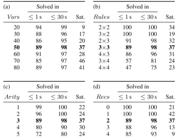
(a) Solved in Vars ≤1s ≤30s Sat. 20 94 99 9 30 88 96 17 40 86 95 20 50 89 98 37 60 91 97 28 70 85 97 46 80 89 97 41 (b) Solved in Rules ≤1s ≤30s Sat. 2×2 100 100 34 3×2 100 100 19 2×3 91 98 32 3×3 89 98 37 4×3 86 96 31 3×4 57 81 24 4×4 47 75 23 (c) Solved in Arity ≤1s ≤30s Sat. 1 99 100 22 2 96 100 24 3 89 98 37 4 80 90 30 5 72 80 24 (d) Solved in Recs ≤1s ≤30s Sat. 0 100 100 21 1 100 100 42 2 89 98 37 3 88 96 13 4 85 93 9

Figure 2. Synthetic benchmark performance of our algorithm.

Proposition 4.16, using a binary adder implementation of the suc-cessor relation. Runtimes, as expected, are exponential inn: cases withn≤4are solved in a fraction of a second, the casen= 5is solved in about half a minute,n= 6takes almost 16 minutes, and

n= 7times out after 40 minutes.

5.2 Benchmarks on automatically abduced predicates Next, we tested our algorithm on a large collection of predicates generated automatically by the CABERtool, which attempts to ab-duce inductively defined safety and/or termination preconditions in our logical fragment for pointer programs [10]. We recorded all candidate preconditions generated by CABERover 29 test pro-grams, including back-tracking attempts. This produced 45 945 syntactically unique inductive rule sets, defining from 1–37 predi-cates with up to 11 parameters and two recursive invocations each. The majority of these definition sets (94%) had no more than 20 predicates; sets with 19 predicates were the most numerous (15%). We found that our algorithm terminates in less than 50 ms on all tests in this suite, and most definition sets (83%) were satisfiable. We believe this is probably due to the relatively simple recursive structure of the predicates produced by CABER.

5.3 Synthetic benchmarks

To evaluate the scalability of our procedure, we generated test cases drawn from a random distribution with parameters:

• Vars: the number of variables inVar;

• Rules=Preds×Cases: the number of predicates and induc-tive rules for each predicate;

• Arity: the arity of all predicates;

• Eqs,Neqs,Points, andRecs: the average numbers of equal-ities, disequalequal-ities, points-to literals, and recursive predicate calls, respectively, in each rule.

Each instance consists ofRules=Preds×Casesindependently generated inductive definitions, with all predicates of the same Arity. On the rule body, the number for each kind of literal is drawn from a Poisson distribution where the parameterλ is set to, respectively,Eqs,Neqs,Points, andRecs. This yields a mix of short and long rule bodies with a specified average length. Furthermore, to have on average one base case for the rule system, with probabilityp= 1/Rulesall the recursive calls in the body of a rule are discarded.

Figure 2 reports our algorithm’s performance on instances drawn from this distribution. Each row collects the results of 100 instances randomly generated with various parameter values; the second and third columns report the number of tests solved in un-der 1 and 30 seconds, while the last one shows the number of solved instances found to be satisfiable. Each of the four sub-tables shows how the statistics vary as one parameter changes while all the rest remain fixed. Although most cases are fairly easy to solve, a few hard instances consistently show up on all parameter settings. For example, with parametersVars= 50,Rules=3×3,Arity = 3, and allEqs,Neqs,Points, andRecsset to 2 (that is the bold line repeated on all four tables), we find that two very hard instances remain unsolved after the 30 s timeout.

6.

Related work

Here we survey the main categories of work related to the contri-bution of this paper.

6.1 Satisfiability in separation logic with inductive predicates Recently, interesting progress has been made on satisfiability and entailment problems in various fragments of separation logic with user-defined inductive predicates as considered here (see Sec-tion 2). In particular, Iosif et al. [20] propose a sub-fragment of our setting, imposing significant syntactic restrictions on the in-ductive definitions to enforce bounded treewidth for all models of a predicate. Here the treewidth of a heaphis determined by a corresponding graph structure. These restrictions allow them to use a reduction to monadic second-order logic (MSO) for their proof that both satisfiability and entailment are decidable in their fragment of separation logic with inductive definitions. However, these syntactic restrictions disallow many natural inductive predi-cates; in particular, predicates describing structures with dangling data pointers, such as list or tree segments with extra arbitrary data fields, or structures where potentially no memory is allocated.1

In this paper, we only consider satisfiability, not entailment (which is undecidable [2]), but we are not restricted to bounded-treewidth predicates. In addition, we provide a direct decision pro-cedure for satisfiability (as opposed to a reduction proof of decid-ability) and contribute an analysis of the complexity of satisfiability checking for our fragment.

Considerable research effort has also been expended on the symbolic heap fragment of separation logic with a list segment predicate only. Berdine et al. [3] provided the first decidability re-sult for satisfiability and entailment in this fragment, with a poly-nomial time procedure given later by Cook et al. [15]. Piskac et al. recently presented another decision procedure, which also works for structures such as sorted list segments and doubly linked lists, based on translating entailments to an intermediate logic that can be handled by an SMT solver [24]. (In very recent work [25], Piskac et al. extended their approach to support also tree-shaped data struc-tures.) Finally, Navarro P´erez and Rybalchenko [22] provided an SMT encoding for satisfiability and entailment in another exten-sion of the fragment allowing pure formulas from arbitrary SMT theories, rather than simple (dis)equalities.

6.2 Satisfiability in other logics with inductive definitions The consistency of inductive predicates defined by first-order Horn clauses has been widely studied in different contexts. One well-known application of such clausal definitions is Datalog, a rule-based query language for relational databases with ties to logic programming. Datalog rules roughly correspond to our inductive rules where the spatial component of rule bodies is alwaysemp.

1_{For further discussion of the limitations of this fragment of separation}

logic we refer to [20].

The evaluation of Datalog queries was shown to be decidable by Shmueli [27] and EXPTIME-complete (see e.g. [16, Theorem 4.5]). However, the interaction between spatial conjunction (∗), allocation (7→) and recursion makes a direct translation to Data-log impractical because it imposes a global constraint; at the same time we found that reducing from Datalog for our lower bounds is possible but no simpler than our circuit-based method.

More recently, Hoder et al. [19] describe a Datalog-based en-gine,µZ, for the fixed point computation of inductive definitions. In contrast to our approach, they compute concrete fixed points based on explicit underlying ground facts (i.e., they focus onmodel checking, as opposed to satisfiability checking).

More generally, there has been some interest from the program analysis and verification community in the satisfiability of Horn and Horn-like clauses. Bjørner et al. [7] advocate such clauses as an interchange format for software model checking tools, while Grebenshchikov et al. [18] describe an abstraction-based procedure for finding models and checking satisfiability of Horn-like clauses in the context of program analysis.

6.3 Separation logic tools with general inductive predicates Several analysis tools based on separation logic allow the user to provide their own inductive definitions for spatial predicates. We have already mentioned in our evaluation (Section 5) the the-orem prover CYCLIST [11], which treats separation logic with user-defined inductive predicates, and the related abductive prover CABER[10], which automatically infers inductive predicate defini-tions as safety/termination precondidefini-tions forwhileprograms. An-other such tool is THOR[21], which proves memory safety and gen-erates sound arithmetic abstractions of heap programs (w.r.t. safety and termination). In THORthe specification and predicate defini-tions must be entered manually. User-defined inductive predicates are also employed in HIP/SLEEK[14], a combined theorem prover and verification system for a C-like language. Finally, the shape analysis in [13] infers inductive definitions based on “structural in-variant checkers” provided by the user.

7.

Conclusion and future work

The decidability status of satisfiability in the symbolic heap frag-ment of separation logic with general inductive predicates has stood open for some time. Following the recent achievement of a partial positive answer to this question in [20], here we resolve the gen-eral case affirmatively. Our decidability proof has the advantage of being constructive: we give a decision procedure for checking the satisfiability of inductively defined predicates and of individual rules defining those predicates.

We show that our satisfiability problem isEXPTIME-complete in the general case, and that it is stillNP-complete when the induc-tive predicates are restricted to at mostk≥3arguments. Despite these high complexities, our experiments indicate that, for predi-cate definitions arising in practice, our prototype implementation is typically able to solve the decision problem in a matter of millisec-onds. This opens up a number of interesting potential applications in the automatic verification of programs based on our fragment of separation logic (which could be used, e.g., to consider heap-based programs employing arbitrary data structures, rather than just lists): • _{First, automatic verification orshape analysisbased on} sepa-ration logic (cf. [4, 5, 12]) typically employs symbolic states based on disjunctions of symbolic heaps. Our algorithm could thus be used to quickly eliminate unsatisfiable disjuncts from symbolic states; it seems plausible that this might yield non-trivial reductions in the time and space costs of such analyses. • Second, although our decision procedure for satisfiability

im-possible in general), it does nevertheless provide a quickpartial

method for proving or disproving such entailments. On the one hand, any entailmentF`Gwith an unsatisfiable antecedentF

is trivially valid. On the other hand,F `Gmust be invalid if the base pairs forF andGimply the existence of a model sat-isfyingFbut notG. To illustrate this point, consider the usual “list segment” predicate of separation logic, defined by

x=y:emp⇒ls(x, y)

x7→z∗ls(z, y)⇒ls(x, y)

Now, consider the (invalid) entailmentls(x, y)`ls(y, x). Com-puting the base pairs for both sides yields

(basels)(x, y) ={(∅,{x=y}),({x},∅)}

(basels)(y, x) ={(∅,{y=x}),({y},∅)}

The second base pair for ls(x, y) implies the existence of a model for ls(x, y) in whichxis allocated andy is not, and hencex6=yin this model. However, the base pairs forls(y, x)

tell us thatymust be allocated in any model ofls(y, x)where

x6=y. That is, there is a model ofls(x, y)that is not a model of ls(y, x). We believe that this sort of reasoning should be quite straightforward to automate.

•Third, our satisfiability procedure can be used to check the san-ity of, and/or remove unsatisfiable clauses from, the definitions of inductive predicates either written by programmers, or in-ferred automatically (cf. [10]).

•_{Finally, beyond deciding the satisfiability of inductive} predi-cates, the set of base pairs computed by our procedure also pro-vides a useful partition of the space to search for models. While Gherghina et al. [17] have shown that a manual case analysis of inductive definitions can guide proof techniques and improve their efficiency; our decision procedure could automate the case analysis required to do so.

Taking a different direction for future work, one could inves-tigate whether our techniques for deciding satisfiability extend to more general variants of separation logic, where general induc-tive predicates are still allowed, but the general format of formulas is less restricted. Possible candidates for such extensions include: higher-order separation logic [6]; the fragment in which formulas may contain pure assertions beyond (dis)equalities [22]; and sepa-ration logic with fractional permissions [8].

Acknowledgements. We wish to thank the anonymous reviewers for their valuable comments, which have helped us greatly in im-proving the presentation of the paper.

References

[1] Satisfiability checker for separation logic with inductive definitions. https://github.com/ngorogiannis/cyclist/releases/ tag/CSL-LICS14.

[2] T. Antonopoulos, N. Gorogiannis, C. Haase, M. Kanovich, and J. Ouaknine. Foundations for decision problems in separation logic with general inductive predicates. InFoSSaCS’14, volume 8412 of

LNCS, pages 411–425, 2014.

[3] J. Berdine, C. Calcagno, and P. W. O’Hearn. A decidable fragment of separation logic. InFSTTCS’04, volume 3328 ofLNCS, pages 97– 109, 2004.

[4] J. Berdine, C. Calcagno, B. Cook, D. Distefano, P. W. O’Hearn, T. Wies, and H. Yang. Shape analysis for composite data structures. InCAV’07, volume 4590 ofLNCS, pages 178–192, 2007.

[5] J. Berdine, B. Cook, and S. Ishtiaq. SLAyer: Memory safety for systems-level code. InCAV’11, volume 6806 ofLNCS, pages 178– 183, 2011.

[6] B. Biering, L. Birkedal, and N. Torp-Smith. BI-hyperdoctrines, higher-order separation logic, and abstraction.ACM TOPLAS, 29(5), 2007.

[7] N. Bjørner, K. McMillan, and A. Rybalchenko. Program verification as satisfiability modulo theories. InSMT’12, pages 3–11, 2012. [8] R. Bornat, C. Calcagno, P. W. O’Hearn, and M. J. Parkinson.

Per-mission accounting in separation logic. InPOPL’05, pages 259–270, 2005.

[9] J. Brotherston. Formalised inductive reasoning in the logic of bunched implications. InSAS’07, volume 4634 ofLNCS, pages 87–103, 2007. [10] J. Brotherston and N. Gorogiannis. Cyclic abduction of induc-tively defined safety and termination preconditions. Technical Report RN/13/14, University College London, 2013.

[11] J. Brotherston, N. Gorogiannis, and R. L. Petersen. A generic cyclic theorem prover. InAPLAS’12, volume 7705 ofLNCS, pages 350–367, 2012.

[12] C. Calcagno, D. Distefano, P. W. O’Hearn, and H. Yang. Composi-tional shape analysis by means of bi-abduction.J. of the ACM, 58(6): 26, 2011.

[13] B.-Y. E. Chang, X. Rival, and G. Necula. Shape analysis with struc-tural invariant checkers. InSAS’07, volume 4634 ofLNCS, pages 384– 401, 2007.

[14] W.-N. Chin, C. David, H. H. Nguyen, and S. Qin. Automated veri-fication of shape, size and bag properties via user-defined predicates in separation logic. Science of Computer Programming, 77(9):1006– 1036, 2012.

[15] B. Cook, C. Haase, J. Ouaknine, M. J. Parkinson, and J. Worrell. Tractable reasoning in a fragment of separation logic. InCONCUR’11, volume 6901 ofLNCS, pages 235–249, 2011.

[16] E. Dantsin, T. Eiter, G. Gottlob, and A. Voronkov. Complexity and expressive power of logic programming. ACM Comput. Surv., 33(3): 374–425, 2001.

[17] C. Gherghina, C. David, S. Qin, and W.-N. Chin. Structured specifica-tions for better verification of heap-manipulating programs. InFM’11, volume 6664 ofLNCS, pages 386–401, 2011.

[18] S. Grebenshchikov, N. P. Lopes, C. Popeea, and A. Rybalchenko. Synthesizing software verifiers from proof rules. InPLDI’12, pages 405–416, 2012.

[19] K. Hoder, N. Bjørner, and L. de Moura. µZ– an efficient engine for fixed points with constraints. InCAV’11, volume 6806 ofLNCS, pages 457–462, 2011.

[20] R. Iosif, A. Rogalewicz, and J. Simacek. The tree width of separation logic with recursive definitions. InCADE’13, volume 7898 ofLNAI, pages 21–38, 2013.

[21] S. Magill, M.-H. Tsai, P. Lee, and Y.-K. Tsay. Automatic numeric abstractions for heap-manipulating programs. InPOPL’10, pages 211–222, 2010.

[22] J. A. Navarro P´erez and A. Rybalchenko. Separation logic modulo theories. InAPLAS’13, volume 8301 ofLNCS, pages 90–106, 2013. [23] C. H. Papadimitriou and M. Yannakakis. A note on succinct

represen-tations of graphs.Inf. Control, 71(3):181–185, Dec. 1986.

[24] R. Piskac, T. Wies, and D. Zufferey. Automating separation logic using SMT. InCAV’13, volume 8044 ofLNCS, pages 773–789, 2013. [25] R. Piskac, T. Wies, and D. Zufferey. Enabling automated reasoning

about separation logic of trees with data. InCAV’14, 2014. To appear. [26] J. C. Reynolds. Separation logic: A logic for shared mutable data

structures. InLICS’02, pages 55–74, 2002.

[27] O. Shmueli. Decidability and expressiveness aspects of logic queries. InPODS’87, pages 237–249, 1987.

[28] H. Yang, O. Lee, J. Berdine, C. Calcagno, B. Cook, D. Distefano, and P. O’Hearn. Scalable shape analysis for systems code. InCAV’08, volume 5123 ofLNCS, pages 385–398, 2008.