Planning Multi-Modal Transportation Problems

(1)

Planning Multi-Modal Transportation Problems

Jos´e E. Fl´orez

[email protected]

´

´

Angel Garc´ıa-Olaya

[email protected]

Daniel Borrajo

[email protected]

Computer Science Department, Universidad Carlos III de Madrid Avenida de la Universidad 30, 28911 Legan´es, Madrid, Spain

Abstract

Multi-modal transportation is a logistics problem in which a set of goods have to be transported to different places, with the combination of at least two modes of transport, without a change of container for the goods. The goal of this paper is to describeTIMIPLAN, a system that solves multi-modal transportation problems in the context of a project for a big company. In this paper, we combine Linear Programming (LP) with automated planning techniques in order to obtain good quality solutions. The direct use of classical LP tech-niques is difficult in this domain, because of the non-linearity of the optimization function and constraints; and planning al-gorithms cannot deal with the entire problem due to the large number of resources involved. We propose a new hybrid algo-rithm, combining LP and planning to tackle the multi-modal transportation problem, exploiting the benefits of both kinds of techniques. The system also integrates an execution com-ponent that monitors the execution, keeping track of failures and replans if necessary, maintaining most of the plan in exe-cution. We also present some experimental results that show the performance of the system.

Introduction

Since the logistics domain was defined (Veloso 1992), logis-tics problems have been traditionally used by planning prac-titioners to show the performance of their systems. It was a simplified version of a real problem, which represents an im-portant task for companies that have to transport many goods among different places. In this paper, we describe the work we have done on trying to apply current automated planning techniques to solving a real logistics problem. In our case, we deal with multi-modal transportation, that is character-ized by the combination of at least two modes of movement of goods, such as road, rail, or sea (Muller 1999). The de-velopment of multi-modal transportation has been followed by an increase in multi-modal transportation research —see e.g. (Macharis and Bontekoning 2004). Thus, it provides a real and challenging domain for researchers working on Artificial Intelligence (AI) planning and scheduling.

ever, there are relatively few applications to solve the multi-modal transportation problem. The logistics research usu-ally focus on only one mode of movement of goods, whether by road (Ropke and Pisinger 2006), rail (Salido and Bar-ber 2009) or sea (Imai, Shintani, and Papadimitriou 2009). Multi-modal transportation is more complex than the uni-modal one. Beyond the obvious remark that multi-uni-modal transportation problems induce state spaces which are or-ders of magnitude larger than the state space of each partic-ular uni-modal transportation problem, there are two obser-vations that make multi-modal transportation problems quite challenging: on one hand, the optimal path is not the short-est path anymore; instead, additional costs have to be con-sidered at the nodes where a new transpotation mean is ap-plicable —e.g., money and/or time. On the other hand, a new class of constraints has to be observed which (to make things harder) is dependant on each node —e.g., operat-ing an exchange of transportation mean can actually involve other subproblems as it happens when moving freights from a truck to a ship.

In this paper, we deal with a real-world problem and in par-ticular we focus on intermodal freight transport. Our con-tribution attempts to provide a new application,TIMIPLAN, to solve problems of this kind. The planning component of TIMIPLANconsists of two phases: in phase one, for each set of goods to be picked up and delivered, the containers and trucks with minimum estimated cost to complete the service are selected. In this phase, several assignment models are constructed and solved as linear programming problems. In phase two, an AI planner is used to select the best (cheapest) plan to serve each service: from a first pick-up point to the last delivery point over the transportation route. The plan should fulfill a given set of constraints (temporal and regu-latory), and will include the sequence of the transportation modes to be used. Although some of the application areas addressed in AI and Operations Research (OR) are very sim-ilar (e.g., planning, scheduling), the methods that are used to solve these problems are substantially different. In this paper, we describe the application we have developed for a big logistics company, discuss the difficulties on using “as is” current AI planning technology for solving this task, and provide some experimental results that evaluate the software in real situations extracted from the customer database. Proceedings of the Twenty-First International Conference on Automated Planning and Scheduling

(2)

The remainder of this paper is organized as follows. Section

Related Work gives a brief summary of the transportation problem in its uni-modal and multi-modal versions, intro-ducing some of the main approaches used to solve it. Sec-tionProblem Descriptiondescribes the multi-modal trans-port problem. SectionTIMIPLAN presents theTIMIPLAN application. SectionEvaluationincludes experiments rela-tive to the algorithms used in TIMIPLAN. Lastly, Section

Conclusionspresents the conclusions and further research.

Related Work

There have been already many approaches that deal with the uni-modal transport problem. An overview can be found in (Nanry and Wesley Barnes 2000). In the multi-modal transport problem there has also been some work done, though none of these works solves the complete logistics problem, being centered in other problems associated with multi-modal transportation or in subproblems that do not represent all the constraints. In (Macharis and Bontekon-ing 2004), the authors discuss the opportunities for OR in intermodal freight transport. The paper reviews OR mod-els that are currently used in this emerging transportation research field and defines the modeling problems which need to be addressed. In (Eibl, Mackenzie, and Kidner 1994), the authors present a case study applying an inter-active vehicle routing and scheduling software to a brew-ing company in the UK. They explain how a commercial tool was applied to schedule the day-by-day (operational) vehicle routing and scheduling to distribute the goods. This tool was specific for the brewing problem, and the opera-tor that manages the tool needs a previous training process to manage all variables involved. In our case, the solution is quite domain-independent, with less user knowledge re-quirements. In (Catalani 2003), a statistical study is pre-sented to improve the intermodal freight transport through Italy, by using the road-ship and road-train transports. In this study, only the main points of origin or destination are taken into account, so the study does not deal with the complete network complexity problem, as we do. In (Qu and Chen 2008), the authors pose the multi-modal transport problem as a Multicriteria Decision Making Process (MCDM). They propose a hybrid MCDM by combining a Feed-forward Ar-tificial Neuronal Network with a Fuzzy Analytic Hierarchy Process. The case study is a network in which nodes repre-sent terminals, and edges reprerepre-sent different transportation modes (road, ship and train). The model can deal with sev-eral cost functions and constraints, but they only define six nodes, while our maps can have thousands of nodes.

Problem Description

We define a logistics problem as the tuple < G, F, C, R, B, S > where G is the network graph, F, C, R and B are the sets of trucks, containers, trains and ships respectively and S the services that should be

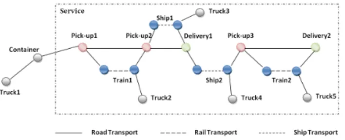
fulfilled. The nodes inGrepresent the locations where the goods should be picked up or delivered. A services ∈ S specifies pickup and delivery operations, each one with a location and service time, that indicates the time at which the corresponding location is available for the pick-up or the time at which a delivery service should be performed. To complete a service only a containerc∈Cis required, but it can be moved by using a combination of vehicles: trucks, trains and/or ships. Each truck t ∈ F has information relative to the location and time at which it will be available and its corresponding driver’s accumulated driving time. If a truck is used, it should travel to pick the container up, and either visit all locations of the transportation request (pick up and delivery locations), or transport it to the next transportation means (train station or port), where the rest of the plan might involve one or several other transportation vehicles. Trains and ships have a timetable specifying their movement actions and the load and unload actions can only be executed when they are in a station/port. The resulting plan should satisfy the given service times of the locations. For instance, if the truck and container arrive early, they have to wait at the location until it is available. If the truck and container arrive late, there will be a cost penalty. In multi-modal transportation, several trucks are usually needed. For example, Figure 1 shows how, in order to com-plete the service, there are five available trucks, one tainer, two trains and two ships. The first truck with the con-tainer picks the shipment up fromPick–Up1and transports

it toPick–Up2using either road or train. If the train option

is selected, another truck will be necessary to transport the container toPick–Up2. Also, there are two other decision

points related to the use of Ship1andTrain2. The use of

Ship2andTruck4is mandatory for reaching thePick–Up3

point.

Figure 1: Example of multi-modal transportation graph.

Thus, there are several kinds of resources, each one with different kinds of costs (e.g., moving the truck empty is dif-ferent from moving it loaded), difdif-ferent routes (either single mode routes, as all road, or multi-modal routes, as combin-ing trucks with barge and/or rail), and with temporal and resource constraints (drivers have constraints on number of continuous driving hours, for instance). Several constraints have not been included in the previous description of the problem, due to the difficulty of formalizing them or be-cause they depend on information that is not available in

(3)

the system. For example, there are soft goals related to the places where the drivers prefer to stop or to the client’s pref-erences about vehicles and/or containers used to transport their goods. Also, human planners have expert knowledge about the probabilities of new services arising in each zone. They use that knowledge to reserve trucks or containers in these zones or make movements that prepare all resources for future unknown services. Given that it is impossible to predict all potential soft goals to be taken into account when planning, we use a mixed-initiative approach to help the user taking into account those constraints that cannot be easily handled byTIMIPLAN.

The planner is executed every day. A daily problem has approximately 600 locations (summing up all pick-up and delivery locations, as well as initial positions of trucks, con-tainers, ships, and trains), 175,000 edges among those lo-cations, 300 trucks, 300 containers, 300 services, 50 train segments and 150 ship segments. The company imposes a time limit of 2 hours for computing the daily plan.

TIMIPlan

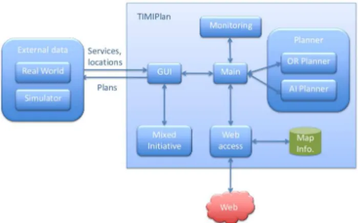
TIMIPLANsolves logistics multi-modal problems. In a plan-ning context, it receives the positions of the set of all avail-able resources as input (initial state), a number of services to be performed (goals) and has to generate a plan with actions including: the load of goods in different places; the unload on others; and the assignment and movement of the available resources (trucks, containers, ships, trains, . . . ) to complete this request. Also, it must take into account several con-straints, such as pick-up and delivery times. The objective is to minimize the cost of servicing all the daily requests. TIMIPLANis composed of a set of modules as shown in Fig-ure 2. The input is the list of services to accomplish and the list of available resources (initial locations of each resource, costs, constraints, . . . ), both in XML format. The output is a plan for each service. This plan can be graphically inspected on a map which includes points where the actions are per-formed and the routes followed by the vehicles. The Web access component performs different queries to Web portals like Google Maps, postal codes services or traffic informa-tion. The main module fuses all the gathered data to gen-erate the problem description and delegates the work to the planning and monitoring modules. OnceTIMIPLANcreates the problem description, it is passed to the planner (com-bination of OR and AI). The Monitoring component allows TIMIPLANto detect deviations from the original plan, or new services to be planned for, that arise everyday and triggers replanning when necessary.

For a full integration with the company’s information sys-tems,TIMIPLANhas to support two modes of operation: of-fline and online. The ofof-fline mode runs everyday to gener-ate the next day’s planning. In the online mode, the system monitors the position of each resource, the execution of

ac-Figure 2:TIMIPLANarchitecture.

tions and the replanning when necessary. The system also incorporates a simulator that allows the analysis of potential plan alternatives generated by the user. The mixed initiative module allows the human experts to interact withTIMIPLAN in order to include extra information in the problem, plan to consider the constraints and goals that cannot be formalized explicitly, or solve unexpected failures.

Planning module

The first approach we followed consisted on trying to solve the complete problem by using an automated planner. Un-fortunately, given the size of the problem, no domain-independent planner can go beyond the initial instantiation phase. For instance, theload-truck_{action has three} pa-rameters (truck, container, location). In our problems, we deal with around 300 trucks and containers, and around 600 locations. Thus, there are about300×300×600 = 54

million potential instantiations of that action solely. One po-tential way of solving the instantiation problem could be to model all trucks in a uniform way. So, one could define at each location the number of trucks at that location. Thus, moving a truck from one location to another would only con-sider the two locations, and the effect would be to add one to the destination location and subtract one from the source lo-cation. However, this solution requires all trucks to be equal. In our case, each truck is different given that drivers, who are assigned to trucks by the company (and this assignment cannot be controlled), have different properties, mainly re-lated to the regulations (number of continuous driving hours, number of rest hours, and so on). Also, these regulations are different depending on the location. In a similar way, linear programming experiences a combinatorial explosion due to the huge number of resources involved.

First, we compute the assignment of trucks and containers to services taking into account the initial positions of the trucks and containers, using a LP approach. Then, our ap-proach sequentially solves the problem, using three different

(4)

steps for each service. In step one, the container and truck/s with minimum cost estimated to complete the service are selected. In step two, a planning module is used to select thebest path from a first pick-up point to the last delivery point over the transportation route. In this case,bestmeans that the path fulfills the given set of constraints, including the sequence of the transportation modes used (where sev-eral trains and/or ships can be used) with the minimum cost. This two-step approach balances the total cost obtained and the time required to compute the plan. The high level algo-rithm has been depicted in Table 1. The network graph is the graph defined by the locations (pick-up and delivery nodes, positions of trucks, containers, train stations and ports) and edges (roads, rails and ship lines). In step three, we update the assignment of trucks and containers to services taking into account the final position of the trucks and containers used to complete the last planned service. In the third step, we use the same LP approach again.

TIMIPLAN(G, F, C, R, B, S): plan

;; Inputs: the graph (G), the set of trucks (F), containers (C), trains (R), ships (B) and services (S)

plan=_∅

;; Compute the initial assignment of trucks and containers to services (A)

A=solveAssignmentProblem(G, F, C, R, B, S) For eachs∈S

;; Select the truck/s and container to complete the service

selectedTrucks,selectedContainer= getServiceAssigment(A, s)

;; Plan the service with the truck/s and container selected. Select the best transportation modes

plan=_{∪ {solvePlanningProblem}(selectedTrucks, selectedContainer, R, B, s)}

;; Updates assignment with the new cost of selectedTrucks and selectedContainer

A=updateAssignmentProblem(G, F, C, R, B, S) Returnplan

Table 1: Top level algorithm ofTIMIPLAN.

There are several reasons that make the use of LP diffi-cult to solve the second subproblem (the selection of the best transportation modes for each transportation request), and advocate the use of other techniques as automated plan-ning. Multi-modal transportation problems are non-linear in the constraints (e.g. the limits for when and how long truck drivers may drive and rest), and in the objective func-tion (e.g. the cost for delayed delivery depends non lin-early on the amount of delayed time). Though there are some works that transform non-linear problems into linear ones using techniques involving piecewise linear approxi-mation (Turkay and Grossmann 1996), or other transform-ing methods (Wang, Chukova, and Lai 2005), they usu-ally involve the inclusion of additional constraints or vari-ables, complicating excessively the model. For a quadratic problem withn 0-1 variables, Oral-Kettani’s method (Oral and Kettani 1992) (considered as one of the most efficient linearization technique published) would introducen addi-tional continuous variables andnauxiliary constraints, and for a cubic problem with n 0-1 variables, Oral-Kettani’s method would introduce3nadditional continuous variables and3nauxiliary constraints. Furthermore, if we decide to use non-linear programming to solve the problem, no gen-eral method exists for solving non-linear programming

prob-lems (NLP) in the same manner as the Simplex method solves LP problems. Moreover, the number of resources and temporal constraints involved preclude the use of an-alytical (optimal) procedures, as LP, to solve these prob-lems (Church et al. 1996). In this case, LP exceeds the time limit of two hours to solve a daily problem. So, it is necessary to use heuristic search methods in order to ob-tain good quality (but sub-optimal) solutions. In addition, planning actually starts by considering a very expressive language which usually overcomes some of the difficulties found when modeling a problem with linear constraints and non-linear optimization functions.

Assignment Problem In the classical assignment

prob-lem, the goal is to find an optimal (minimum cost) as-signment of resources to tasks taking into account the con-straints, and ensuring that all tasks are completed. In Fig-ure 1, a service with three pick-up points and two deliv-ery points is shown. It is possible to use either the road or the railway betweenPick–Up1andPick–Up2and between

Pick–Up3andDelivery2. Also, it is possible to use the road

or a ship betweenPick–Up2andDelivery1and only a ship

betweenDelivery1 andPick–Up3. If multi-modal modes

are selected to solve the service, trucks Truck2_, _Truck3_,

Truck4 _and_Truck5 _{pick the container up from the}

desti-nation port or station and continue the transportation route until they reach the next origin port, station or the final de-livery node. Given the size of the whole assignment prob-lem, we decompose it into three subproblems: assignment of containers to trucks, assignment of trucks and containers to services, and assignment of trucks to multi-modal nodes. In all these subproblems the objective criteria is to minimize a function cost. There are no additional constraints to those imposed by the assignment problem itself, i.e. each resource cannot be assigned to more than one task and viceversa. In the first subproblem, we solve the assignment of empty containers to trucks. The cost of a truck-container assign-ment is estimated taking into account the distance between them, the time at which they will be available and the transportation cost of each truck. In the second subprob-lem, we solve the assignment of trucks with containers to services, using the assignments computed in the previous phase. These operations involve the provision of an empty truck and container to the service. The truck and container are used in the subsequent transportation until they arrive to the last delivery point in the service or until they arrive to a multi-modal node in the transportation route. To estimate the assignment cost, we consider the position and time of both the service and the truck with container. In multi-modal transportation, additional trucks are needed in order to com-plete a service. These trucks pick-up the containers from the destination station/port and transport it to complete the ser-vice, or until they arrive to the next multi-modal node. So in the third assignment subproblem, the method selects the best truck to pick-up the container from the destination sta-tion/port and continue the transportation route. It takes into account again the previous assignments. Like in the previous

(5)

subproblems, we take into account the position and avail-ability time of each truck in comparison with the estimated time at which the container will arrive to the multi-modal node.

The system can deal with different number of services, trucks and containers. Indeed, the usual scenario is to have more trucks and containers than services, and more contain-ers than trucks. In case that there were more services than trucks/containers, the system will assign the same truck to several services. Since the services are sequentially solved, each time a service is planned we update the position and availability time of all the resources involved. Thus, in the next step, the assignment problems will take into account the new values when estimating assignment costs.

Planning Problem One of the inputs of the planning

pro-cess is the list of truck/s and container selected by the as-signment process for each service. A planning problem is built for each service and the planner must select the best transportation modes to complete it. Moreover, the planner must schedule each pick-up and delivery according to the constraints. First, it selects the trains and ships that can po-tentially be used to complete the transportation route. Then, the planning problem is constructed taking into account the trains, ships and the truck/s and container selected to com-plete the transportation route. This planning task has several features that make it very hard for current planners.

• Time management: _{The existing temporal restrictions}

in the problem (each pick-up and delivery is scheduled according to the time service of each location) imply that we need an explicit management of the current time. If a truck arrived early to a pick-up or delivery point, it must wait, and when it arrives later, a penalty cost is applied. In addition, a container must wait at stations and ports for the next departure of the train or ship. We use fluents to define and handle the temporal aspect.

• _{Management of functions:} _{In this domain, we use a}

large number of functions. Some examples are: cost per kilometer when truck travels with/without a container, time spent loading/unloading a container in a train or ship, or time spent by a train or ship to go from a location to another. In addition, other functions are used to limit the driving and resting times of drivers.

• Locations: TIMIPLAN should indicate how to go from

one place to another, so information about the transporta-tion map should be added to the problem descriptransporta-tion in-cluding distances, and cost per edge.

Some of these features can be handled by some temporal planners. However, there are currently only a few that can also support functions, and metrics, as needed in this project. In our work, instead of using a temporal planner, we use a planner that augments the Metric-FF planner (Hoffmann 2001) with some representation features (computation of

costs that depend on non-static components of the state). We use A∗as the search algorithm.

Mixed Initiative

TIMIPLANimplements a fully planning process that allows the user, once the services are complete and the available resources are provided, to automatically obtain a complete plan. That plan takes into account most of the constraints, but not all because some cannot be represented and effi-ciently handled by the system. For example, drivers prefer services near home or prefer to work only on week days. In addition, several failures may occur once the services are planned, which are fixed by humans in real time through phone calls. Finally, human experts are usually suspicious of tools that provide solutions which cannot be changed, regardless of how sophisticated or intelligent the tool is. Thus, a mixed-initiative component has been implemented to allow the human planners to modify the plans provided by TIMIPLAN, according to their suggestions made during the project. Currently, they can change means of transport, such as trucks, containers or ships, and change the order of pickup and delivery operations. These changes are per-formed through the GUI, that also propagates the effects of these changes: whether the plan is still valid (does not vio-late any constraint) and what is its new cost.

Monitoring and Replanning

The monitoring component checks whether the execution of the plan is deviating from the expected and triggers replan-ning if needed. Given that we are dealing with a real-time system, with a large number of resources involved, it is not possible to replan from scratch. So, our replanning compo-nent consists on adapting the existing plan to the new state, aiming to perturb the original plan as little as possible (also known asplan repair(Fox et al. 2006)). We consider three kinds of situations that may occur during the monitoring pro-cess: damaged trucks, new services, and traffic jams.

• _{Damaged trucks:} _{In this case, only the services}

associ-ated with the damaged truck are replanned (i.e. only a part of the original plan is modified). The replanning process is composed of two different steps: assignmentof a new truck to replace the damaged truck, andplanningof the new transportation modes to complete the service. The as-signment process selects the truck to replace the damaged truck following a fully greedy strategy, (select the truck with the least estimated cost, taking into account if it is associated with a previous service or not, its localization, if it is engaged with a container or not). The new selected truck drives to the damaged truck, picks the container up and continues the transportation route. If the damaged truck was associated with more services, a new truck is selected to replace it in each of them. The new times and action costs are propagated throughout the plan.

(6)

• New services:_{In this case,}TIMIPLANproceeds in a sim-ilar way as previously; first, anassignmentof truck/s to complete the service, and thenplanningof the best trans-portation modes to complete it. The truck/s are selected following a fully greedy strategy, and only these trucks are considered for the planning problem. The actions planned to solve the new service are added to the original plan, with its corresponding action times and costs.

• _{Traffic jams:} _{Traffic jams increase the duration of}

ac-tions related to trucks movements. These situaac-tions may occur at any moment during the monitoring process. If a truck is delayed due to a traffic jam, TIMIPLAN moni-tors it, propagating the delay to all the actions that depend on that truck (in the same service or in others using that truck), computing the new time and plan cost. If the de-lays create a constraint violationTIMIPLANalerts the user and s/he decides if replanning is neccesary.

If some other unexpected situation arises during the moni-toring process, this module delegates on the mixed-initiative component, allowing the human experts to solve it.

Empirical Evaluation of

TIMIPLAN This section presents the evaluation of the two main com-ponents of TIMIPLAN: the planning, and monitoring and replanning modules. To evaluate the TIMIPLAN planning module, we use a set of representative problems, based on the real data gathered by the company. The problems were generated using ship routes and pick-up and delivery points gathered from real problems. There has been a positive qual-itative evaluation from users. However, direct comparison against the current solutions adopted by Acciona are not pos-sible at this point. First, their databases are handled by hu-mans, so even if they have many inconsistencies (bad written addresses, same company with different names, ...), humans are able to live with those inconsistencies, while planners need the data to be error free. Second, our application was developed by the central offices to address the loss of solu-tions quality due to the decentralized planning (resources) among the branches, as it is currently done. Thus, currently there is no human solving a 300 services assignment (each branch considers instead a smaller problem). There are no plans of such size to compare against, and also coming up with a plan for 300 services is a hard task for humans. How-ever, they already examined the generated plans and consid-ered them to be in the range they would generate.

Two versions of theTIMIPLAN algorithm are used to solve problems of different sizes. Both versions differ on how they perform the first step of the algorithm: the assignment of truck/s and container to services. The first algorithm was explained in Section (we will call it TIMIPLAN (LP)). In this algorithm, LP techniques are used to solve the assign-ment of truck/s and containers to services. In the second ver-sion of the algorithm, a greedy approach is used to select at each step the container and truck/s with the least estimated

cost for each service (TIMIPLAN (Greedy)). In this case, no cost matrix is built as in the TIMIPLAN(LP) algorithm, selecting greedily for each service the truck and container with the least estimated cost. We define ten types of prob-lems in ascending order of size. Each problem has a linear increase in the number of services (between 75 and 300), nodes (between 150 and 600), trucks (between 75 and 300), containers (between 75 and 300), ships segments (between 60 and 150) and train segments (between 5 and 50). For each problem size, ten different problems are solved in order to obtain representative mean values and standard deviations. Given that the company started mainly as a ship transporta-tion company, all problems contain locatransporta-tions on islands, so it is necessary to use ships. Figure 3 shows graphically the comparison of mean times to solve problems of the differ-ent types using the two differdiffer-ent versions of theTIMIPLAN algorithm. The experiments were conducted on a 2,4 GHz quadcore processor with 4 GB RAM, running Linux.

Figure 3: Mean solving time and standard deviations.

The solid red line shows the mean times and standard de-viations spent by the TIMIPLAN algorithm when using LP. The dashed blue line shows the mean times and standard deviations needed by theTIMIPLANalgorithm when it uses the greedy strategy. In the case ofTIMIPLAN(LP), the mean time grows from 65 seconds (the mean timeTIMIPLANtakes to solve the simplest problem) to 6896 seconds (mean time it takes to solve the most complex problem). Given that it performs a more complex assignment of trucks and contain-ers to routes, this vcontain-ersion of theTIMIPLANalgorithm needs more time to solve problems than the greedy approach. In the latter, the mean time ranges from 38 seconds to 3237 seconds. In both cases, time grows exponentially, but the curve is less steep in the case ofTIMIPLAN(Greedy). Given that the time limit for solving the real problems was set to two hours (7200 seconds), TIMIPLAN is able to cope with those hard problems within the allotted time limit.

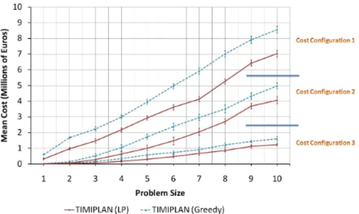
In order to analyze the sensitivity of both solutions to the costs defined by the company, we studied three different cost configurations, ordered in decreasing order of cost (costs of configuration 1 are higher than those of configuration 3).

(7)

Each cost configuration is composed of: a cost per kilometer when trucks travel without any container or the container is empty, a cost per kilometer when trucks travel with container and are loaded, a cost per hour when trucks are stopped in a location, a penalty cost per hour applied when a delivery is delayed, and a penalty cost per hour applied when a pick-up is delayed. Again, these cost settings are based on the real data gathered from the company. Figure 4 shows the comparison of quality (cost) of solutions of the same prob-lems solved previously using the three cost configurations. In Figure 4, the costs are expressed in millions of euros. In this case, the solid red line labeled as TIMIPLAN (LP)

shows the mean costs and standard deviations obtained by theTIMIPLANalgorithm when it uses LP, while the dashed blue line showsTIMIPLAN(Greedy)behavior. In all cases, the mean cost obtained byTIMIPLAN (LP)is less than the cost obtained by the greedy approach.

Figure 4: Mean costs (in million euros) and standard devia-tions for the three proposed cost configuradevia-tions.

The difference in costs between the LP and Greedy ver-sions depends on the cost configuration. So, for instance, in cost configuration 1, the solution byTIMIPLAN(LP)for the problem of type 10 is approximately 1.53 millions of euros cheaper than the solution obtained by the greedy approach. Given these results, when higher cost penalties are used, the differences in the total cost (quality) between the LP and

Greedyplans are more significant. TheLPapproach always presents a cost saving (higher quality) over theGreedy ap-proach. Given that the main driver of the company is the re-duction in cost, once the rest of constraints are fulfilled, the combined approach of OR and AI techniques can be deemed as the best current option.

In order to evaluate theTIMIPLAN monitoring and replan-ning module, we analyzed the time required to replan a dif-ferent number of damaged trucks and new services (Fig-ure 5). Previous to the monitoring and replanning process, a plan is built for attending the daily services (we are consider-ing a daily problem composed of 68 services, 90 trucks, 100 containers, and 7 ships). Thisoriginalplan is a good guide to rebuild a new plan when new situations occur (damaged

trucks or new services that may appear during the day). Fig-ure 5 shows in thex-axisthe number of damaged trucks or new services and in they-axisthe time spent by the replan-ning process.

Figure 5: Mean time (in seconds) spent by the replanning process for a different number of damaged trucks or new services.

Replanning damaged trucks is more time demanding than replanning new services. Replanning damaged trucks re-quires propagating the new time and cost throughout the plan and replacing it in all the services where it appears. Replanning new services only requires inserting additional actions to the plan. However, the replanning process is able to deal successfully with the daily damaged trucks and new services of the company. Rarely 25 trucks could be dam-aged within a day (at least at the same time), or 25 new services are replanned at the same time (normally, they are received scattered throughout the day). Nevertheless, these experiments show that theTIMIPLANreplanning algorithm behaves successfully in these extreme situations.

Conclusions

In this paper, we have introducedTIMIPLAN that success-fully solves big multi-modal transportation tasks. Multi-modal transportation usually involves the combination of a large number of resources, together with temporal con-straints, resource consumption, cost functions, etc. Clearly the bottleneck in this problem is the combinatorial explosion which makes obtaining optimal solutions impossible in the time limit established by the company using only classical planning or only OR techniques. Given the problem’s size, existing domain-independent planners cannot solve those in a reasonable time. Instead, we decompose the problem into two different subproblems. In the first one, we compute the assignment cost of resources (trucks and containers) to tasks (services). In the second one, we formulate each task as a planning problem where different actions are taken (se-lecting the best transportation modes) to achieve the goals

(8)

(the different pick-up and delivery requests for each service) taking into account the resources (trucks and containers) se-lected in the previous phase. LP has shown to be effective to optimally solve the different assignment subproblems, and automated planning has solved successfully the selection of the best transportation modes. This novel way of combining linear programming and planning has allowed us to balance the total cost (quality) obtained, the time required to com-pute a solution and the time to model the different optimiza-tion problems.

Another key issue in relation to solving real world problems consists on the difficulty of modelling. In our case, we could have opted to spend much more time on modelling the whole problem as a LP or CSP problem, or to spend much more time on coming up with a solution to the grounding explo-sion problem for current planners. It might be possible that following those alternatives would have generated a better solution in terms of quality and/or time. We believe that our current solution is a viable solution that has also mini-mized the modelling time (programming effort) providing a good solution to the task. As a side effect, we have also separated the modelling difficulties, so that we deal with the best solution in terms of the multiple criteria problem of <modelling time, quality of solution, time to solve>. Empirical evaluation shows that this combination of tech-niques finds valid plans to complete all the daily services of the company within the imposed time limit, and outper-forming the quality of plans obtained by a reasonable sim-pler approach. Besides, the replanning approach has suc-cessfully dealt with a large number of damaged trucks and new services. TIMIPLANprovides several improvements to the company operations. Currently, both the assignment of resources and the route specification are generated manually by human experts who work in different places, each one having a local view of the overall problem so that they can only handle their own resources.

In order to finally deploy TIMIPLAN we have to clean the databases (or include some kind of robust input parsing), and setting up GPS on both trucks and containers for monitoring and replanning. As future work, we consider combining LP and automated planning in a different way to find better so-lutions (lower cost) in less time.

Acknowledgements

This work has been partially supported by the TIMI (CENIT Spanish R&D collaborative projects with industry) and TIN2008-06701-C03-03 projects. We would like to thank the people from Acciona.

References

Catalani, M. 2003. Transport Competition on a Multimodal Corridor by Elasticity Evaluation.

Church, R. L.; Church, R. L.; Sorensen, P.; and Sorensen, P. 1996. Integrating normative location models into gis: prob-lems and prospects with the p-median model. InP. Longley y M. Batty: Spatial Analysis: Modelling in a GIS environment Cambridge, Geoinformation international.

Eibl, P.; Mackenzie, R.; and Kidner, D. 1994. Vehicle Rout-ing and SchedulRout-ing in the BrewRout-ing Industry. International Journal of Physical Distributioin and Logistic Management

24(6):27–37.

Fox, M.; Gerevini, A.; Long, D.; and Serina, I. 2006. Plan stability: Replanning versus plan repair. InIn Proc. ICAPS, 212–221. AAAI Press.

Hoffmann, J. 2001. FF: The Fast-Forward Planning System.

AI Magazine22(3):57–62.

Imai, A.; Shintani, K.; and Papadimitriou, S. 2009. Multi-port versus Hub-and-Spoke Port calls by Containerships.

Transportation Research Part E: Logistics and Transporta-tion Review.

Macharis, C., and Bontekoning, Y. M. 2004. Opportunities for OR in Intermodal Freight Transport Research: a Review.

European Journal of Operational Research153:400–416. Muller, G. 1999. Intermodal Freight Transportation. Wash-ington DC, USA: Eno Transportation Foundation, Inc. Nanry, W. P., and Wesley Barnes, J. 2000. Solving the Pickup and Delivery Problem with Time Windows Using Reactive Tabu Search. Transportation Research Part B: Methodological34(2):107–121.

Oral, M., and Kettani, O. 1992. A Linearization Procedure for Quadratic and Cubic Mixed-Integer Problem. In Opera-tions Research, 109–116.

Qu, L., and Chen, Y. 2008. A Hybrid MCDM Method for Route Selection of Multimodal Transportation Network. InISNN ’08: Proceedings of the 5th international sympo-sium on Neural Networks, 374–383. Berlin, Heidelberg: Springer-Verlag.

Ropke, S., and Pisinger, D. 2006. An Adaptive Large Neighborhood Search Heuristic for the Pickup and Deliv-ery Problem with Time Windows. Transportation Science

40(4):455–472.

Salido, M. A., and Barber, F. 2009. Mathematical Solutions for Solving Periodic Railway Transportation.Mathematical Problems in Engineering.

Turkay, M., and Grossmann, I. E. 1996. Disjunctive programming techniques for the optimization of process systems with discontinuous investment costs-multiple size regions. Industrial & Engineering Chemistry Research

35(8):2611–2623.

Veloso, M. M. M. A. 1992.Learning by analogical reason-ing in general problem-solvreason-ing. Ph.D. Dissertation, Pitts-burgh, PA, USA. UMI Order No. GAX92-38831.

Wang, D. Q.; Chukova, S.; and Lai, C. D. 2005. Reduc-ing quadratic programmReduc-ing problem to regression problem: Stepwise algorithm. European Journal of Operational Re-search164(1):79–88.

Planning Multi-Modal Transportation Problems