Forecasting for Inventory Control with Exponential Smoothing.

(1)

ISSN 1440-771X ISBN 0 7326 1065 6

M O N A S H U N I V E R S I T Y

AUSTRALIA

Forecasting for Inventory Control with Exponential Smoothing

Ralph D. Snyder, Anne Koehler and Keith Ord

Working Paper 10/99

August 1999

DEPARTMENT OF ECONOMETRICS

AND BUSINESS STATISTICS

(2)

Forecasting for Inventory Control with Exponential Smoothing

Associate Professor Ralph D. Snyder

Department of Econometrics and Business Statistics Monash University

Clayton, Victoria 3168 Australia

Professor Anne Koehler

Department of Decision Sciences Miami University

Oxford, OH45056, USA Professor Keith Ord

Department of Management Science The Pennsylvania State University University Park, PA 16802, USA

(After July 1, 1999: McDonough School of Business, Georgetown University, Washington, DC 20057 USA)

Abstract:

Exponential smoothing, often used for sales forecasting in inventory control, has always been rationalized in terms of statistical models that possess errors with constant variances. It is shown in this paper that exponential smoothing remains the appropriate approach under more general conditions where the variances are allowed to grow and contract with corresponding movements in the underlying level. The implications for estimation and prediction are

explored. In particular the problem of finding the prediction distribution of aggregate lead-time demand for use in inventory control calculations is considered. It is found that unless a drift term is added to simple exponential smoothing, the prediction distribution is largely unaffected by the variance assumption. A method for establishing order-up-to levels and reorder levels directly from the simulated prediction distributions is also proposed.

Key Words: Inventory control, demand forecasting, exponential smoothing, bootstrap

(3)

1. INTRODUCTION

The conceptualisation of simple exponential smoothing (Brown, 1959) was an important

development for demand forecasting in inventory control. Yet implementations of this method

have often been surrounded by practices, summarised in Gardner(1985), which possess

questionable theoretical roots and which, at best, have enjoyed a mixed success. This paper is

written on the assumption that good practice emerges from sound theory and that such a

strategy must be built on the statistical models underlying the technique. Our contribution is

to suggest that the theory of simple exponential smoothing can be extended to a broader class

of models where error variances, instead of remaining constant, can change over time. The

implications of this heteroscedasticity for estimation are explored in section 3. Its

consequences for prediction, particularly in relation to aggregate lead time demand, a quantity

of particular interest in inventory control, are outlined in section 4.

In a recent paper (Ord, Koehler and Snyder, 1997) the methods of exponential smoothing

were shown to apply under much more general conditions than those traditionally envisaged

in the literature. In this paper we take a more detailed look at some of the important versions

of exponential smoothing and explore the consequences with reference to the forecasting

requirements in inventory control.

Many expositions of exponential smoothing are related back to associated ARIMA models

(Box and Jenkins, ). It is implicitly assumed in such expositions that the processes under

consideration extend back into the infinite past. Most items carried in a typical inventory

system typically possess a finite life cycle so that this semi-infinite time assumption is

unrealistic. It is assumed in this paper that items are introduced into an inventory at the start

of a period of time that is designated period 1. It is further assumed that n periods have

elapsed since the introduction and that the problem is to forecast demand over a lead-time h

(4)

y

_t.

2. SIMPLE EXPONENTIAL SMOOTHING

2.1 L

OCAL

L

EVEL

M

ODELS

Demand over time in basic inventory theory is usually represented by normally and

independently distributed random variables with a common mean

m

and a common standard

deviation

s

. The series is often written as

y

t

= +

m e

t, (2.1)

the

e

_t being

NID

2 7

0 ,

s

2 random variables. The errors

e

_t represent unanticipated demand. In this model the impact of each error is restricted to the period in which it occurs. Each error

only has a transient effect.

In practice unanticipated demand may spill over into later periods. New customers may cause

demand to increase in the long term. New competitors entering a market may permanently

reduce market shares. Assuming that a proportion a of unanticipated demand has a permanent

effect from causes like these, the model (2.1) may be modified to give

y

_t

m a

e

_t _j

e

j t t

= +

₋

+

= −

∑

1 1 . (2.2)

Muth (1960) introduced this model, albeit with a semi-infinite past and with

m

=

0

, and showed that it underpins simple exponential smoothing. Differencing yields, for

t

≥

2

, the process

∆

y

_t

= −

θ

e

_t₋₁

+

e

_t where

θ

= −1 a. Working in a semi-infinite time context, Box and Jerkins (1976) also demonstrated that this model underlies simple exponential smoothing.

(5)

A ‘local level’ may be defined as

m

_t

m a

e

_t _j j t

= +

₋ = −

∑

0 1

. The model (2.2) may then be rewritten

in terms of a measurement equation

y

_t

=

m

_t₋₁

+

e

_t and a transition equation

m

_t

=

m

_t₋₁

+

ae

_t. Both the measurement and transition equations define what may be referred to as a local level

model (LLM). It is a special case of the linear state space framework in Snyder (1985). The

parameter

a

corresponds to the familiar smoothing constant. An advantage of this

representation over its ARIMA counterpart is that the link with the error correction form of

exponential smoothing is more transparent.

A generalisation of the local level model that accommodates level dependent variability

consists of the measurement equation

y

_t

=

m

_t₋1

+

m e

θ

m

_t₋₁

+

ay

_t. (2.5)

This relationship is obtained by eliminating the error term in the LLM(q) equations (2.3) and

(2.4). Interestingly, it does not depend q. The behaviour of the level is independent of the

(6)

m

_t t

m a

j

y

_t _j j t

=

+

₋ = −

∑

θ

0 1 . (2.6)

The local level summarises the past behaviour of the demand process. The weights

αθ

j determine the impact of past time series values. When

θ <

1

these weights decline with increases in the age index j. This discounting of past observations is warranted when markets

are subject to structural change.

The inequality

θ <

1

for LLM(0) corresponds to the invertibility condition for the ARIMA(0,1,1) process (Box and Jenkins, 1976). It is also equivalent to

0 < <

a

2

. Thus LLM(0) accomodates structural change for values of the smoothing parameter in excess of 1,

a conclusion that is incompatible with the traditional argument above. The importance of this

can be gauged by focussing on the order autocorrelation coefficient of the

first-differences. It can be established that the first-order autocorrelation in the differenced demand

series is given by

corr

1

∆ ∆

y y

t t−1

6

= −

θ

. Demand series with positively autocorrelated first

differences can only be modelled, within the local level framework, if a is allowed to take

values above one.

2.2 S

MOOTHING

O

F

T

IME

S

ERIES

The unknown smoothing parameter

a

and the seed level

m

may be assigned trial

values. At the start of typical period

t

the observed values of the series

y y

1

,

2

,

!

y

t−1 from

earlier periods are also fixed, known quantities. The information set may be designated by

I

t−1

=

;

y y

1

,

2

,

!

y

t−1

, ,

a m

@

. Let

m

t−1

=

1

m

t−1

|

I

t−1

6

. According to (2.5) successive local

(7)

m

_t

=

m

_t₋₁

+

a y

1

_t

−

m

_t₋₁

6

(2.7)

where

m

0

=

m

. These conditional local levels are fixed rather than random quantities. The

equation (2.7) corresponds to the simple exponential smoothing updating relationship (Brown,

1959). The traditional view has always been that simple exponential smoothing can only be

rationalised in terms of an ARIMA(0,1,1) process (Box & Jenkins, 1976). A key finding in

this paper is that exponential smoothing is also compatible with models where the variation in

the series is dependent on the underlying level.

2.3 MAXIMUM LIKELIHOOD ESTIMATION

A wide variety of methods (Gardner, 1985) have been suggested in the context of

simple exponential smoothing for estimating the seed level

m

, the smoothing parameter

a

and the standard deviation s. Holt (1957) recommends the use of the sum of squared one-step

ahead prediction errors as a criterion for selecting the smoothing parameter. It also makes

sense to apply the same criterion when choosing the seed level. Yet we have seen that simple

exponential smoothing is also a legitimate method when demand data is generated by

LLM(1). It might be speculated that the same tactic works with the sum of squared relative

errors. Given that absolute and relative errors are inherently different quantities, one could not

compare both types of sum of squared errors criterion to make the choice between LLM(0)

and LLM(1). This is a serious drawback with the sum of squared errors criterion.

Likelihood functions for different models, in contrast, are comparable quantities. In

forming such likelihood functions we choose to treat the seed level m as a parameter. Under

the semi-infinite life assumption adopted quite widely in expositions of the state space

approach to time series analysis, such a strategy would not be legitimate. Then m would be

represented as an infinite sum of past errors and therefore would be a random variable with an

(8)

out of the likelihood. In other words it would be necessary to find the marginal likelihood

function (Kalbfleish & Sprott). Under our finite life assumption for the inventories this

difficulty is avoided because m is a fixed quantity. Under our assumption the likelihood can

be shown to be

A

m a s y y

!

y

n

s

m

e

s

n t t n q t i n

, , |

1

,

2

,

exp

2 2 1 1 2 1 2

2

1 6 3 8

=

−

₋

−

= − =

∏

∑

π

, (2.8)

e

_t

n

i n 2 2 1

=

∑

. Substitution of this into (2.8) yields

A

m a y y

!

y

_n

s

n

m

_t

n

t n q

, |

₁

,

₂

,

2 2 ₁

exp

1

2

1 6 2 7

=

−

₋

1 6

−

= −

∏

π

. Thus the maximum likelihood

estimates of a and m may be obtained by minimising the quantity

ω =

−

=

∏

s

m

_t t n n q

|

1

|

1 . (2.9)

For LLM(0)

ω

corresponds to the standard error

_s

. In other words it is appropriate to minimise the standard error or its equivalent, the conventional sum of squared errors

S

e

_t t n

=

∑

2 1

. This justifies the extension of Holt’s strategy for the selection of the smoothing

parameter to the problem of choosing the seed level. The criterion (2.9) is

ω =

−

=

∏

s

m

_t t n n 1 1

for LLM(1). The second term in this expression is the geometric mean of

the local levels. Its effective purpose is to convert

s

, now measured in relative terms, into a

(9)

focussing on

ω

rather than s (or the sum of squared errors), comparisons can be made between different models using within sample fit.

ω

will be referred to as the generalised standard error. Those values of m and a which minimise the generalised standard error will be

represented by

m

and

a

. The corresponding value of

s

will be designated by

s

. The statistics

m a

,

_and

s

are maximum likelihood estimates.

It now has been established that simple exponential smoothing can be rationalised in terms of

a broader set of models than has hitherto been appreciated. The form of the updating

relationship remains the same for all versions of the local level model. Only the fitting criteria

change to reflect different possible assumptions about the behaviour of the variance.

Practitioners are therefore faced with the prospect of implementing more elaborate estimation

procedures based on criteria other than the traditional sum of squared prediction errors. The

question is whether such change is really warranted?

To gain insight into this question it is worthwhile considering the stationary model

y

_t

= +

m m e

q _t, a special case of LLM(q) obtained when

a

=

0

. In this case

ω =

−

=

−

= = =

∑

y

t

m

nm

∏

m

∑

y

m

n

p t n t n n p t t n

1 6

2

1 6

1 1 2 1

. The generalised standard error is

independent of the degree of heteroscedasticity q. The sample average

m

y n

_t

t n

=

∑

1

minimises the generalised standard error for any value of q. In the stationary case LLM(0) and

LLM(1) have the same maximum likelihood estimate.

This neat simplification of

ω

disappears when

a

≠

0

. To gauge the impact of this, a small simulation study was undertaken comparing the estimates obtained from LLM(0) and

LLM(1). At each of 1000 replications of the simulation, a time series was generated from

LLM(1) with

m

=

100

_{, the sample size n, the smoothing parameter a and the standard}

(10)

₁0, when the optimal LLM(0) estimates are used as approximations for the LLM(1) estimates, was also calculated. The ratio

λ ω ω

=

₁0 ₁* can never be less than 1 because the LLM(0) estimates are not optimal for the LLM(1) model.

Nevertheless

λ

averaged 1.0004 and had a standard deviation of only 0.0013. The optimal estimates for both models were usually remarkably close.

LLM(1) is more ‘nonlinear’ than LLM(0) and therefore potentially more difficult to estimate.

The above simulation suggests the following estimation strategy for LLM(1):

1. Find the maximum likelihood estimates

m a

,

and the one-step predictions

y

_t for the simpler LLM(0).

2. Use

m a

,

as approximations for the corresponding quantities in LLM(1) and estimate the standard deviation of the relative errors with

s

n

y

_t

y

_t

y

_t t n

=

−

=

∑

1 2 2 1

1

6

. (2.10)

It might be argued, given the above simulation results, that there is little point in using

LLM(1) and that this proposed estimation procedure is largely redundant from a practical

point of view. In the simulation, however,

λ

₁ had an average of 1.0166 and a standard deviation of 0.0392. The size of the standard deviation indicates that in some contexts the

(11)

gains from using LLM(1) may be warranted. From a practical point of view, however, it is

usually the predictive capacity of a model that counts. It is this issue that we now explore.

2.4 L

EAD

T

IME

D

EMAND

D

ISTRIBUTION

The prediction distribution of the typical series value

y

_{n j}₊ beyond period

n

is conditioned on

the sample

y y

1

,

2

,

!

,

y

_n. For convenience it is assumed initially that the seed level

m

, the

smoothing parameter

a

, and the standard deviation s are known exactly. The problem then

reduces to finding the distribution of

y

_{n j}₊

|

I

_n.

For LLM(0), back-substitution of the recurrence relationship (2.4) yields

3

m

_{n j}₊

|

I

_n

8

. The future conditional local level

m

_{n j}₊ is a

random rather than a constant quantity. It follows from this future local level equation that

y

_{n j}

m

_n

a

e

_t

e

t n n j n j + = + + − +

=

+

∑

+

1 1 . (2.11)

Thus

E y

3

_{n j}₊

|

I

_n

8

=

m

_n and

Var y

3

_{n j}₊

|

I

_n

8 1 6

=

2

j

−

1 a

2

+

1

7

s

2.

In inventory control applications the primary interest is in total demand over a lead-time

h

.

Aggregation of (2.11) gives

y

_t

hm

_n

ja e

j h t n n h n h j

=

+

= − = + + + −

∑

1

0 1 1

1 6

. Thus the mean lead-time

demand is given by the usual formula

E

y I

t t

hm

t n n h n

|

= + +

∑

=

1

. The variance, however, has the

more complex formula

Var

y I

t

f h a s

t n n h n = + +

∑

=

1 2 ₂

|

1 6

,

where

f h a

1 6

,

=

h

3

1 +

a h

1 6 1 6

−

1 1

2

+

2 h

−

1 a

6

7

8

. In other words, conditional total lead-time demand is normally distributed with mean hmn and standard deviation

f h a s

1 6

,

. In practice

(12)

the

h

is often used instead of

f h a

( , )

. This leads to a serious under-estimation of the

prediction standard deviation and this has serious consequences for safety stock determination

and customer service, a matter that is more fully explored in Snyder, Kohler and Ord (1997).

For the LLM(1)

y

n j

m

n

ae

t

e

n j t n n j + + = + + −

=

∏

1 +

1 1

1 63

8

. (2.12)

Again the conditional mean, which may be used as a forecast, is

E y

3

n j+

|

I

n

8

=

m

n. Being

expressed in relative terms the errors are fairly small. Products of the errors are negligible so

that the random variable

y

_{n j}₊ in (2.12) can be approximated by the quantity

~

y

_{n j}₊ defined by

~

y

n j

m

n

a

e

t

e

t n n j n j + = + + − +

=

1 +

∑

+

1 1

. The conditional variance may be approximated by

Var y

3

~

_{n j}₊

|

I

_n

8 1 6

= + −

2

1 j

1 a m s

2

7

_n2 2. For lead-time demand it can be established that the

mean is again given by

E

y I

_t _t

hm

t n n h n

|

= + +

∑

=

1

and that the conditional variance can be

approximated by the slightly different formula

Var

y I

t

f h a m s

t n n h n n

~ |

( , )

= + +

∑

=

1 2 2 2 . It is

tempting to approximate the lead time demand distribution by a normal distribution with

mean

hm

n and standard deviation

f a h m s

( , )

n . Simulation studies indicated that provided it

is assumed that

m

n is known with certainty then this approximation works well.

From a practical point of view it is probably simpler to bypass normal approximations based

on the above moments formulae and simulate lead-time demand distributions directly from

the relationships (2.11) and (2.12). The quantities

m a

,

and

s

are usually unknown. A

parametric bootstrap based on the approximations

m

=

m

,

a

=

a

and

s

=

s

can be used. Exponential smoothing, seeded with the maximum likelihood estimates, is used to calculate

(13)

m

_n, the corresponding value of

m

_n. These quantities are used together with the formulae the

LLM(q) formulae to generate bootstrap samples of lead-time demand. A simulation for

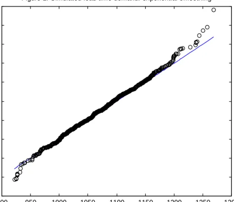
comparing the results of the bootstrap method for LLM(0) and LLM(1) was undertaken. First,

a sample was simulated from the LLM(1) with

m

=

100

,

s

=

0 05

.

and

n

=

30

. Maximum likelihood estimates were obtained for both models. These were then used obtain both

bootstrap samples of 1000 lead-time demands, the lead-time being

h

=

10

. Figure 1 shows the quantile-quantile plot of the samples. The plot is quite close to the 450 line reflecting the

similarity of the LLM(0) and LLM(1) lead-time demand distributions. This result is typical of

those obtained when the simulation conditions were varied.

Place Figure 1 about here

The parametric bootstrap approach ignores the effect of estimation error. An appropriate

adaptation of the simulation method described in Ord, Koehler and Snyder (1997) would

account for this source of error. It is anticipated that greater differences would then emerge

between the two models.

3. SIMPLE EXPONENTIAL SMOOTHING WITH DRIFT

3.1 L

OCAL

L

EVEL

M

ODELS WITH

D

RIFT

Intuitively, it makes sense that heteroscedasticity related to the magnitude of the fluctuations

in the mean, may be modest when the mean is locally constant. It is likely to have more of an

impact if there is a tendency for the series to increase or decrease over time. We therefore

introduce a growth rate b into (2.2) to give

y

t

m bt

e

j

e

j t t

= + +

+

= −

∑

α

1 1 . (3.1)

(14)

This can be written as

y

_t

= + +

m bt

u

_t where

u

_t

=

u

_t₋₁

−

θ

e

_t₋₁

+

e

_t. Differencing (3.1) yields

∆

y

_t

= −

b

θ

e

_t₋₁

+

e

_t so that the associated time series is ‘difference stationary’. Contrast this with the more common case where the trend is accompanied by first-order autocorrelated

disturbances governed by

u

_t

=

φ

u

_t₋₁

+

e

_t, the associated series now being ‘trend stationary’ provided that parameter

φ

satisfies the condition

φ <

1

.

The local level may be defined as

m

t

m bt

e

t j t

= + +

=

∑

α

1

. Then (3.1) may be written as

y

_t

=

m

_t₋₁

+ +

b

e

_t where

m

_t

=

m

_t₋₁

+ +

b

α

e

_t. This local level model with drift is the special case of the model underlying Holts trend corrected exponential smoothing where the growth

rate is restricted to a constant value. The generalisation to include heteroscedastic variation is

y

_t

=

1

m

_t₋1

+ +

b

6 1

m

_t₋1

+

b e

6

q _t (3.2)

where

m

_t

=

1

m

_t₋₁

+ +

b

6 1

α

m

_t₋₁

+

b e

6

q _t. (3.3)

It will be designated LLDM(q). Again

q

=

1

corresponds to the relative error case.

The local level, for any LLDM(q) can be written as

m

_t t

m

j

b

y

j t j t j j t

=

+

= = − −

∑

θ

α θ

1 0 1 .

The local level is still a discounted linear function of series values when the invertibility

condition

θ <

1

holds. In what follows, however, we continue to use the common restriction

0 ≤ ≤

α

1

.

(15)

Smoothing and estimation is quite similar to the case where there is no drift. For given values

of

m

,

b

and

. Using the principle of maximum likelihood, it can be argued

that

m b

,

and

α

should be chosen to minimise the generalised standard error

ω =

+

−

=

∏

s

m

_t

b

t n n q

|

₁

|

1 .

A simulation study similar to the first study described in section 2.3 was again conducted, but

now with a drift of

b

=

0 5

.

. Interestingly the simulated ratio

λ

now had a moderately larger average of 1.0015 and standard deviation of 0.0040. It seems that even with a drift term, the

LLDM(0) estimates are close enough for most practical purposes to use as approximations for

their LLDM(1) counterparts. Interestingly, the optimal generalised standard error

ω

1 *

was

now greater than

ω

*₀ about 80 percent of the 1000 replications. Furthermore, the gap between

ω

0 *

and

ω

₁* now exceeded one percent in 67 percent of the replications. The differences between LLDM(0) and LLDM(1) when there is drift can be quite marked.

3.3 L

EAD

T

IME

D

EMAND

D

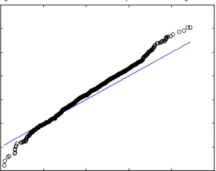
ISTRIBUTION

It is possible to obtain formulae for the mean and standard deviation of the lead-time

demand distributions. It is simplest, however, to undertake a parametric bootstrap of

the lead-time distribution. Figure 2 shows the quantile-quantile plot obtained when the

simulation was conducted under essentially the same conditions as those depicted in

section 2.4. The only difference is that now a drift of b

=

0 5

. is assumed. The

quantile-quantile plot of simulated lead-time demands is now steeper than the 45

0

line.

This indicates that the lead-time demand distribution for LLDM(1) is more spread

(16)

than that for LLDM(0). It suggests that larger safety stocks may be required if level

dependent errors are present and that a pronounced drift is observed in demand.

Place Figure 2 about here

4. Trend Corrected Exponential Smoothing

Another possible model is

y

_t

m bt

e

_j

e

j t j t j i i t

= + +

+

= − = = −

∑

α

1

α

1 1 2 1 1 1 . It may be written as

y

_t

>

2

, the parameters being related by the equations

θ

₁

= −

2 α α

₁

−

₂ and

θ

₂

=

α

₁

−

1

. It is a trend line with a particular form of autocorrelated disturbances. A local level may be defined as

m

t

m bt

e

j

e

j t j j i i t

= + +

+

= = =

∑

α

1

α

1 2 1 1 . Then

y

t

m

t

b

e

j

e

j t t

=

₋

+ +

+

= −

∑

1 2 1 1

α

. If, in addition, a

local growth rate is defined as

b

t

b

e

j j t

= +

=

∑

α

2 1

, then the model may be written is state space

form as

y

_t

=

m

_t₋₁

+

b

_t₋₁

+

e

_t where

m

_t

=

m

_t₋₁

+

b

_t₋₁

+

α

₁

e

_t and

b

_t

=

b

_t₋₁

+

α

₂

e

_t. Unlike LLDM(0), the growth rate is now allowed to change over time. This is the so-called local

trend model.

A generalisation to accommodate heteroscedastic variation is

y

_t

=

m

_t₋1

+

b

_t₋1

+

1

m

_t₋1

+

b

_t₋1

6

q

e

_t (4.1)

₋1

+

α

2

1

₋1

+

₋1

6

_(4.3)

It will be designated LTM(q). Again

q

=

1

corresponds to the relative error case.

Assuming that m, b,

α

1 and

α

2 have been assigned trial values, the information available at

the end of typical period t is

I

t

=

;

y

1

,

!

,

y m b

t

, , ,

α α

1

,

2

@

. Let

m

0

_t

=

1 6

b I

_t

|

_t for

t

7

(4.4)

b

_t

=

b

_t₋1

+

α

2

y

_t

−

m

_t₋1

−

b

_t₋1

7

, (4.5)

These recurrence relationships are obtained by eliminating the

e

t from the LTM(q) equations.

They correspond to the error correction form of Holts trend corrected exponential smoothing

(Gardner, 198*). Thus this traditional method is applicable under much broader conditions

than those traditionally stated in the literature. It applies when the variation depends on the

underlying level.

Maximum likelihood estimates of m, b,

α

₁ and

α

₂ can be obtained by minimising the

generalised standard error

ω =

+

− −

=

∏

s

m

_t

b

_t t n n q

|

1 1

|

1

. The standard deviation

s

is still

calculated from the formula

s

e

t

n

i n 2 2 1

=

∑

but now the errors are obtained from trend

corrected exponential smoothing using the formula e

_t

=

2

y

_t

−

m

_t₋₁

−

b

_t₋₁

7 2

m

_t₋₁

+

b

_t₋₁

7

q. LTM(q) reduces to LLDM(q) when

α

2

=

0

. Both models have similar properties so the

(18)

conclusions reached with the simulations for LLDM(q) also apply to LTM(q).

5. Seasonal

Effects

LTM(0) can be augmented by a seasonal cycle of length p if required. Let

c

t denote the

seasonal effect associated with typical period t. The resulting model, when the seasonal

effects are additive, is

y

_t

=

m

_t₋₁

+

b

_t₋₁

+

c

_{t p}₋

+

e

_t where

m

_t

t. It is easily seen that this model underpins the additive

version of Holts seasonal exponential smoothing. Its multiplicative counterpart is

y

t

=

1

m

t−1

61

1 +

α

1

e

t

6

c

t

=

c

t p−

1

1 +

α

3

e

t

6

. If the errors are substituted out of these

equations and the appropriate conditioning on past information is undertaken, the equations

for Winters method of exponential smoothing is obtained (Winters, 1960). The details are

covered in Ord, Koehler and Snyder (1997).

To reduce the number of parameters it is often better to use a Fourier representation of

seasonal cycles (Brown, 196X). Winters method would not be practical if applied to say

weekly demand data. One possibility is a linear local level model with drift and seasonal

cycle LLDSM(0)

y

m

b

c

e

m

b

ae

c

t

t t t p t t t t t j j j j j r

=

+ +

+

=

+ +

=

+

− − − =

∑

1 1 1

α

sin

3 8

ω

γ

cos

3 8

ω

4

9

where the

ω

_j are the frequencies and the

α

_j and

β

_j are coefficients. Note that

r

≤

1 6

p

+

1 2

. Usually r is much smaller than

1 6

p

+

1 2

. Otherwise there would be no advantage in using Fourier representations. In this model the seasonal cycle is deterministic.

(19)

the seasonal cycle follows a random walk, something that is difficult to believe. Another

possible generalisation involves local growth rates as found in the local trend model.

A nonlinear heteroscedastic generalisation of this model is:

y

m

b

c

e

m

b

ae

c

t

t t t p t t t t t j j j j j r

=

+

=

+

=

+

− − − =

∑

1 1 1

1

63 81 6

1 61 6

3 8

4

α

sin

ω

γ

cos

ω

9

.

The seasonal and irregular components increase with the trend. This model will be designated

LLDSM(1).

Again the generalised standard error may be used as the estimation criterion. It is

ω =

−

₋

− −

₋ =

∑

y

_t

m

_t

b

c

_{t p}

n

t n 1 2 1

3

8

and

ω =

−

+

− − − −

+

= = − −

∑

y

t

_m

m

t

_b

b

_c

c

t p

n

∏

m

b

c

t t p t n t t p t n n 1 1 2 1 1 1

1

63

8

1

63

8

1

63

8

for LLDSM(0) and LLDSM(1) respectively.

A simulation study similar to the one described in section 3.3 was undertaken to determine the

differences in the estimates for the linear and nonlinear cases. The series for the simulation

were generated from the nonlinear model with

c

_t

=

0 5

. sin

1

2 π

t

52

6

. This corresponds to a pronounced seasonal cycle in the time series but the size of the amplitude of the cycle is quite

plausible in practice. On average the generalised standard error turned out to be about 20

percent higher for the estimates based on the wrong LLDSM(0). Using the generalised

(20)

time. Thus, for the first time, we have detected a major difference between the homoscedastic

and heteroscedastic models. The implications of this will be explored in greater depth using

criteria from inventory control.

INVENTORY CONTROL

In this section we attempt to gauge the impact of differences arising from the linear and

nonlinear seasonal models in the context of an inventory problem. The focus will be on an

order level system with periodic reviews and the backlogging of excess demand.

The state of an order level system at any point of time is represented by the stock position, a

quantity governed by the formula StockPosition = Stock – Backlog + OnOrder. The order

level represents the appropriate level for the stock position following the placement of a new

replenishment order. It is assumed that such orders are placed at the start of each review

period.

The size of the order level determines the service given to customers. It is assumed that

service is summarised by the fill-rate (customer service level), a statistic that measures the

proportion of demand satisfied without delays caused by shortages. It is further assumed that

managers specify a target value for the fill-rate, the problem then being to choose the order

level to meet this target.

A theory for the determination of order levels using the fill-rate (customer service level)

statistic appears to have been first proposed by Brown (19??). The theory involves the use of

exponential smoothing in combination with what Brown refers to as a ‘partial expectation’.

The approach was a major breakthrough in its day and its influence may still be found in

modern inventory control software. It has, however, two weaknesses that can nowadays be

circumvented with the common availability of powerful computers.

(21)

lead-time demand.

b) It relied on an approximation for the fill-rate that was a necessary convenience when

calculations were done manually, but which is known to be inaccurate when review

periods are short in length – see below for details.

The theory of this paper provides an opportunity to circumvent the heuristics for measuring

variability while using the exact formula for the customer service level. We now outline a

parametric bootstrap approach that would have been impractical until recent times. It is based

on the assumption that an order placed at time n is delivered at time

n

+

h

and that the problem is therefore to use such an order to influence the performance of the inventory system

in the period

1

n

+

h n

,

+ +

h

1

6

. The fill-rate in this period is defined as

β = −

1 E x

3

_{n h}_{+ +}₁_|_n

8 3

E y

_{n h}_{+ +}₁_|_n

8

where

x

_{n h}_{+ +}_1|_n is the excess demand in period n+h+1 and

y

_{n h}_{+ +}1|_n is the demand in period n+h+1 given the information set In. Since

x

_{n h}_{+ +}1|_n

≤

y

_{n h}_{+ +}1|_n

the fill-rate always lies in the interval [0, 1]. This measure of service should not be confused

with the tail of the lead time demand distribution commonly used in some approaches to

inventory control (Buffa, 19??).

Demand in period n+h+1 may be easily simulated from the model underlying the forecast

method using parameter estimates in place of the unknown parameters. Given a particular

order level S, the corresponding excess demand in the same period can also be calculated with

x

_{n h}_{+ +}₁_|_n

=

4

y

₁

_n_{+ + +}₁_:_{n h} ₁

₆

_|_n

−

S

9 4

+

−

y

₁

_n_{+ +}₁_:_{n h n}

₆

_|

−

S

9

+. Each RHS term, being the excess of lead-time demand over total supply, is a backlog. They correspond to the closing and opening

backlog in period n+h+1 given the information In. Being the increase in the backlog, the RHS

corresponds to the excess demand in period n+h+1. It is possible to follow Brown (1959) and

assume that the opening backlog is small enough to be ignored. The second term on the RHS

(22)

periods are relatively short, a delivery may be insufficient to completely eliminate an existing

backlog. It is better not to make this approximation.

A bootstrap involving R replications may be used to estimate the fill rate. Denoting the rth

replication of excess demand and demand by

x

_{n h}

1 6

r_{+ +}_1|_n and

y

_{n h}

1 6

r_{+ +}_1|_n respectively, a bootstrap

estimate of the fill-rate is

β = −

_{+ +}_| _|

= = + +

∑

1

₁ 1 1 1

x

_{n h}r _n

y

r R n h n r r R

1 6

_.

The fill-rate depends on the order level S, a relationship that may be represented by the

1 6

S

as an approximation for

β

1 6

S

, the problem can be revamped to one of finding the solution

S

_of

the equation

β

1 6

S

=

β

.

The parametric bootstrap procedure consists of the following steps:

a) Simulate from the appropriate exponential smoothing demand model the

y

_{n j n}

1 6

r₊ _| for

j

=

1

to

h

+

1

,

r

=

1

to R.

b) Use a binary search procedure to solve the implicit function equation

β

1 6

S

=

β

for

S

.

Note that

β

1 6

S

is evaluated at step (b) for each trial value of S using the demands from step (a). There is no need to regenerate the demands for each function evaluation.

This bootstrap procedure is easily implemented on modern computers. But it is likely to yield

values for the order level slightly below those actually required because the parametric

(23)

to largely overcome this problem using a more complex prediction methodology from Ord,

Koehler and Snyder (1997). This option is not pursued here.

The fill rate is an appropriate criterion for evaluating whether there are significant gains from

using a relative error rather than an additive error approach to forecasting when it is known

that demands are generated by a relative error model. Any differences that might occur can be

gauged from a simulation study. Let LLDSM(

q,

θ

) denote the local level with drift and seasonal cycle model with parameter vector

θ

. Furthermore, let

θ

q denote the maximum

likelihood estimate of the parameter vector

θ

from LLDSM(q). The steps in each replication of the simulation are:

) and evaluate the fill rates achieved with

S

₀ and

S

ignoring the estimation error in the parametric bootstrap or any bias in the forecast procedure.

In the simulation study it was assumed that:

a) The stock position is reviewed at the beginning of each week.

b) Orders are delivered after a delay of 9 weeks. Thus the aim is to control inventories in

the week following the delivery, namely week 114 (2*52+9+1).

c) Deliveries occur at the start of a week, immediately following the review.

d) Weekly demand is governed by the LLDSM(1) with

m

=

100

,

b

=

0 1

.

,

c

_t

=

0 5

. sin

1

2 π

t

52

6

,

a

=

0 5

.

and

s

=

0 05

.

. The growth rate, in annual terms, is 5.2 (ie 0.1 * 52 weeks). This, relative to the initial level, is a little over 5 percent per

annum.

e) Weekly demand data for two years is available for forecasting purposes so that the

current review occurs at the beginning of period 105 (ie 2*52+1).

f) The target fill-rate is

β =

95%

.

A number of simulation experiments were conducted under a variety of conditions. Each

simulation experiment involved 200 replications. At each replication the bootstrap method for

finding the order level itself involved 1000 replications. The results are summarised in Table

2. The benchmark case represents a situation that we think may be fairly typical in the

inventory control context. The other cases were obtained by varying one factor at a time from

its benchmark value.

(25)

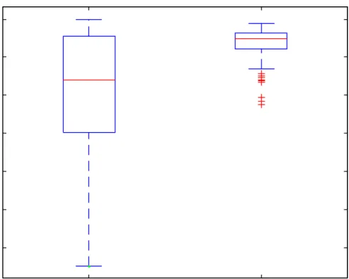
The following observations can be made.

a) The means are generally below the medians. The distributions of the simulated

fill-rate must possess a left skew. This is exemplified by the distribution in Figure 3 for

the benchmark case.

b) The medians obtained with the bootstrap method from LLDM(1) are usually about

one percent below the target fill-rate of 95 percent. This gap is probably due to the

fact that the bootstrap method ignores the effect of estimation error. Given the size of

this gap, refinements geared to eliminating this problem appear to be unwarranted.

c) The median fill-rates associated with LLDM(0) are little lower again. There appear to

be some gains from using the relative error approach when the data generating

process involves relative errors.

d) The gains from using the bootstrap method with LLDM(1) instead of LLDM(0)

increase with higher growth rates. The changes in the underlying level are larger and

the fluctuations of the irregular component increase as a consequence. Nevertheless,

the growth rate has to reach unrealistic levels before the differences become

pronounced.

e) Variations in most factors have little impact on the median fill-rate for the LLDM(1)

bootstrap method.

4. CONCLUSIONS

In this paper we have proposed a generalisation of the additive local level model or its

equivalent, the ARIMA(0,1,1) model, to incorporate a general form of conditional

(26)

form, remains the valid updating relationship under this more general class of models. The

only change required is in the form of the criterion function used for selecting the estimates. A

simulation indicated that the maximum likelihood estimates obtained with simple exponential

smoothing under a level dependent form of heteroscedasticity are almost identical to those for

the homoscedastic case. Since the homoscedastic case is inherently easier to estimate than its

multiplicative counterpart we recommend the use of the former for estimation purposes.

The issue of heteroscedasticity becomes more critical in the prediction context. Analytical

formulae become unreliable for the multiplicative case. We therefore recommend a two-stage

procedure:

a) estimate

m

,

a

and

s

using the additive model

b) use the estimates from the previous step in conjunction with the multiplicative model to

simulate the prediction intervals.

Appendix

This appendix contains the derivation of the formulae for the mean and variance of the linear

and multiplicative local trend/seasonal models. To simplify notation the origin for forecasting,

designated period n in the body of the paper, will be relabelled period 0. The prediction

horizon is designated by h. Thus the random h-vector

y

=

y

₁

y

₂

"

y

_h

′

designates h unknown future values of the time series. Furthermore,

A

0 and

b

0 denote the local level and

local rate at the start of the prediction origin. They no longer represent the seed values for

these quantities in the period prior to the sample. These quantities are known exactly. The

vector

γ =

c

_{− +}_r ₁

c

_{− +}_r ₂

"

c

₀

′

of seasonal factors required for forecasting is also known exactly. The formulae to be derived in this appendix are therefore based on the assumption

(27)

The derivations rely extensively on a matrix B called the ‘backward shift’ matrix. It is the

matrix counterpart of the backward shift operator used so extensively in Box and Jenkins

(19XX). The notation employed, together with explanations, is shown in the following Table.

To simplify matters it is assumed that h is an exact multiple of the seasonal lag r. Let

m

=

h r

. It is the length of the forecast horizon measured in years.

h

′

τ

1 6

2

the series h-vector

1 3 6 10

"

h h

1 6

+

1 2

B

the backward shift matrix where

b

ii−1

=

1

for i=1,!,n and

b

ij

=

0

otherwise.

eg

0

1

0

1

0

1 2 3 1 2

!

"

_$

##

_#

_!

"

_$

##

_#

=

!

"

_$

##

_#

x

B

r the backward shift matrix of lag r where

b

ii r−

=

1

for i= +r 1,!,n and

b

ij

=

0

otherwise.

eg. if

B

=

!

"

$

##

0

1

0

1

0

1

0

then

B

2

0

1

0

1

0

0 =

!

"

$

##

and

0

1

0

1

0

1 2 3 4 1 2

!

"

$

##

!

"

$

##

=

!

"

$

##

x

.

(28)

S partial sum matrix being a unit lower triangular matrix with all elements below the diagonal equal to 1. eg.

S

=

!

1 0 0

"

_$

##

_#

1 1 0

1 1

1

so that

1 0

0 1 1

1

1 2 3 1 1 2 1 2 3

!

"

_$

##

_#

_!

"

_$

##

_#

=

+

+ +

!

"

_$

##

_#

x

. Note that

S

= −

1 6

I

B

−1

= + +

I

B

2

+ +

"

B

n−1

S

1 6

r defined by

S

1 6

r

= −

2 7

I

B

r −

= +

I

B

r

+

B

r

+ +

B

mr 1 ₂

"

Ξ

_{Ξ =}

S

= −

1 6

I

B

−1

I

+

BS

= +

I

SB

=

S

ξ =

1 S1

= τ

ξ +

B1

=

1

1 +

B

τ τ

=

_S

1 6

r

_{Ξ =}

µ µ

₁

+

₂ and variance matrix

AA'

where

µ

₁

=

1 A

₀

+

τ

b

₀,

µ

₂

=

Z

γ

and