Diabetes Forecasting Using Supervised Learning Techniques

(1)

Diabetes Forecasting Using Supervised Learning Techniques

Salim Amour Diwani1, Anael Sam2

1

Computational and Communication Science and Engineering, Nelson Mandela African Institution of Science and Technology Arusha, P.O.BOX 447, Tanzania

[email protected]

2

Computational and Communication Science and Engineering, Nelson Mandela African Institution of Science and Technology Arusha, P.O.BOX 447, Tanzania

[email protected]

Abstract

Diabetes Mellitus is one of the most serious health challenges affecting children, adolescents and young adults in both developing and developed countries. To predict hidden patterns of diseases diagnostic in the healthcare sector, nowadays we use various data mining techniques. In this paper, we have applied supervised machine learning techniques like Naive Bayes and J48 decision tree to identify diabetic patients. We evaluated the proposed methods on Pima Indian diabetes data sets, which is a data mining data sets from UCI machine learning laboratory. It has been observed through analysis of the experimental results that Naive Bayes performs better than the decision tree method J48.

Keywords: Data Mining, Naive Bayes, J48, Neural Network,

Diabetes, MRBF, RBF, CVD, CHD, ROC, SVM, KNN.

1. Introduction

Diabetes Mellitus is one of the most widespread chronic diseases of childhood, affecting children, adolescents and young adults. Diabetes is a condition in which a human body is unable to produce the required amount of insulin needed to regulate the amount of sugar in the body [1]. This Phenomenon leads to various diseases including cardiovascular diseases, blindness, kidney failure, and lower limb amputation. Maintaining blood glucose levels, blood pressure and cholesterol at normal range can help delay or prevent diabetes complications arising due to diabetes. Therefore diabetic patients need regular monitoring. In 2013, 382 million people worldwide were reported with diabetes: - 24 million in South and Central America, 37 million in North America and the Caribbean, 56 million in Europe, 35 million in the Middle east and North Africa, 20 million in Africa and 138 million in Western Pacific and it is predicted that 592 million people worldwide will live with diabetes in 2035 [2].

As the prevalence of diabetes continues to grow worldwide, related diseases like morbidity and mortality

are emerging as a major health care problem. Patients with diabetes are at increased risk of developing and dying from cardiovascular diseases (CVD). People with diabetes have been shown to have twice the risk of CVD as the general population [2]. Moreover, Coronary Heart Disease (CHD) is the leading cause of death among adults with diabetes [3]. Diabetes disease diagnosis and interpretation of data is an important classification problem [4]. A classifier is required to be designed in an efficient way, cost effective and accurate manner. A medical diagnosis is a classification process where a physician has to analyze a lot of factors before diagnosing a patient with diabetes, which is generally, seems to be a difficult problem. In the past, various statistical methods have been used for modeling in the area of diseases diagnosis. However most of the methods requires prior assumptions and are less capable of dealing with massive and complicated non-linear and dependent data [5]. Data mining has been proven to be more powerful and effective approach which provides process for discovering useful patterns from large data sets [6]. Recently, many methods and algorithms including Neural networks (NNs), Decision Trees (DTs), Fuzzy Logic Systems, Naive Bayes, SVM, Categorization, Logistic Regression are proposed by different researchers to mine biomedical datasets for identification of hidden patterns embedded within them [7,8,9]. These algorithms minimize time for the medical treatment, providing safe health care treatment and providing various healthcare treatments based on patients' needs, symptoms and preferences. A brief description of the general symptoms of diabetes is given in Table 1.

(2)

Table 1: General Symptoms of Diabetes [10] Symptoms Name Description

Excessive Thirst and Increased Urination

When you have diabetes, excess sugar (glucose) builds up in your blood. This triggers more frequent urination, which may leave you dehydrated. As you drink more fluids to quench your thirst, you will urinate even more

Fatigue You may feel fatigued. Many factors can contribute to this. They include dehydration from increased urination and your body's inability to function properly, since it's less able to use sugar for energy needs.

Weight loss Weight fluctuations also fall under the umbrella of possible diabetes signs and symptoms. When you lose sugar through frequent urination, you also lose calories.

Red, swollen, tender gums

Diabetes may weaken your ability to fight germs, which increases the risk of infection in your gums and in the bones that hold your teeth in place. Your gums may pull away from your teeth, your teeth may become loose, or you may develop sores or pockets of pus in your gums.

A tingling sensation or numbness in the hands or feet

Excess sugar in your blood can lead to nerve damage. You may notice tingling and loss of sensation in your hands and feet, as well as burning pain in your arms, hands, legs and feet.

Blurred vision Diabetes symptoms sometimes involve your vision. High levels of blood sugar pull fluid from your tissues, including the lenses of your eyes. This affects your ability to focus.

Frequent infections and Slow-healing wounds

Doctors and people with diabetes have observed that infections seem more common if you have diabetes. High levels of blood sugar impair your body's natural healing process and your ability to fight infections.

Tingling hands and feet

Excess sugar in your blood can lead to nerve damage. You may notice tingling and loss of sensation in your hands and feet, as well as burning pain in your arms, hands, legs and feet.

1.1 Data Mining

Data mining is an emerging technology with the development of artificial intelligence and database techniques which is used in different business organizations to improve the efficiency and effectiveness of a business process [11]. Data Mining is an interdisciplinary field that combines artificial intelligence, computer science, machine learning, database management, data visualization, mathematics algorithms and statistics [12]. Data Mining is a variety of techniques such as neural network, decision trees or standard statistical techniques to identify nuggets of information or decision making knowledge in bodies of data, and extracting these in such a way that they can be put to use in areas such as decision support, prediction, forecasting and estimation [13]. This techniques uses classification algorithms such as Naive Bayes, Logistic Regression, J48 Decision Tree, Cluster Analysis, Simple k-means and other statistics methods to find out, from large un-organized data

set, useful information for business operation[14]. While the historical data of most enterprises are millions and millions of data which are very difficult to analyze, it has becomes important to extract useful information from large amount of data [15].

2. Related Works

Kumari and Chitra [16] used support vector machine (SVM) a machine learning method a supervised machine learning method, as a classifier for diagnosing diabetes. Their experimental results showed that SVM can be successfully used for diagnosing diabetes diseases. The system was developed by designing the experiments using MATLAB 2010a. The data sets were stored in excel documents and read direct from MATLAB. The diagnostic performance of the developed model was evaluated using receiver operating characteristics (ROC) curve. In the ROC curve the true positive rate is plotted as function of the false positive rate for different cut off points. Each point in the ROC curve represents a sensitivity pair corresponding to a particular decision threshold. To evaluate the robustness of the SVM model, the 10 fold cross validation for training sets was used and the process was repeated ten times for test sets which assess the performance of the model.

Magudeeswaran and Suganyadevi [17] used modified radial basis functional neural networks (MRBF), a supervised machine learning method, as a classifier to predict diabetes for patients. The technique used the blood glucose level for diabetes patients for prediction. The proposed approach was evaluated by the Pima Indian diabetes data sets and observed from the experimental results that the MRBF obtained better results than the existing radial basis functional (RBF) methods and other neural network. The results were compared with other data mining techniques such as Nearest Neighbor, K-nearest neighbor, K-nearest neighbor with backward sequential selection of feature and multiple feature subsets and the proposed model proved to be better than other models and the algorithms with which was compared. Therefore, MRBF neural network approach provides better and fastest results compared to the existing RBF neural network for predicting diabetes patients. The MBRF is envisioned by using GA for optimally deciding the number of neurons in single hidden layer architecture.

Vijayalakshmi and Thilagavathi [18] used b-coloring technique in clustering analysis, a supervised machine learning method as an approach to predict diabetes diseases for Pima Indian diabetes data sets. The proposed technique presents a real representation of clusters by dominant objects that assures inter cluster disparity in a

(3)

partitioning and used to evaluate the quality of cluster. The proposed algorithms were k-nearest neighbour (KNN) classification and k-means clustering and the results showed that the clustering based on graph coloring perform better than the other clustering algorithms in terms of accuracy and parity.

3. Methodology

The Pima Indian diabetes database was introduced by Vincent Sigillito in 1988 as the owner of the database [19]. Pima Indian is a collection of 768 samples or instances from a population living near Phoenix Arizona which investigated whether a person shows a sign of diabetes or not according to the World Health Organization (WHO). In his paper Vincent used ADAP algorithm which is an adaptive learning routine that generates and executes digital analogs of perception like devices.

Figure 1: Methodology Interface

3.1 Experiments

In order to train the classifier of diabetes, 768 samples are used for training and testing. For creating diabetes status predictive model J48 and Naive Bayes algorithm are used. To evaluate the performance of the model; 10 cross validation is used due to its relative low bias and variations. This means the data are randomly partitioned equally into ten parts. The learning scheme is trained ten times using nine-tenths of the total data and the remaining is used for testing. Therefore the learning procedure is executed a total of 10 times on different training and testing sets. In the experiment 9 selected attributes including preg, plas, pres, skin, insu, mass, pedi, age and class are used. The experiment is done using WEKA data mining tool version 3.6.11. The tool takes the data in arff format in a single table, before that the prepared data in excel format is changed to CSV

format.

Figure 2: Arff File Format

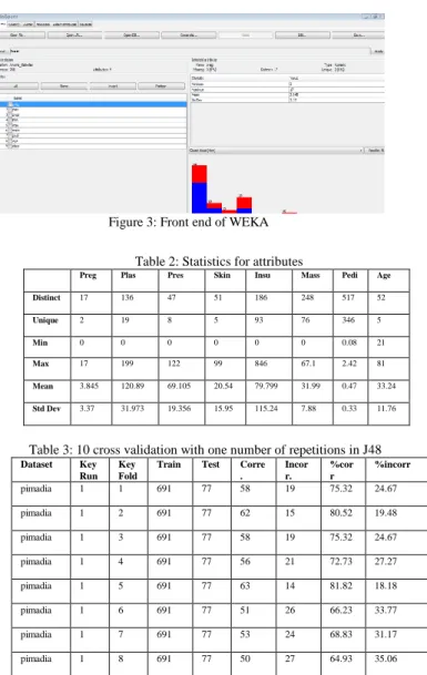
As shown in figure 2 above, the arff file format consists of name of the relation, list of attributes with their corresponding values and the client data. In order to build a model this arff file is given to the classifiers. The front end of this file is shown in figure 3 below:

Figure 3: Front end of WEKA Table 2: Statistics for attributes

Preg Plas Pres Skin Insu Mass Pedi Age

Distinct 17 136 47 51 186 248 517 52 Unique 2 19 8 5 93 76 346 5 Min 0 0 0 0 0 0 0.08 21 Max 17 199 122 99 846 67.1 2.42 81 Mean 3.845 120.89 69.105 20.54 79.799 31.99 0.47 33.24 Std Dev 3.37 31.973 19.356 15.95 115.24 7.88 0.33 11.76

Table 3: 10 cross validation with one number of repetitions in J48

Dataset Key Run

Key Fold

Train Test Corre . Incor r. %cor r %incorr pimadia 1 1 691 77 58 19 75.32 24.67 pimadia 1 2 691 77 62 15 80.52 19.48 pimadia 1 3 691 77 58 19 75.32 24.67 pimadia 1 4 691 77 56 21 72.73 27.27 pimadia 1 5 691 77 63 14 81.82 18.18 pimadia 1 6 691 77 51 26 66.23 33.77 pimadia 1 7 691 77 53 24 68.83 31.17 pimadia 1 8 691 77 50 27 64.93 35.06

(4)

Table 4: 10 cross validation with one repetition in Naive Bayes Dataset KeyRun KeyFold Train Test Corr Incorr %corr %incorr pimadiab 1 1 691 77 63 14 81.82 18.18 pimadiab 1 2 691 77 64 13 83.12 16.88 pimadiab 1 3 691 77 60 17 77.92 22.077 pimadiab 1 4 691 77 63 14 81.82 18.18 pimadiab 1 5 691 77 56 21 72.73 27.27 pimadiab 1 6 691 77 57 20 74.03 25.97 pimadiab 1 7 691 77 54 23 70.13 29.87 pimadiab 1 8 691 77 51 26 66.23 33.77 pimadiab 1 9 692 76 58 18 76.32 23.68 pimadiab 1 10 692 76 60 16 78.95 21.05

3.2 Model Building

3.2.1 Histogram

By comparing the histograms for all of the input attributes, we began to get a sense of how the 8 input attributes vary with different species. For example preg sample appears to have 17 distinct values and 2 unique values with standard deviation of 3.845 and plasma appears to have 136 distinct values and 19 unique values. Therefore these are the types of patterns that data mining algorithms use to perform classification and other functions. A re-examination of the histograms in Figure 4 below shows that how difficult in making decision, therefore decision tree is the best option in making right decision.

Figure 4: Histogram

4. Data Mining Techniques

To. build the predictive model of J48 and Naive Bayes algorithms are trained and evaluated. For the purpose of this paper it has been attempted to find whether Naive Bayes classifier performs better than J48 by identifying the important parameters of the algorithms. The J48 decision tree classifiers follows an algorithm in order to classify a new item, it first needs to create a decision tree based on the attributes values of the available training data.

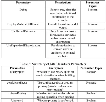
Table 5: Summary of Naive Bayes Classifiers Parameters

Parameters Descriptions Parameter

Types Debug If set to true, classifier

may output additional information to the

console

Boolean

DisplayModelInOldFormat Use old format for model output

Boolean

UseKernelEstimator Use a kernel estimator for numeric attributes rather than a normal

distribution

Boolean

UseSupervisedDiscretization Use discretization to convert numeric attributes to nominal

attributes

Boolean

Table 6: Summary of J48 Classifiers Parameters

Parameters Descriptions Parameter Types

binarySplits Whether to use binary splits on nominal attributes when building

the trees.

Boolean

confidenceFactor The confidence factor used for pruning (smaller values incur

more pruning).

Numeric

subtreeRaising Whether to consider the subtree raising operation when pruning

Boolean

Unpruned Whether pruning is performed. Boolean

So whenever it encounters a set of items (training set) it identifies the attribute that discriminate the various instances most clearly. As shown in the tables above, J48 has smaller value of confidence factor which help to enforce more pruning. The default confidence factor is 0.25. Confidence factor works only when the unpruned parameter is set to False. The confidence factor can be increased or decreased and the number of instances can also be increased or decreased. On the other hand Naive Bayes follows the probability distribution over all classes and the evidence can be splits into parts that are independent. Also the outputs of several classifiers can be combined, for example by multiplying the probabilities that all classifiers predict for a given class and with each training example, the prior and likely hood can be updated dynamically: flexible and robust to errors.

Refer to the Figure 5 and Figure 6 which shows the accuracy of the two models Naive Bayes and J48 (76.3 and 73.8) respectively. Now if you compare the Kappa Statistics of Naive Bayes and J48, the Naive Bayes which is 0.46 looks much stronger than compared to J48 which is 0.41. This can be analyzed using Confusion Matrix at the bottom of the classifier output window.

(5)

Figure 5: Classifier Accuracy for Naive Bayes

Therefore, there are 422 true positive, 104 false positive, 78 false negative and 164 true negative for Naive Bayes and 407 true positive, 108 false positive, 93 false negative and 160 true negative for J48. Hence, the model for Naive Bayes exhibit an excellent value of ROC curve which is 0.8 depicting the active area. This shows that the Naive Bayes model could be very advantageously be used for predicting patients with diabetes compared with J48. This can be shown clearly by analyzing ROC and cost benefits plots.

Figure 6: Classifier Accuracy for J48

A naive Bayes technique provides probabilistic outputs. This means that Naive Bayes model can assess the value of the probability varying from 0 to 1 and that a given model can be predicted as active by moving the threshold from 0-1.

4.1 Naive Bayes

The Naïve Bayes classifier algorithm works on a simple, but comparatively intuitive concept. Also, in some cases it is also seen that Naïve Bayes outperforms many other comparatively complex algorithms. It makes use of the variables contained in the data sample, by observing them individually, independent of each other.The Naïve Bayes

classifier is based on the Bayes rule of conditional probability. It makes use of all the attributes contained in the data, and analyses them individually as though they are equally important and independent of each other.

Pr [ H│E ] = Pr[E│H] Pr[H]

Pr [E]

Class Instance

Table 7: Naive Bayes Classifier model (full training set) Attribute Class tested negative

(0.65)

Class tested positive (0.35) Preg Mean 3.4234 4.9795 Std.dev 3.0166 3.6827 Weight sum 500 268 Precision 1.0625 1.0625 Plas Mean 109.9541 141.2581 Std.dev 26.1114 31.8728 Weight sum 500 268 Precision 1.4741 1.4741 Pres Mean 68.1397 70.718 Std.dev 17.9834 21.4094 Weight sum 500 268 Precision 2.6522 2.6522 Skin Mean 19.8356 22.2824 Std.dev 14.8974 17.6992 Weight sum 500 268 Precision 1.98 1.98 Insu Mean 68.8507 100.2812 Std.dev 98.828 138.4883 Weight sum 500 268 Precision 4.573 4.573 Mass Mean 30.3009 35.1475 Std.dev 7.6833 7.2537 Weight sum 500 268 Precision 0.2717 0.2717 Pedi Mean 0.4297 0.5504 Std.dev 0.2986 0.3715 Weight sum 500 268 Precision 0.0045 0.0045 Age Mean 31.2494 37.0808 Std.dev 11.6059 10.9146 Weight sum 500 268 Precision 1.1765 1.1765

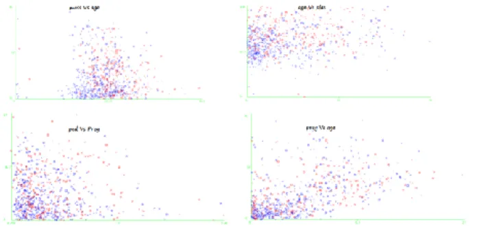
Refer to Figure 7 which shows visualized classifier assignment. Blue colors represents tested negative and red color represent tested positive. The classifier for body mass and age, 135 instances classifies as negative but 3 of them were incorrectly classified. Classifier errors for age and plas, 202 instances classified as TB tested negative and 22 of them were incorrectly classified. The classifier

(6)

Figure 7: Classifier Assignment

errors for pedi and pregnancy, 118 instances classified as TB tested negative and 34 were incorrectly classified. The classifier error for pregnancy and age, 4 instances were classified as positive and no any sample were misclassified.

Figure 8: ROC Curve

Refer to figure 8 which shows ROC curve for diabetes mellitus. The x-axis represents false positive rate and y-axis represents true positive rate. The color depicts the value of the curve. The colder region closer to the blue color corresponds to the lower threshold value. In the graph the value of the true positive rate exceed the false positive rate which indicated by angle closer to 90 degrees, hence the classification model for diabetes is predicted as active. In order to find the optimal value of the ROC curve for diabetes, we need to perform cost benefit analysis as shown in Figure 9. The left curve is the threshold curve or lift curve for diabetes, which look somehow similar with ROC curve but they're not. The threshold curve on the x-axis represents the sample size and the y-x-axis represents true positive rate. The threshold curve for diabetes have the confusion matrix which is shown in Figure 10, if you pay close attention to the confusion matrix of the current value of the threshold sharply differs from the previously obtained one. In particular, the classification accuracy 65.1% is considerably lower than the previous value 76.3021%, the number of the false negative greatly increased from 78 to 500 where as the number of true negative also increased from 164 to 268.

Figure 9: Cost Benefit Analysis Curve

Figure 10: Confusion Matrix

Refer to Figure 11 which shows the cost matrix for diabetes mellitus. The four entries indicate the cost one should pay for decision taken on the base of classification model. The cost values are expressed in abstract units, however it can be considered in a money scale for example in Tanzanian Shillings. The left bottom cell of the cost matrix defines the cost of false positive and its default value is 1 unit. This is the price which one should pay in order to synthesize and wrongly tested the predicted model as active. The right top cell of the cost matrix defines the cost of false negative and its default value is 1. This corresponds to the mean price one should pay for throwing away a useful part of the model and losing profit because of the wrong prediction taken by the classification model. It is also taken by default one should not pay price for correct decisions taken using classification model. The overall cost corresponding to the current value of the threshold is 500.

Figure 11: Cost Matrix

Figure 12 shows the Margin curve which generates points illustrating the prediction margin for diabetes mellitus. The margin is defined as the difference between the probability predicted for the actual class and the highest probability predicted for the other classes.

(7)

Figure 12: Margin Curve

4.2 Decision Tree (J48)

Decision tree j48 is the implementation of algorithm ID3 (Iterative Dichotormiser 3) developed by the WEKA project team. It is a decision tree classifier which decides a target value of a new sample based on various attributes values of the available data. The internal node of the decision tree denotes the different attributes; the branches between the nodes tell us the possible values that these attributes can have in the observed samples, while the terminal nodes tell us the final node of the dependent variable. Figure 13, shows that decision tree has 20 leaves and total size of the tree is 39 elements, which tells us how the decision was made using the tree. For example, if plas is less or equal to 127 and mass is less than or equal to 26.4 then the patient who tested negative were 135, but 3 of them were classified incorrectly as tested positive.

Figure 14: PRISM J48 pruned tree

Figure 15: Classifier Errors

Refer to Figure 15 which shows the Classifier Errors. In the classifier errors blue colors represents tested negative and red color represent tested positive. X-axis represents patient's age and y-axis represents patient test type which is Pedi. Here we can see how these two attributes classify the data. Note that the X's represents properly classified test samples and squares shows incorrectly classified samples.

5. Comparison with other models

The results obtained for the Pima Indian Diabetes Database Datasets were compared with the results where the performance of several models is presented: Naive Bayes and J48.

(8)

Table 8: Comparisons of J48 with other classifier

Method Correctly Classified Incorrectly Classified trees.J48 567/768 ≈ 73.828% 201/768 ≈ 26.2719% trees.j48graft 566/768 ≈ 73.6979% 201/768 ≈ 26.3021% trees.randomtree 523/768 ≈ 68.099% 245/768 ≈ 31.901% rules.OneR 548/768 ≈ 71.4844% 219/768 ≈ 28.5156% rules.ZeroR 500/768 ≈ 65.1042% 268/768 ≈ 34.8958%

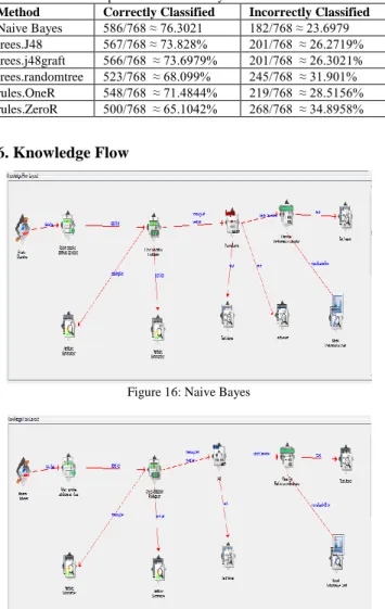
Table 9: Comparisons of Naive Bayes with other classifier Method Correctly Classified Incorrectly Classified Naive Bayes 586/768 ≈ 76.3021 182/768 ≈ 23.6979 trees.J48 567/768 ≈ 73.828% 201/768 ≈ 26.2719% trees.j48graft 566/768 ≈ 73.6979% 201/768 ≈ 26.3021% trees.randomtree 523/768 ≈ 68.099% 245/768 ≈ 31.901% rules.OneR 548/768 ≈ 71.4844% 219/768 ≈ 28.5156% rules.ZeroR 500/768 ≈ 65.1042% 268/768 ≈ 34.8958% 6. Knowledge Flow

Figure 16: Naive Bayes

Figure 17: J48

Figure 16 and Figure 17 shows the knowledge flow for diabetes using J48 and Naive Bayes. Knowledge flow can be used for data processing and analysis. Knowledge flow can either handle data in batches or incremental form. Knowledge flow can handle incremental updates with processing nodes which can load and pre-process individual instances before feeding them into appropriate learning algorithms. It also provides nodes for visualization and evaluation of incremental data. Once the

set of interconnected nodes has been configured, loaded and run properly, it can be saved for later re-use.

7. Conclusion

In this paper, we have used data sets for diabetes disease from the machine learning laboratory at the University of California Irvine. All the patients data are trained and tested using 10 cross validation with Naive Bayes and J48, and then the performance were evaluated, investigated and compared with other classification algorithms using WEKA. The results predicted that the best algorithm is Naive Bayes with an accuracy of 76.3021% correctly classified and 23.6979 incorrectly classified and followed with J48 with an accuracy of 73.8281% correctly classified and 26.2719% incorrectly classified. Also refer to figure16 and figure 17; we see the knowledge flow of Naive Bayes and J48 which shows step by step graphical user interface on how we carried out the algorithms.

8. Future Work

There is a chance of improving the performance of Pima Indian Diabetes and future work could concentrate on the following:

 If we use filters classifier for both supervised and unsupervised learning.

 If we apply cost sensitive evaluation for our data sets might make the study more practical and valuable.

 In this survey we used only 6 classification algorithms but if the number of rules are increased number of rules we could get more accurate diagnosis results.

Acknowledgement

I would like to thank almighty and my family for their constant support during this work. I would also like to thank my supervisors Dr. Anael Sam from Nelson Mandela African Institute of Science and Technology, Dr. Yaw Nkansah-Gyekye from Nelson Mandela African Institute of Science and Technology and Dr. Muhammad Abulaish from Jamia Milia Islamia for their guidance and valuable support during this work.

References

[1] Buse, JB., Ginsberg, HN. (2007). "Primary Prevention of cardiovascular disease in people with diabetes mellitus." A scientific statements from the American Heart Association and the American Diabetes Association. pp.162-172.

[2] International Diabetes Federation (IDF) atlas data, http://www.diabetesatlas.org

[3] Diabetes in America 2nd Edition, http:// diabetes.niddk.nih.gov/dm/pubs/america/pdf, 221-233

[4] Barakat, NH., Bradley, AP., Barakat, MN. (2010).“Intelligible Support Vector Machines for diagnosis of

(9)

Diabetes Mellitus.” IEEE Transactions on Information Technology in Biomedicine 14( 4), pp.1114-1120.

[5] Rong-Ho, Lin. (2009). “An intelligent model for liver diseases diagnosis”. Artificial Inteligence in medicine 47, pp.53-62.

[6] Jaree, Thongkam., Guandong, Xu., Yanchun, Zhang., Fuchun, Huang. (2008). "Breast Cancer Survivability via AdaBoost Algorithms" Second Australian Workshop on Health Data and Knowledge Management.

[7] Cortes, C. Vapnik V. (1995) “Support-vector networks”, Machine Learning, 20(2),pp. 273-297.

[8] Herron, P. (2005). “Machine Learning for Medical Decision Support: Evaluating Diagnostic Performance of Machine Learning Classification Algorithms”, INLS 110, Data Mining. [9] Balakrishnan, Sarojini., Narayanasamy, Ramaraj., Savarimuthu, Nickolas. (2009) “Enhancing the Performance of LibSVM Classifier by kernel F-Score Feature Selection”, Contemporary Computing, Volume 40, Part 10, pp. 533-543. [10] Andreassen, S., Benn, J. J., Hovorka, R., Olesen, K. G., Carson, E. R. (1994) "A probabilistic approach to glucose prediction and insulin dose adjustment: description of metabolic model and pilot evaluation study", Computer Methods and Programs in Biomedicine, 41(3-4) pp.153-65

[11] Manish, Jain.(2009). "Data Mining: Typical Data Mining Process for Predictive Modeling" BPB Publications. pp.235-241. [12] Liao SH (2003). "Knowledge Management Technologies and applications Literature review from 1995 to 2002", Expert System with Application, 25, pp155-164.

[13] Wah, TY., Abu, Bakar, Z. (2003). "Investigating the Status of Data Mining in Practice". CiteSeerx College of Information Science and Technology Pennsylvania State University.

[14] Witten, IH., Eibe, Frank. (2011) "Data Mining: Practical Machine Learning Tools and Techniques, Second Edition (Morgan Kaufmann Series in Data Management Systems)" , pg 189-303.

[15] Wei, Fan., Albert, Bifet. (2013). "Mining Big Data: Current Status, and Forecast to the Future", SIGKDD Explorations Volume 14, Issue 2.

[16] Kumari, AV., Chitra, R. (2013). " Classification Of Diabetes Disease Using Support Vector Machine" International Journal of Engineering Research and Applications(IJERA) Vol. 3, Issue 2, pp.1797-1801.

[17] Magudeeswaran, G., Suganyadevi, D. (2013). " Forecast of Diabetes using Modified Radial basis Functional Neural Networks" International Conference on Research Trends in Computer Technologies (ICRTCT ) Proceedings published in International Journal of Computer Applications (IJCA) (0975 – 8887)

[18] Karegowda, AG., Jayaram, MA., Manjunath, AS. (2012). "Cascading K-means Clustering and K-Nearest Neighbor Classifier for Categorization of Diabetic Patients" International Journal of Engineering and Advanced Technology (IJEAT) ISSN: 2249 – 8958, Volume-1, Issue-3.

[19] UCI repository of bioinformatics Databases, Website: http://www.ics.uci.edu/~mlearn/MLRepository.html.

Salim Amour Diwani received his BS degree in computer science at Jamia Hamdard University, New Delhi, India in 2006 and Ms degree in computer science at Jamia Hamdard University in New Delhi, India in 2008. He is currently a PhD scholar in Information Communication Science and Engineering at Nelson Mandela African Institution of

Science and Technology in Arusha, Tanzania. His primary research interests are in Data Mining, Machine Learning and Database Management Systems. He published two papers in the area of Data Mining.