Murray State's Digital Commons
Murray State's Digital Commons
Murray State Theses and Dissertations Graduate School
2020
Evaluating an Ordinal Output using Data Modeling, Algorithmic
Evaluating an Ordinal Output using Data Modeling, Algorithmic
Modeling, and Numerical Analysis
Modeling, and Numerical Analysis
Martin Keagan Wynne BrownMurray State University
Follow this and additional works at: https://digitalcommons.murraystate.edu/etd
Part of the Analysis Commons, Applied Statistics Commons, Numerical Analysis and Computation Commons, Other Applied Mathematics Commons, Other Mathematics Commons, Other Statistics and Probability Commons, Probability Commons, and the Statistical Models Commons
Recommended Citation Recommended Citation
Brown, Martin Keagan Wynne, "Evaluating an Ordinal Output using Data Modeling, Algorithmic Modeling, and Numerical Analysis" (2020). Murray State Theses and Dissertations. 168.
https://digitalcommons.murraystate.edu/etd/168
This Thesis is brought to you for free and open access by the Graduate School at Murray State's Digital Commons. It has been accepted for inclusion in Murray State Theses and Dissertations by an authorized administrator of Murray State's Digital Commons. For more information, please contact [email protected].
Evaluating an Ordinal Output using Data Modeling,
Algorithmic Modeling, and Numerical Analysis
A Thesis Presented to
the Faculty of the Department of Mathematics and Statistics Murray State University
Murray, Kentucky
In Partial Fulfillment
of the Requirements for the Degree of Master of Science
by Martin Brown
Evaluating an Ordinal Output using Data Modeling,
Algorithmic Modeling, and Numerical Analysis
DATE APPROVED:
Dr. Donald Adongo, Thesis Advisor Dr. Christopher Mecklin, Thesis Advisor Dr. Manoj Pathak, Thesis Committee Dr. Maeve McCarthy, Graduate Coordinator, Jesse D. Jones College of Science, Engineering, and Technology
Dr. Claire Fuller, Dean, Jesse D. Jones College of Science, Engineering, and Technology
Dr. Robert Pervine, University Graduate Coordinator Dr. Timothy Todd, Provost
Acknowledgements
I would like to thank the Mathematics and Statistics Department at Murray State University for providing the most rewarding and interesting experience. So many individuals have influenced me in profound ways, and I would like to mention a few of them.
To Dr. Donald Adongo, thank you for making my transition to America as smooth as possible. I have enjoyed our long conversations in your office, and you have made me feel welcomed and comfortable at Murray State. Also, thank for your support in my classes and thesis. Your enthusiasm in helping students is something I will never forget.
To Dr. Christopher Mecklin, thank you for introducing me to machine learning. You helped me to discover my passion and develop grit. Also, thank you for your support in my thesis and being available at a moment’s notice to advise me during the tougher moments.
To Dr. Manoj Pathak, thank you for introducing me to the world of statistics; I did not know what I was missing. Also, thank you for your help during the thesis process.
To Claire Ghent, thank you for your help throughout my studies, and thank you for the endless grammer corrections and proof readings as well as bringing me tea during the writing process.
To my parents, Lindsay Brown and Elaine Brown, thank you for giving me the opportunity to study my Master’s degree. You have both supported and provided strong encouragement throughout all my endeavors. I could not be where I am today without your help.
Abstract
Data and algorithmic modeling are two different approaches used in predictive analytics. The models discussed from these two approaches include the proportional-odds logit model (POLR), the vector generalized linear model (VGLM), the clas-sification and regression tree model (CART), and the random forests model (RF). Patterns in the data were analyzed using trigonometric polynomial approximations and Fast Fourier Transforms. Predictive modeling is used frequently in statistics and data science to find the relationship between the explanatory (input) variables and a response (output) variable. Both approaches prove advantageous in different cases depending on the data set. In our case, the data set contains an output variable that is ordinal. Using grade records from Murray State University, the goal is to find the best predictive model that can implement an ordinal output by means of data modeling and algorithmic modeling.
To train the models, k-fold cross validation is used to find the optimal tuning parameters and performance for each of the models. The logarithmic loss (logLoss) performance metric is utilized to determine which method has the top predictive accuracy. A comparison of each statistical model and a look at alternative methods is discussed.
Contents
1 Introduction 1
2 Training and Testing 3
2.1 Logarithmic Loss . . . 4
2.2 K-Fold Cross Validation . . . 6
2.3 Training with the caret Package . . . 9
2.3.1 Cross Validation for POLR . . . 10
2.3.2 Cross Validation for the Vector Generalized Linear Model . . . 11
2.3.3 Cross Validation for CART . . . 12
2.3.4 Cross Validation for Random Forests . . . 15
3 Proportional-Odds Logistic Regression 17 3.1 Implementing POLR in R . . . 19
3.2 Prediction and logLoss for POLR . . . 23
4 Vector Generalized Linear Model 24 4.1 Implementing VGLM in R . . . 26
4.2 Prediction and logLoss for VGLM . . . 28
5 Classification and Regression Tree Model 29 5.1 Implementing CART inR . . . 33
5.2 Prediction and logLoss for CART . . . 36 v
6 Random Forests Model 37
6.1 Implementing Random Forests in R . . . 40 6.2 Prediction and logLoss for Random Forests . . . 41
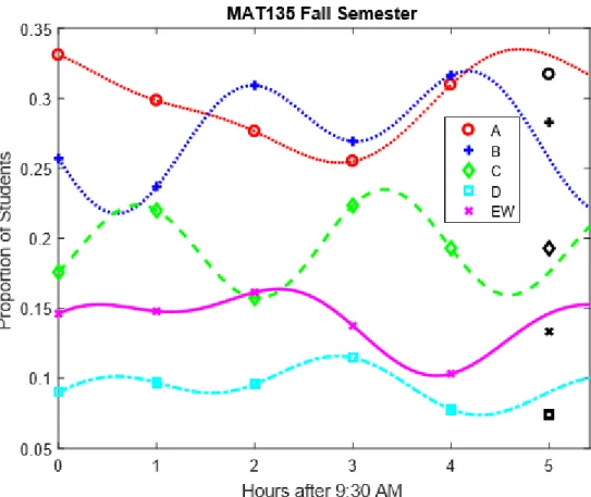
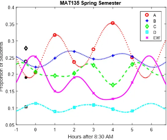
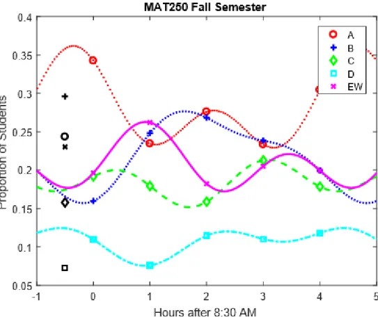
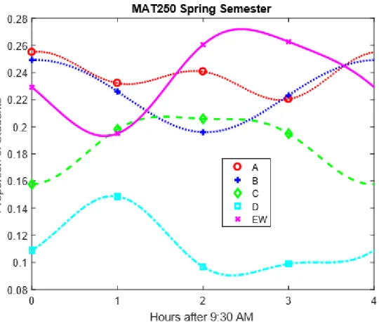
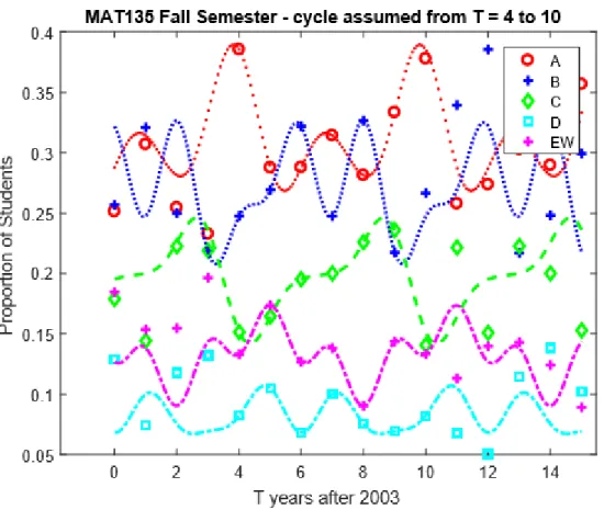
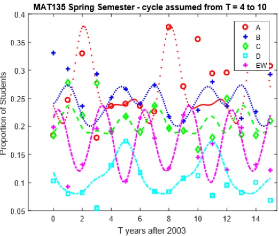
7 Trigonometric Functions and Fourier Series 42
7.1 Implementing Trigonometric Functions in
M AT LAB for the Start Times . . . 44 7.2 Implementing Trigonometric Functions in
M AT LAB for the Years Since 2003 . . . 49
8 Comparing the Models 54
Appendices 57
A R Code for Training and Testing 57
A.1 Data Set Up . . . 57 A.2 Training the Models Code . . . 58
B R Code for POLR 62
C R Code for VGLM 63
D R Code for CART 64
E R Code for Random Forests 65
F M AT LAB Code for Trigonometric Polynomials 66
1
Chapter 1
Introduction
Leo Breiman [1] explains that statistical modeling can be split into two different cultures, data modeling and algorithmic modeling. Breiman uses the analogy of a black box that generates the data, where inputs, Xi for some i, enter the black
box producing the output, Y. Data modeling involves making assumptions for the internals of the black box then builds a model based on these assumptions. This is the approach that statisticians traditionally employ. Algorithmic modeling treats the internal nature of the black box as unknown and alternatively finds an algorithm that takes the inputs to predict the output based on patterns found in the data.
Questions on prediction are more prevalent than ever. From using relevant factors to predict consumer shopping habits to using relevant factors to predict if a person has diabetes, we are able to answer more questions with the ever-increasing amount of data. The main goal of this thesis is to determine the best model, in terms of predictive accuracy, that predicts an ordinal output. In our case, the output variable is student grades collected from two different courses offered by the mathematics and statistics department at Murray State University. Specifically, the models are chosen to deal with the ordinal output variable commonly referred to in supervised machine learning as classification. In addition, we combine the fields of statistics, machine learning, and numerical analysis to evaluate our ordinal data. As important
2 as accuracy is, a discussion on the interpretability of each model is included because an explanation of results is important when including a non-technical audience.
The arrangement of this thesis begins in chapter 2 with a description of the data used as well as an introduction of the concepts of the logarithmic loss perfor-mance metric (logLoss) and k-fold cross validation (kFCV). In chapter 3, we begin determining the best method to prognosticate student grades with a detailed descrip-tion of the propordescrip-tional-odds logistic regression model (POLR). In chapter 4, the vector generalized linear model (VGLM) is considered to evaluate the proportionality of our data set. In chapter 5 and 6, we investigate the classification and regression tree (CART) model and the adapted random forests model (RF), respectively. In chapter 7, a numerical anaylsis study is introduced using trigonometric approximation poly-nomial and Fourier series to analyze the trends in the data. Lastly, a comparison of the methods is discussed and an examination into further methods for potential use is conducted in chapter 8.
3
Chapter 2
Training and Testing
In this thesis, the goal is to predict student grades obtained from data records from Murray State University and compare the best predictive model for the ordinal output. The output variable of student grades is ordinal, which Fox et al. [2] describes this as categories that have a natural order. This is different from multinomial data, where the data set is categorical but does not have an intrinsic order. An example of multinomial would be a person’s favorite color such as green, blue, or red.
This study omits students who have audited a course and combines the students who have received the grade E and who withdrew from the course with a W on their transcript. Therefore, the data set used throughout the thesis contains an ordered factored output variable as displayed in (G). Models involving this type of output are referred to as multi-class classification problems.
EW < D < C < B < A. (G)
The input variables in consideration are:
• ‘Semester’: a factor indicating if the class was held in ‘Spring’ or ‘Fall’; • ‘StartTime’: a factor indicating the start time of the class;
2.1. Logarithmic Loss 4
• ‘YrSince2003’: a number indicating how many years since 2003 that the class
was taught;
• ‘Class’: a factor indicating if the class is Introduction to Probability and
Statis-tics ‘MAT135’ (called ‘STA 135’ since 2016), or, Calculus and Analytic Geom-etry I ‘MAT250’,
• ‘Day’: a number indicating the number of days a week that the class meets.
With all the different models, we require a performance metric to be able to determine which method is best suited for predicting student grades (G). The logLoss function is a consistent metric that deals well with multi-class classification problems [3] and can be utilized in areas from machine learning to numerical analysis. Since we cannot wait for a new set of data to test the model without waiting for months or years, we require the data set to be split into a training set and a testing set in an attempt to prevent the models from overfitting the data. The model will be performed on the training set and validated on the testing set, which is a completely seperate portion of the data set and is not used in the training set.
To train the model, we perform k-fold cross validation demonstrated in chapter 2.2. To train our model and calculate the logLoss metric, we use the ‘caret’ package [11] in the statistical program R. M AT LAB is used to implement the trigonometric polynomials.
2.1
Logarithmic Loss
Logarithmic loss, or commonly referred to as logLoss, is a metric that penalizes the false classifications given by a model. This works especially well for multi-class classification where the method assigns a probability to each of the classes for all observations [3]. Therefore, the logLoss function was chosen over traditional accuracy metrics because we are not predicting a binary response. Let M be the number of
2.1. Logarithmic Loss 5 classes in the data set and let N be the number of observations belonging to our classes M. In our case, we have M = 5 classes in (G), and we have N = 1760 observations. Then, the logLoss function is given by
logLoss=− 1 N N X i=1 M X j=1 yijln(pij), (2.1.1)
where yij ={0,1} indicates if observation i belongs to class j, and pij indicates the
probability of observationibelonging to class j [3]. Also,ln refers to the natural log. Note that the logLoss will only contain the summation of misclassified observations and will heavily penalize the observations that were confident and incorrect [5]. A model that perfectly predicts student grades (G) will have a logLoss of zero therefore, the logLoss takes on values [0,∞), i.e. no upper bound. A model with higher accuracy has a logLoss closer to zero thus, we must minimize the logLoss to improve the accuracy of our model.
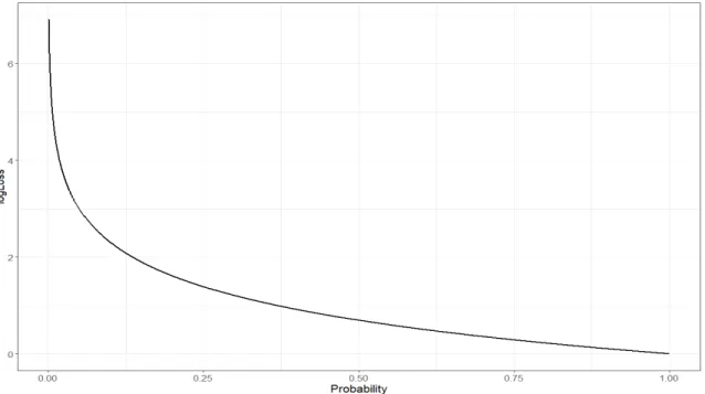
Figure 2.1.1: Plot of logLoss against predicted probability
In figure 2.1.1, the predicted probability is zero for incorrect predictions and one for correct predictions. The logLoss gradually decreases as the predicted probabil-ity increases, and on the left of figure 2.1.1, its apparent that the model is heavily
2.2. K-Fold Cross Validation 6 penalized on making confident incorrect predictions.
Since we have M = 5 classes, we can calculate the “dumb” or non-informative logLoss for our classification problem [6]. This is the same as assuming that students’ grades are uniformly distributed, where each grade has a 20% chance of occuring. Hence, the “dumb” logLoss value is
logLoss=−ln 1 M =−ln1 5 =ln(5) = 1.6094.
We can compare the subsequent models to the uniform distribution of the grades (G), which has a logLoss of 1.609437912. Since the distribution of grades is not exactly uniform, as certain grades are more prevalent and others less prevalent in the actual data, the “dumb” logLoss for grade predictions will be slightly less thanln(5). Let us consider a situation when there are 15% A grades, 30% B grades, 25% C grades, 10% D grades and 20% EW grades. Then, the non-informative logLoss can be calculate using the entropy function (5.0.2), which will be defined in chapter 5.
logLoss=−(0.15ln(0.15) + 0.30ln(0.30) + 0.25ln(0.25) + 0.10ln(0.10) + 0.20ln(0.20)),
= 1.5448.
2.2
K-Fold Cross Validation
The code for processing the data set is in appendix A.1. Firstly, we split the data into a training and testing set. Secondly, we converted this “wide” formated data, which had a column for each of the grades (G), to a “long” format, where we created a column of grades, ‘Grade’, along with a column of frequencies of each grade, ‘Freq’. Lastly, uncounting the frequencies for each grade, we extended the data to the “longest” format. The cross validation will be performed on the “longest” training set, ‘Grades.training’, and the model will be tested on the “longest” testing set,
2.2. K-Fold Cross Validation 7 ‘Grades.testing’. Overall, we are going from a “wide” format, where each section of a class is represented by a single row, to a “long” format, where each section is represented by five rows, one for each of the grades. Then, we converted the “long” format to the “longest” format, where each section is represented by a number of rows that is equivalent to the number of students in that class. The “longest” format is useful to fit the models, make predictions, and correctly compute the logLoss using the built-in R function.
Our goal is to find a method that predicts student grades (G), minimizes the overall logLoss, and is better than just assuming a uniform distribution to make random predictions. The main objective of cross validation is to use our training set, which is separate from the testing set, and create folds within the training set to train our model and find the optimal model provided certain tuning parameters. A training set is one in which the model is constructed, and the testing set is used to test the validity of the model given the optimal tuning parameters. To begin, the test error is the average error that results from using a statistical or machine learning method to predict the response on a new observation [8]. This is the error produced from using a model on the training set. The test error is the logLoss metric defined in chapter 2.1. Cross validation estimates the testing error by performing the logLoss on the folds from the training set. However, we require a large enough training set to perform the methods but equally a large enough testing set to validate. We separated the full data set into a 2/3-rds portion for the training set, called ‘Grades.training’, and the remaining 1/3-rd portion for the testing set, called ‘Grades.testing’. This is shown in the R code in appendix A.1. The splitting was performed on the “wide” data set in order to keep all the students in a particular section of a class together, and then the processing from “wide” to “long” to “longest” was performed after sectioning off a training set and testing set.
2.2. K-Fold Cross Validation 8 refers to the number of partitions or folds that the data is split into [8]. It works by randomly dividing the data set into 1k approximately equally spaced portions. The
k-th fold is used as the validation set that is used to estimate the testing error, and all but the k-th fold is used as the training set in which the model is fitted on. A common choice for k, and used in this thesis, is k = 10. In our case, 10% of the data is used as the validation set, and the remaining 90% is used to fit a model. This is a good compromise to leave-one-out-cross-validation (LOOCV), where k will be equal to leaving out one observation with replacement and fitting a model, i.e. k =n, which is computationally expensive.
Each fold produced is a different iteration, and at each iteration the logLoss values
logLoss1, . . . , logLossk are calculated, which is the testing error for each fold. For k = 10 folds, the 10-fold cross validation estimate, [8], is the average of the values
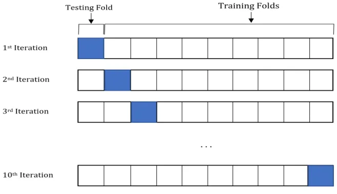
logLossi for all i= 1,2, . . . ,10: CV(k) = 1 10 10 X k=1 logLossk, = 1 10 10 X k=1 − 1 N N X i=1 M X j=1 yij,kln(pij,k) ! . (2.2.1) As illustated in figure 2.2.1, we seek = 10 fold cross validation splits the data into a validation set,k = 1, and uses the remaining k = 9 as the training set. In the first iteration, the first fold in blue indicates the validation set. In the second iteration, the second fold in blue is used as the validation set; this is repeated until we use all the folds as the validation set. This is used to create a logLoss value at each iteration on each validation set leading to equation (2.2.1).
2.3. Training with the caret Package 9
Figure 2.2.1: Demonstration of k = 10 fold cross validation
To implement cross validation, we require the use of a statistical program R. In particular, Kuhn et al. [11] created the ‘caret’ package which contains the functions ‘trainControl’ and ‘train’. Using these functions, we can train the models to find the minimum logLoss values for a certain tuning parameter associated with the model.
2.3
Training with the caret Package
This section accompanies the R code in section A.2. As mentioned before, we arbitrarily split our data set into a training set by randomly selecting two thirds of the data set. Then cross validation was preformed on the POLR model, followed by the VGLM model, the CART model, and then the RF model. The optimal tuning parameters will be used on the testing set in the subsequent chapters, and the logLoss of the tested model will be calculated. Cross validation will only be performed on the statistical study.
2.3. Training with the caret Package 10
2.3.1
Cross Validation for POLR
Using the ‘train’ function from the ‘caret’ package, we can find the minimum logLoss value for the proportional-odds logistic regression model. Within the ‘train’ function we usemethod=polrto train the model on the tuning parameters. We can train the model based on the type of regression model we should use; in other words, the tuning parameter is distinguishing which model is best between using a logistic regression model,logistic, or using a normal distribution probit model. Equivalently, this is determining if we should use a logit link or a probit link, respectively. These distributions were chosen because of work done by Fox [14] comparing the two distri-butions. TheR output of ‘train.polr’ is given below.
> p r i n t ( t r a i n . p o l r ) O r d e r e d L o g i s t i c or P r o b i t R e g r e s s i o n 7 7 0 3 s a m p l e s 6 p r e d i c t o r 5 c l a s s e s : ‘ EW ’ , ‘ D ’ , ‘ C ’ , ‘ B ’ , ‘ A ’ No pre - p r o c e s s i n g R e s a m p l i n g : Cross - V a l i d a t e d (10 f o l d ) S u m m a r y of s a m p l e s i z e s : 6934 , 6933 , 6933 , 6931 , 6932 , 6931 , ... R e s a m p l i n g r e s u l t s a c r o s s t u n i n g p a r a m e t e r s : m e t h o d l o g L o s s l o g i s t i c 1 . 5 5 0 8 4 4 p r o b i t 1 . 5 5 0 8 7 6
l o g L o s s was u s e d to s e l e c t the o p t i m a l m o d e l u s i n g the s m a l l e s t v a l u e .
The f i n a l v a l u e u s e d for the m o d e l was m e t h o d = l o g i s t i c .
As seen above, logLoss was used to select the optimal model using the smallest value. In this case, the optimal model is using logistic regression with a logLoss value of 1.550844. The probit link has a logLoss value that agrees up to about 1.5508 (four decimal places), but we chose the method that produces the slightly lower logLoss while also taking into consideration the interpretability of the model. Fox [14] states
2.3. Training with the caret Package 11 that the advantages of using logistic over probit is that it is simpler and easier to work with, since the CDF is very simple and we do not have to evaluate an integral, and the logistic inverse transformation is directly interpretable as odds, which will be defined in the next chaper. To summarize, student grades (G) follow a logistic distribution where we can use alogit link for the POLR model.
2.3.2
Cross Validation for the Vector Generalized Linear Model
Alternatively, we have the cumulative probability model for ordinal data, or ref-ered to as the vector generalized linear model. We can train this model to find the optimal model based on the type of link used, such as logit, probit, cloglog,cauchit, orlogclink. This is almost the same as the POLR model, but we are considering more possibilities for the link function with the VGLM model. Furthermore, we trained each of these links based on whether we include the parallelism assumption, which Yee in [15] states this as determining if the data follows a parallel assumption − if the data set has proportional odds, i.e. specifying if the estimated coefficients of the VGLM model have equal/unequal coefficients. Further explanation on the par-allelism assumption and the tuning parameter parallel can be found in chapter 4. In R, we use the ‘train’ function with method = vglmCumlative to train the link and parallel assumption, which is implemented by either setting parallel = T RU E
orparallel =F ALSE. TheR output of ‘train.vglm’ is given below.
> p r i n t ( t r a i n . v g l m ) C u m u l a t i v e P r o b a b i l i t y M o d e l for O r d i n a l D a t a 7 7 0 3 s a m p l e s 6 p r e d i c t o r 5 c l a s s e s : ‘ EW ’ , ‘ D ’ , ‘ C ’ , ‘ B ’ , ‘ A ’ No pre - p r o c e s s i n g R e s a m p l i n g : Cross - V a l i d a t e d (10 f o l d ) S u m m a r y of s a m p l e s i z e s : 6932 , 6933 , 6933 , 6933 , 6934 , 6933 , ... R e s a m p l i n g r e s u l t s a c r o s s t u n i n g p a r a m e t e r s :
2.3. Training with the caret Package 12 p a r a l l e l l i n k l o g L o s s F A L S E l o g i t 1 . 5 5 1 3 7 8 F A L S E p r o b i t 1 . 5 5 1 4 2 9 F A L S E c l o g l o g 1 . 5 5 1 5 2 6 F A L S E c a u c h i t 1 . 5 5 1 3 4 8 F A L S E l o g c 1 . 5 5 1 4 2 0 T R U E l o g i t 1 . 5 5 0 8 7 6 T R U E p r o b i t 1 . 5 5 0 8 6 8 T R U E c l o g l o g 1 . 5 5 2 8 9 2 T R U E c a u c h i t 1 . 5 5 3 2 0 8 T R U E l o g c 1 . 5 5 2 9 2 0
l o g L o s s was u s e d to s e l e c t the o p t i m a l m o d e l u s i n g the s m a l l e s t v a l u e .
The f i n a l v a l u e s u s e d for the m o d e l w e r e p a r a l l e l = TRUE , and l i n k = p r o b i t .
As we can see above, the optimal VGLM model has a logLoss value of 1.550868 with parallel =T RU E with a probit link. Again, the probit and logit links are very similar in terms of logLoss, so we will use a logit link as it is more interpretable and is commonly used in data modeling. This is almost exactly the same logLoss value of the POLR model with the same link and assumption of parallelism. These models are very similar but the implementation is slightly different: the POLR model uses maximum likelihood estimates and the VGLM model uses matrices. We can deduce by cross validation that both the POLR and VGLM model fit a proportional-odds model. Note that under the parallel assumption, each of the links trained above have a logLoss value that agree up to about 1.55 (two decimal places), which indicates that the link chosen is arbitrary. To summarize, we will use a logit link and the parallel assumption, parallel=T RU E.
2.3.3
Cross Validation for CART
Similarly, using the ‘train’ function we can find the optimal parameters of the CART method. Firstly, using method = rpart we can find the best complexity parameter, cp. Secondly, using method= rpart1SE we can find the optimal model using the one-standard error method [12]. Lastly, we canl find the optimal maxdepth
2.3. Training with the caret Package 13 for the classification tree holding the cp value constant at the value we deduce from
method = rpart. The maximum classification tree depth, maxdepth, is the tuning parameter that controls the maximum depth of the terminal nodes. An explanation of each of the tuning parameters and the CART model can be found in chapter 5. To start, we let the ‘train’ function find the optimal cp value from 100 randomly selected cp values by setting tuneLength = 100. We have the following results for ‘train.rpart’, leaving out most of the cp values explored.
> p r i n t ( t r a i n . r p a r t ) C A R T 7 7 0 3 s a m p l e s 6 p r e d i c t o r 5 c l a s s e s : ‘ EW ’ , ‘ D ’ , ‘ C ’ , ‘ B ’ , ‘ A ’ No pre - p r o c e s s i n g R e s a m p l i n g : Cross - V a l i d a t e d (10 f o l d ) S u m m a r y of s a m p l e s i z e s : 6932 , 6933 , 6933 , 6933 , 6934 , 6933 , ... R e s a m p l i n g r e s u l t s a c r o s s t u n i n g p a r a m e t e r s : cp l o g L o s s 1 . 1 8 9 9 2 5 e -03 1 . 5 5 5 7 6 4 1 . 2 3 2 4 2 3 e -03 1 . 5 5 5 4 3 7 1 . 2 7 4 9 2 0 e -03 1 . 5 5 5 4 3 7 1 . 3 1 7 4 1 7 e -03 1 . 5 5 5 4 5 0 1 . 3 5 9 9 1 5 e -03 1 . 5 5 5 3 4 0 1 . 4 0 2 4 1 2 e -03 1 . 5 5 4 8 3 7 1 . 4 4 4 9 0 9 e -03 1 . 5 5 4 5 1 3 1 . 4 8 7 4 0 7 e -03 1 . 5 5 5 0 4 6 1 . 5 2 9 9 0 4 e -03 1 . 5 5 5 0 8 4 1 . 5 7 2 4 0 2 e -03 1 . 5 5 4 6 4 6 1 . 6 1 4 8 9 9 e -03 1 . 5 5 4 5 7 1 1 . 6 5 7 3 9 6 e -03 1 . 5 5 4 5 7 1 1 . 6 9 9 8 9 4 e -03 1 . 5 5 4 5 7 1 1 . 7 4 2 3 9 1 e -03 1 . 5 5 4 7 7 7 1 . 7 8 4 8 8 8 e -03 1 . 5 5 5 0 3 7 1 . 8 2 7 3 8 6 e -03 1 . 5 5 0 8 9 0 1 . 8 6 9 8 8 3 e -03 1 . 5 5 0 8 9 0 1 . 9 1 2 3 8 0 e -03 1 . 5 5 1 6 4 5 1 . 9 5 4 8 7 8 e -03 1 . 5 5 1 6 4 5 1 . 9 9 7 3 7 5 e -03 1 . 5 5 1 6 4 5
2.3. Training with the caret Package 14
l o g L o s s was u s e d to s e l e c t the o p t i m a l m o d e l u s i n g the s m a l l e s t v a l u e .
The f i n a l v a l u e u s e d for the m o d e l was cp = 0 . 0 0 1 8 6 9 8 8 3 .
The ‘train’ function deduces that the optimal model used a complexity parameter value of 0.001869883 with a logLoss of 1.550890.
Hastie et al. [13] states that the one-standard error method is a rule used with cross validation: which is used we to choose the most parsimonious model whose error is no more than one standard error above the error of the best model. This can be applied to finding the optimal cp value, where we find the one-standard error threshold of the logLoss values. Therefore, usingmethod=rpart1SE we get a logLoss value of 1.558576 with complexity parameter of 0, which tells us that using the one-standard error method to deduce the cp value is not as accurate as using a cp of 0.001869883. In chapter 5, we will see that a cp of 0 will allow the classification tree to grow until there are only a few observations left in each node, which is not helpful in making predictions.
Now, we can train the CART model to find the maximum tree depth, maxdepth, controlling for a cp of 0.001869883. Usingmethod=rpart2 in the ‘train’ function, we can find the optimal classification tree depth. The logLoss value for all tree depths ranging from two to 30 produced a logLoss of 1.558576. This tells us that tuning for maxdepth is arbitrary, and since we want an interpretable tree that is not too big, we will use maxdepth = 5 in R. We will see in chapter 5 that the complexity parameters greater than zero control the tree depth. This is the reason the logLoss for the maxdepth does not change for cp = 0.001869883. The R code for maxdepth
training can be found in A.2. To summarize, we will use a cp of 0.001869883 with
2.3. Training with the caret Package 15
2.3.4
Cross Validation for Random Forests
The last of our machine learning models is the random forest. The tuning pa-rameters involved are mtry and num.trees. Briefly, the tuning parameter mtry is the number of input variables to possibly split in each node in the classification tree, and num.treesis the total number of classification trees grown by the random forest model. The tuning parametersplitruleis held constant with “gini” to implement the Gini index splitting criterion 5.0.1 described in chapter 5. Also, the tuning parameter
min.node.size is held constant at one so that the minimum number of observations that can remain in a terminal node is a single observation. A detailed explanation of each tuning parameter is included in chapters 5 and 6.
Firstly, using method = ranger in the ‘caret’ package and holding splitrule = “gini” and min.node.size= 1 constant, we can train for the tuning parameter mtry, producing the following R output for ‘train.rf’.
> p r i n t ( t r a i n . rf ) R a n d o m F o r e s t 7 7 0 3 s a m p l e s 6 p r e d i c t o r 5 c l a s s e s : ‘ EW ’ , ‘ D ’ , ‘ C ’ , ‘ B ’ , ‘ A ’ No pre - p r o c e s s i n g R e s a m p l i n g : Cross - V a l i d a t e d (10 f o l d ) S u m m a r y of s a m p l e s i z e s : 6932 , 6933 , 6933 , 6933 , 6934 , 6933 , ... R e s a m p l i n g r e s u l t s a c r o s s t u n i n g p a r a m e t e r s : m t r y l o g L o s s 2 1 . 5 4 1 9 4 7 3 1 . 5 4 3 0 0 3 4 1 . 5 5 1 2 7 2 5 1 . 5 6 3 0 0 8 6 1 . 5 7 5 7 1 4 T u n i n g p a r a m e t e r ’ s p l i t r u l e ’ was h e l d c o n s t a n t at a v a l u e of g i n i T u n i n g p a r a m e t e r ’ min . n o d e . s i z e ’ was h e l d c o n s t a n t at a v a l u e of 1 l o g L o s s was u s e d to s e l e c t the o p t i m a l m o d e l u s i n g the s m a l l e s t v a l u e .
2.3. Training with the caret Package 16
The f i n a l v a l u e s u s e d for the m o d e l w e r e m t r y = 2 , s p l i t r u l e = gini , and min . n o d e . s i z e = 1.
As shown above, an optimal random forest model usesmtry= 2 with a minimum logLoss value of 1.541947. In other words, for each node there will be only two random input variables available to split the node.
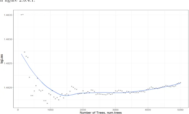
Secondly, holding splitrule= “gini”,min.node.size= 1, and mtry= 2 constant, we can use the training set to build 100 different random forests, increasing the tuning parameternum.treesto find the minimum logLoss value. The results are summarised in figure 2.3.4.1.
Figure 2.3.4.1: Plot to find the optimal total number of trees
The optimal random forests model will use num.trees = 1500, since in figure 2.3.4.1 the logLoss value is minimum around 1500 classification trees. To conclude, the final tuning parameters are mtry = 2 and num.trees = 1500. Chapter 8 will include a comparison of results of all the methods considered.
17
Chapter 3
Proportional-Odds Logistic
Regression
One possible data modeling approach for grade prediction is the proportional-odds logistic regression method (POLR). Models like POLR are designed for our output variable (G) which is ordered categorical responses [14]. Based on the definition obtained in [17], we define the POLR model below. Note that training from chapter 2 produced an optimal model using the logit link, which is implemented into the definition.
Definition. Let Y be an ordinal output variable with M classes, or referred to as categories. Then, the cumulative probability ofY less than or equal to a specific class level m= 1, . . . , M −1, is given byP(Y ≤m). Note thatP(Y ≤M) = 1. Then, the
odds, or ratio, of being less than or equal to a particular class is given by
P(Y ≤m)
P(Y > m). (3.0.1)
Now, the logit, or log odds, is given by
logit[P(Y ≤m)] =ln P(Y ≤m) P(Y > m) , =β0,m+β1,mX1+β2,mX2+· · ·+βk,mXk, (3.0.2)
18 We only consider the classes m= 1, . . . , M −1 since
P(Y > M) = 1−P(Y ≤M) = 1−1 = 0,
which will lead to undefined odds in equation (3.0.1). In our case, grades consists of
M = 5 classes with class levelsm = 1, . . . ,4, excluding m= 5 because P(Y ≤5) = 1. Hence, Y =
level 1, if the grade is an EW, level 2, if the grade is a D or lower, level 3, if the grade is a C or lower, level 4, if the grade is a B or lower, level 5, if the grade is an A or lower.
(3.0.3) In other words, for grades EW, D, C, B, and A we have Y = 1,2,3,4, and 5, re-spectively. It makes sense that P(Y ≤5) = 1 since this equates to the probability of getting an A or lower, which will always be one.
The POLR method intuitively has a proportional-odds assumption between each class in the output. In equation (3.0.2), the proportional odds assumption, or par-allel regression assumption [17], describes the coefficients, βi,m for i = 1,2, . . . , k,
of the logit model as being the same at each class level. Or, the odds between each cumulative probability link is equal. Therefore, equivalently equation (3.0.2) becomes
logit[P(Y ≤m)] =β0,m+β1X1+β2X2 +· · ·+βkXk. (3.0.4)
Using the ‘MASS’ package [19], we can fit the POLR model using the function ‘polr’. As a generalized notation cannot be reached, R uses the following logit format from [17]:
logit[P(Y ≤m)] =β0,m−η1X1 −η2X2− · · · −ηkXk,
3.1. Implementing POLR in R 19 Here, we see that −ηi = βi for i = 1,2, . . . , k, where ζm is used to represents the
intercepts, and η is used to represent the estimated coefficients. The η estimated coefficients can be calculated using maximum likelihood estimates, which are imple-mented in R. To find the inverse of the logit link function, we begin by setting
logit[P(Y ≤m)] = loge P(Y≤m) 1−P(Y≤m) =ζm−η, then, ln P(Y ≤m) 1−P(Y ≤m) =ζm−η, P(Y ≤m) 1−P(Y ≤m) =e ζm−η, P(Y ≤m) = e ζm−η 1 +eζm−η, P(Y ≤m) = 1 1 +e−(ζm−η).
Finally, we get logit−1[P(Y ≤m)] =P(Y ≤m) = 1/(1 +e−(ζm−η)). From the inverse
logit, we can find out the probability of a getting a certain grade or below based on the levels (7.0.1). Additionally, we can exponentiate both sides of equation (3.0.5) to get
P(Y ≤m)
1−P(Y ≤m) =exp[ζm−η],
=exp(ζm)exp(−η). (3.0.6)
The ratio (3.0.6) is the called the odds. We observe that the POLR model is an additive model using (3.0.5) but also a multipicative model for the odds, as seen in the ratio (3.0.6), [14].
3.1
Implementing POLR in
R
Using the ‘MASS’ package [19], we can implement proportional odds logistic regression where the R code can be found in appendix B. We can now use the
3.1. Implementing POLR in R 20 ‘Grades.testing’ portion of the data set, which is the portion the data set meant for testing and is seperate from the training set to avoid overtraining. This is used to obtain an accurate comparison of the models later. The following output are the results from the ‘polr’ function, which I defined in R as ‘Grades.polr’.
> s u m m a r y ( G r a d e s . p o l r ) C a l l : p o l r ( f o r m u l a = G r a d e ~ S e m e s t e r + S i z e + S t a r t T i m e + Day + C l a s s + Y r S i n c e 2 0 0 3 , d a t a = G r a d e s . testing , H e s s = TRUE , m e t h o d = " l o g i s t i c " ) C o e f f i c i e n t s : V a l u e Std . E r r o r t v a l u e S e m e s t e r S p r i n g - 0 . 1 2 3 2 5 0 . 0 5 9 2 8 6 -2.0789 S i z e 0 . 0 1 1 8 7 0 . 0 0 6 7 7 6 1 . 7 5 1 8 S t a r t T i m e 0 8 :30 - 0 . 3 8 5 2 6 0 . 3 4 7 0 0 3 -1.1102 S t a r t T i m e 0 9 :30 - 0 . 2 2 2 2 8 0 . 3 4 0 1 8 5 -0.6534 S t a r t T i m e 1 0 :30 - 0 . 1 2 7 4 8 0 . 3 4 4 2 1 5 -0.3703 S t a r t T i m e 1 1 :30 - 0 . 1 1 4 5 3 0 . 3 4 2 2 0 0 -0.3347 S t a r t T i m e 1 2 :30 - 0 . 1 2 9 0 9 0 . 3 4 6 5 5 2 -0.3725 S t a r t T i m e 1 3 :30 - 0 . 0 7 8 6 4 0 . 3 4 5 1 9 6 -0.2278 S t a r t T i m e 1 4 :30 - 0 . 2 0 3 2 6 0 . 3 0 3 3 8 1 -0.6700 Day 0 . 1 3 2 1 3 0 . 2 3 8 4 6 9 0 . 5 5 4 1 C l a s s M A T 2 5 0 - 0 . 1 8 1 1 9 0 . 2 4 8 1 6 3 -0.7301 Y r S i n c e 2 0 0 3 0 . 0 2 8 5 1 0 . 0 0 6 3 4 4 4 . 4 9 5 1 I n t e r c e p t s : V a l u e Std . E r r o r t v a l u e EW | D -0.6259 0 . 8 9 5 8 -0.6987 D | C -0.0833 0 . 8 9 5 7 -0.0930 C | B 0 . 8 0 5 2 0 . 8 9 5 8 0 . 8 9 8 9 B | A 1 . 9 3 7 2 0 . 8 9 6 2 2 . 1 6 1 6
In the POLR R output, the term ‘EW | D’ corresponds to level 1; the term ‘D | C’ corresponds to level 2; the term ‘C |B’ correspondes to level 3; and the term ‘B | A’ corresponds to level 4 of (7.0.1). Equivalently, the intercepts correspond to
ζm for m = 1,2,3,4. To incorporate the categorical inputs, the POLR model uses
dummy variables. We can see that for the input ‘Semester’ there are 2 levels, “Spring” and “Fall”, so we see one indictor variable “SemesterSpring”. In other words, in the final logit link equations the fall semester will be treated as a zero, and the spring
3.1. Implementing POLR in R 21 semester will be treated as a one. Similarily, for the ‘Class’ input variable we identify ‘MAT250’ as a one and ‘MAT135’ as a zero. Lastly, for the input ‘StartTime’ we have 8 levels where the class time 08 : 00 am is indicated with a zero, and the remaining start times have indicators 1,2, . . . ,7, leading to 12 inputs including indicators.
The estimated values for the coefficients are given in terms of ordered log odds [18]. For example, for ‘SemesterSpring’ we would say that for a one-unit increase in the semester (i.e., going from 0 to 1, or, fall to spring), we expect a 0.12325 decrease in the cumulative probability of the student’s grade on the log odds scale, given all of the other variables in the model are held constant. Or, if we consider
exp(−0.12325) = 0.88404 with reciprocal 1.13117 (five decimal places), this tells us that fall students have 1.1318 better odds of having a better grade compared to spring students.
For convenience, I will set the spring semester as X1; the class size value as X2;
the ‘StartTime’ as X3, X4, . . . , X9 for each of the start times starting at 08 : 30 am
up until 02 : 30 pm; the number of days the class meets as X10; the class being a
calculus I class as X11; and the years since 2003 when the data began as X12. Since
the POLR model assumes the parallel regression assumption, the coefficients are the same for eachlogit link at each level (7.0.1). So, the η term is the same for each link and is given by (3.1.1)
η=−0.12325X1+ 0.01187X2−0.38526X3−0.22228X4−0.12748X5
−0.11453X6−0.12909X7−0.07864X8−0.20326X9+ 0.13213X10
−0.18119X11+ 0.02851X12. (3.1.1)
3.1. Implementing POLR in R 22
logit[P(Y ≤1)] =−0.6259−η, logit[P(Y ≤2)] =−0.0833−η, logit[P(Y ≤3)] = 0.8052−η, logit[P(Y ≤4)] = 1.9372−η.
Notice that the η term will change sign in the logit equations. Effectively, we are modeling the probability of getting a certain grade (or lower) as opposed to getting the grades above it. For example, the probability P(Y ≤2) means the probability of getting a grade of “EW” or “D” versus getting a grade of ”C” or above.
To demonstrate the interpretation of results, we will consider the case when we have a ‘MAT135’ class in the spring semester in 2003; with a start time of 08 : 30 am that meets 4 days a week; and a class with 44 students. Then, X1 = 1, X2 = 44,
X3 = 1, X4 = X5 = · · · = X9 = 0, X10 = 4, X11 = 0, and X12 = 0. Let’s consider
predicting a grade of D (or lower) as opposed to getting a C or above. Thus, we have
η= 0.45229,logit[P(Y ≤2)] =−0.0833−0.45229 =−0.53559, and
P(Y ≤2) = logit−1[−0.53559] = 1/(1 +e−(−0.53559)) = 0.3692141.
In other words, about 36.92% of grades with the outlined terms received a D or worse.
S e m e s t e r S i z e S t a r t T i m e Day C l a s s Y r S i n c e 2 0 0 3 F r e q G r a d e 1 S p r i n g 44 0 8 : 3 0 4 M A T 1 3 5 0 11 A 2 S p r i n g 44 0 8 : 3 0 4 M A T 1 3 5 0 11 B 3 S p r i n g 44 0 8 : 3 0 4 M A T 1 3 5 0 8 C 4 S p r i n g 44 0 8 : 3 0 4 M A T 1 3 5 0 2 D 5 S p r i n g 44 0 8 : 3 0 4 M A T 1 3 5 0 12 EW
Above are the five observations of the actual data set under our input variables defined for the interpretation example. Hence, the actual grades with these inputs wereA= 11,B = 11,C = 8,D= 2, andEW = 12. The probability of receiving a D
3.2. Prediction and logLoss for POLR 23 or lower equates to (2 + 12)/(11 + 11 + 8 + 2 + 12) = 0.3182, or 31.82%. The POLR model predicts the students’ grade cumulative probability relatively well in this case. Note that this may not necessarily be the case for a different set of inputs. Similarly, we can calculate P(Y ≤ 1) = 0.2538487; therefore, the predicted probability of getting exactly a D isP(Y = 2) =P(Y ≤2)−P(Y ≤1) = 0.3692141−0.2538487 = 0.1153654, or about 11.54%.
3.2
Prediction and logLoss for POLR
To assess the accuracy of our POLR results, we use the logLoss equation (2.1.1). Conveniently, we can use the ‘mlogLoss’ function in the ‘ModelMetrics’ package [20] to find the final logLoss value for the model. The R code to implement this is found in appendix B. Creating predicted probabilities for each student grade from ‘Grades.testing’, we have the following predicted probability results using the inputs from the example in the previous section.
> p r e d i c t . p o l r [1 ,]
EW D C B A
0 . 2 3 7 1 7 5 9 0 . 1 1 1 3 3 4 5 0 . 2 1 6 8 3 0 7 0 . 2 3 6 0 3 0 9 0 . 1 9 8 6 2 8 0
Notice that the probability of getting a D in the first row is 11.13%, which is what we computed in the previous section with some rounding errors. Finally, using the ‘mlogLoss’ function we get a logLoss value of 1.541234.
To demonstrate the calculation, if the actual grades from the testing set was an
A, then the logLoss value is given by −ln(0.1986280) = 1.616322. The logLoss value of 1.541234 is the average of all cases in the data set.
24
Chapter 4
Vector Generalized Linear Model
Yee [21] states that classical regression models for categorical response, such as POLR and multinomial logit, can be readily handled by the vector generalized linear model (VGLM), an alternative that is similar to the POLR model. This approach is well-suited for data with an ordinal response variable such as a student’s grade. There are several extensions and versions of VGLM, but for the purposes of this study, we will focus on the VGLMs exclusively. The ‘polr’ function is useful for fitting a proportional model; however, the VGAM package [15] offers alternatives to the proportionality with the ‘vglm’ function. From the training in chapter 2, we see that the optimal VGLM model still assumes proportional-odds; nevertheless, an outline of VGLM is below based on the definition given in [22].
Definition. Suppose we have output Y with M levels, as shown in (7.0.1), and suppose we have k input variables including indicators. Let the inputs X be given by (X1, X2, . . . , Xk)T, and let B be given by (β1|β2|. . .|βM−1) − a k-by-(M −1)
matrix of unknown coefficients. Then, VGLMs are defined as a model for which the conditional distribution of output Y given intputs X is of the form
f(Y|X;B, φ) = h(Y, η1, η2, . . . , ηM−1, φ), (4.0.1)
for some known functionh(·), whereηm are the linear predictions andφis an optional
scaling parameter, which is ignored in this study. The m-th linear predictor is given by
25 ηm =βmTX =αm+ k X i=1 βi(m)Xi, m = 1,2, . . . , M −1. (4.0.2)
Finally, thelogit link, similar to chapter 2, is given by
logit[P(Y ≤m)] =ηm. (4.0.3)
Yee [21] states that equation (4.0.2) shows that all the parameters may be poten-tially modelled as functions ofX. VGLMs are like GLMs but allow for multiple linear predictors, which is helpful to predict our five-level ordinal outputY. The coefficients inβm can be approximated using maximum likelihood estimation.
For our case, we have k = 12 predictors as we see in the POLR output from chapter 2. These 12 inputs include the indicators from the dummy variables. Also, from equation (7.0.1) we see that there are M = 5 levels with m = 1,2,3,4. We can write the inputs for our data as X = (X1, X2, . . . , X12)T, and we can write the
coefficient matrix B = (β1|β2|β3|β4)12×4, or B= β1(1) β1(2) β1(3) β1(4) β2(1) β2(2) β2(3) β2(4) .. . ... . .. ... β12(1) β12(2) β12(3) β12(4) .
In chapter 2, we saw that one of the parameters under training was the parallel assumption. InR, this is implemented using the ‘cumulative’ function in the ‘VGAM’ package with either parallel = T RU E or parallel = F ALSE. Cross validation indicated that the optimal VGLM model assumes proportional-odds. This means that the coefficients for each logit[P(Y ≤ m)] link in (4.0.3) are the same, whereas the intercepts will differ. Hence, in the matrix B we will have βi(m) = βi for all m= 1,2,3,4 andi= 1,2, . . . ,12, or,βmT = (β1, β2, . . . , β12). Note that ifparallel=
F ALSE then for each link we would have a different equation forηm, which the ‘polr’
4.1. Implementing VGLM in R 26
logit[P(Y ≤m)] =ηm =βmTX=αm+β1X1+β2X2+· · ·+β12X12. (4.0.4)
4.1
Implementing VGLM in
R
Using the ‘VGAM’ package [15], we can implement the vector generalized linear model using theR code in appendix C. Again, we use the ‘Grades.testing’ portion in this section, and we will use the ‘vglm’ function to apply the vector generalized linear model, which I defined inR as ‘Grades.vglm’.
> s u m m a r y ( G r a d e s . v g l m ) C a l l : v g l m ( f o r m u l a = G r a d e ~ S e m e s t e r + S i z e + S t a r t T i m e + Day + C l a s s + Y r S i n c e 2 0 0 3 , f a m i l y = V G A M :: c u m u l a t i v e ( l i n k = " l o g i t " , p a r a l l e l = T R U E ) , d a t a = G r a d e s . t e s t i n g ) C o e f f i c i e n t s : E s t i m a t e Std . E r r o r z v a l u e ( I n t e r c e p t ):1 - 0 . 6 2 5 9 7 3 0 . 9 0 1 8 7 9 -0.694 ( I n t e r c e p t ):2 - 0 . 0 8 3 3 4 2 0 . 9 0 1 7 2 4 -0.092 ( I n t e r c e p t ):3 0 . 8 0 5 1 2 0 0 . 9 0 1 7 9 0 0 . 8 9 3 ( I n t e r c e p t ):4 1 . 9 3 7 1 4 2 0 . 9 0 2 2 2 1 2 . 1 4 7 S e m e s t e r S p r i n g 0 . 1 2 3 2 5 0 0 . 0 5 9 2 9 3 2 . 0 7 9 S i z e - 0 . 0 1 1 8 7 0 0 . 0 0 6 7 2 0 -1.766 S t a r t T i m e 0 8 :30 0 . 3 8 5 2 8 5 0 . 3 5 0 4 1 9 1 . 0 9 9 S t a r t T i m e 0 9 :30 0 . 2 2 2 3 0 1 0 . 3 4 3 6 3 8 0 . 6 4 7 S t a r t T i m e 1 0 :30 0 . 1 2 7 5 0 7 0 . 3 4 7 5 5 6 0 . 3 6 7 S t a r t T i m e 1 1 :30 0 . 1 1 4 5 5 8 0 . 3 4 5 5 9 2 0 . 3 3 1 S t a r t T i m e 1 2 :30 0 . 1 2 9 1 2 3 0 . 3 5 0 0 7 5 0 . 3 6 9 S t a r t T i m e 1 3 :30 0 . 0 7 8 6 6 6 0 . 3 4 8 8 7 7 0 . 2 2 5 S t a r t T i m e 1 4 :30 0 . 2 0 3 2 9 4 0 . 3 0 6 0 1 4 0 . 6 6 4 Day - 0 . 1 3 2 1 3 0 0 . 2 4 1 0 2 8 -0.548 C l a s s M A T 2 5 0 0 . 1 8 1 1 9 6 0 . 2 4 9 8 3 0 0 . 7 2 5 Y r S i n c e 2 0 0 3 - 0 . 0 2 8 5 1 5 0 . 0 0 6 3 1 7 -4.514 N a m e s of l i n e a r p r e d i c t o r s : l o g i t l i n k ( P [ Y <=1]) , l o g i t l i n k ( P [ Y <=2]) , l o g i t l i n k ( P [ Y <=3]) , l o g i t l i n k ( P [ Y < = 4 ] )
4.1. Implementing VGLM in R 27 From the VGLM R output, the linear predictors are
η = (logit[P(Y ≤1)], logit[P(Y ≤2)], logit[P(Y ≤3)], logit[P(Y ≤4)])T,
and the input variables are given by X = (X1, X2, . . . , X12)T, by setting the input
variables asXi in a convenient format like we did in chapter 2. Furthermore, we see
that there is only one set of coefficients βi due to the parallel assumption; otherwise,
we would see a similar syntax like for the ‘(Intercept)’ term, in which we would see 12×4 = 56 predictors, leading to a different set of coefficients for each linear predictor
ηm.
The intercepts for each of the linear predictors areα1 =−0.625973,α2 =−0.083342,
α3 = 0.805120, andα4 = 1.937142. Lastly, for each column βm in B we have
βm = 0.123250 −0.011870 0.385285 .. . −0.028515 , ∀m= 1,2,3,4.
Consideringη2, we havelogit[P(Y ≤2)] =−0.083342+β2TX. The interpretation
is very similiar to the POLR model: if we wish to calculate the proportion of student grades that are a D or lower in a introductory statistics class, ‘MAT135’; in the spring semester in 2003; with a start time of 08 : 30 am that meets 4 days a week; and the class that has 44 students; then X = (1,44,1,0,0,0,0,0,0,4,0,0). Yielding, the linear predictor logit[P(Y ≤2)] =−0.083342−0.542265 =−0.625607, and
P(Y ≤2) =logit−1[−0.625607] = 1/(1 +e−(−0.625607)) = 0.3485073.
Therefore, the probability of getting a D or EW versus a C or above is 34.85%. In chapter 2, we saw that the actual probability of getting a D or lower is 31.82%,
4.2. Prediction and logLoss for VGLM 28 so the VGLM model predicts the probability relatively well under these conditions. Similarily, P(Y ≤ 1) = 0.2371736 leading to a probability of getting exactly a D under the specified inputs is P(Y = 2) = 0.3485073 −0.2371736 = 0.1113337, or 11.13%.
This is exactly the same as the POLR model, and note that the estimated coeffi-cients are the same as the POLR model with opposite sign. Therefore, we expect the logLoss value of the testing set to be the same as the POLR model.
4.2
Prediction and logLoss for VGLM
To assess the accuracy of the VGLM model, we use the logLoss equation (2.1.1). Again, we can use the ‘mlogLoss’ function in the ‘ModelMetrics’ package [20] to find the final logLoss value for the model. The R code to implement this is found in appendix C. Creating predicted probabilities for each student grade for the same input values as in our example, we have the same probabilities as in the POLR model.
> p r e d i c t . v g l m [1 ,]
EW D C B A
0 . 2 3 7 1 7 5 9 0 . 1 1 1 3 3 4 5 0 . 2 1 6 8 3 0 7 0 . 2 3 6 0 3 0 9 0 . 1 9 8 6 2 8 0
Notice that the probability of getting a D in the first row is 11.13%, as was computed in the previous section. We get a logLoss value of 1.541234 using the ‘mlogLoss’ function; note that this is identical to the POLR model fit in the previous chapter.
The logLoss value using parallel = F ALSE was 1.537636. This is close to the value 1.541234. Since there are less terms to consider and less estimated coefficients under the parallel assumption, we are inclined to use parallel =T RU E as it is more interpretable.
29
Chapter 5
Classification and Regression Tree
Model
The CART model is an abbreviation for the classification and regression tree model and is commonly referred to as recursive partitioning. This method was introduced by Leo Breiman et al. in 1984 [9], where Breiman exposes the data modeling culture as being a limited method compared to the algorithmic modeling culture. This is a strong statement which we will explore in this thesis. However, both cultures come with positives and negatives. Both cultures are concerned with the black box, which associates the input variables to the output variable. Typically, statisticians from the dominant data modeling culture do not think of data models, such as linear regression or logistic regression, as a black box since they know quite a bit about the assumptions and the mathematical properties of these models. In contrast, the algorithmic modeling culture deals with thinking outside the black box and finds patterns within the data using an algorithm. Since both cultures are concerned with predictive accuracy, Breiman is able to make relevant comparisons between the two cultures. Breiman discusses limitations to data modeling leading to worse accuracy, and provides a solution by introducing algorithmic modeling, particularly the CART model and later on the random forests model. However, questions of interpretability are just as important as accuracy when solving a problem or presenting solutions to a non-technical audience. Description of the CART model is primarily taken from
30 James et al.[8].
Breiman [1] evaluates the interpretability of the CART model as an ‘A+’; however, in most cases the CART model scores a ‘B’ on prediction. Thus, a positive in the CART model is that it is highly interpretable, but a negative is that the prediction may not be any better than the models from the data modeling culture, such as those discussed in chapter 3 and 4. The aim of this chapter is to evaluate whether the CART model is suitable for our ordinal output and if it worth implementing compared to the POLR and VGLM models.
The CART model can be implemented on a regression problem, where the inputY
is quantitative, or the CART model can be implemented on a classification problem, where the input Y is categorical. In our case the data is ordinal, so for the purposes of this study I will overview classification trees for the CART model.
James et al. [8] describes the CART model as segmenting the predictor space into J simple regions, denoted R1, R2, . . . , RJ and referred to as terminal nodes. The
splitting rules, which we will define later, can be summarised in a tree, or commonly known as decision trees. For each region in a classification tree, the predicted response for an observation will be given by the most commonly occuring class, or in our case the most common grade in terms of percentage in each region. In fact, the classification tree will include the probability of each grade for that region. However, how do we determine these J regions? Typically, we use high-dimensional rectangles or boxes [8]. We find the regions R1, R2, . . . , RJ that minimize a classification error
measure that is sensitive to the tree growth. Two available splitting criterion are the Gini index, G, and entropy, E.
Firstly, the Gini index is defined as
G= M X m=1 ˆ pjm(1−pˆjm), (5.0.1)
31
m = 1,2, . . . , M for observations in thej-th region. For small values of G, with ˆpjm
close to zero or one, we define the regionj as pure−the region contains predominantly one class m.
Secondly, entropy (or Shannon’s Diversity) is defined as
E =− M X m=1 ˆ pjmlog(ˆpjm), (5.0.2)
where 0 ≤ pˆjmlog(ˆpjm). Here, a ˆpjm close to zero or one gives an entropy close to
zero − the jth node will be thought of as pure as well. In fact, the Gini index and entropy are similar numerically [8].
It is computationally expensive to consider every possible segmentation of the predictor space; therefore we require a method called recursive binary partitioning. The ‘binary’ in recursive binary partioning refers to a left and right split from an initial node − a node that contains all the observations in the data set. For our analysis, the initial node will include all observations from the testing set.
Each split creates a branch that goes further down the tree until we reach a terminal nodeRj, for somej. For example, consider an inputXj and a cutpointtthat
splits the predictor space into a branch {X|Xj < t} and into a branch {X|Xj ≥ t},
wheretleads to the greatest possible reduction in G or E [8]. For each of the branches from the initial node to all subsequent nodes, we repeat the process considering all inputs X1, X2, . . . , Xk, and all possible cutpoints t for each of the inputs, choosing
the input and cutpoint combination that gives the lowest classification error, either G or E.
From the initial node we produce two nodes, then for each of these two nodes we find the best input and cutpoint that lowers the classification error G or E. This splits one of these subsequent nodes leading to three nodes in the tree, and we repeat binary splitting on one of these three nodes. This could be repeated to obtain an infinite tree depth. Typically, the stopping criterion for tree growth is when the terminal nodes
32 have no more that five observations in each region, or for classification it is typically to stop when we only have one class left in the terminal node. The results using the testing set will be used as the demonstration.
To avoid overtraining and building a overly complex tree, we can build the full tree, T0, and prune this tree, or cut back the tree to obtain a subtree. Complexity
pruning is a method which uses a complexity parameter, cp, in which a sequence of trees are considered using this cp value, then a subtree with the lowest test error is used. In [8], the complexity parameter is refered to asα. Below is an outline of cross validation for chosing the cp and and building the tree on the testing set.
Algorithm 5.1 Training, Testing, and Fitting a Classification Tree Training Set (using logLoss):
1. Apply K- fold cross validation to a sequence of cp values and select the cp value with the lowest logLoss.
Testing Set and Building the Tree (using the Gini index or Entropy):
2. Implement recursive binary partitioning to grow a full treeT0, terminating when
a node has one class left.
3. Apply the cp value from the training set to obtain the corresponding subtree T
and the number of terminal nodes |T|. This is based on
G+cp|T| or E+cp|T|.
4. Return the subtree, T ⊂T0, from step 3 that corresponds to the cp value.
Note that the number of terminal nodes |T| is given by |T| = nsplit+ 1, where ‘nsplit’ is the number of splits there are in the tree. Also, a cp value of zero will lead to a very large overfitted tree as we will not have a penalizing ‘cp|T|’ term in the
5.1. Implementing CART in R 33 algorithm, leading to the full treeT0. In chapter 2, a control parametermaxdepthwas
considered, which controls the depth of the tree. Since the cp values can be thought of as a penalizing term for letting the tree grow, it makes sense that the training set showed that the choice of tree depth is unimportant since the cp value already controls for tree depth.
5.1
Implementing CART in
R
Using the ‘rpart’ package [12], we can implement the CART model for our classifi-cation problem. Again, we use the designated ‘Grades.testing’ portion and the tuning parameters deduced from chapter 2 to build a classification tree. The R code imple-menting the CART model using the ‘rpart’ function can be be found in appendix D. The optimal cp value used is 0.001869883, with the default maxdepth of 30 since it was deemed arbitrary. Using the Gini index and finding the resulting subtree given a cp of 0.001869883 can be calculated using R with the following results.
> G r a d e s . c a r t$c p t a b l e CP n s p l i t rel e r r o r x e r r o r x s t d 1 0 . 0 0 8 5 9 4 0 1 9 0 1 . 0 0 0 0 0 0 0 1 . 0 0 0 0 0 0 0 0 . 0 0 9 7 2 7 9 3 4 2 0 . 0 0 6 0 7 3 1 0 6 1 0 . 9 9 1 4 0 6 0 1 . 0 0 4 4 6 8 9 0 . 0 0 9 6 9 2 1 2 5 3 0 . 0 0 5 1 5 6 4 1 1 4 0 . 9 7 3 1 8 6 7 1 . 0 0 1 0 3 1 3 0 . 0 0 9 7 1 9 7 2 7 4 0 . 0 0 3 0 9 3 8 4 7 5 0 . 9 6 8 0 3 0 3 0 . 9 9 4 8 4 3 6 0 . 0 0 9 7 6 8 4 5 5 5 0 . 0 0 2 4 0 6 3 2 5 6 0 . 9 6 4 9 3 6 4 0 . 9 9 4 8 4 3 6 0 . 0 0 9 7 6 8 4 5 5 6 0 . 0 0 1 8 6 9 8 8 3 9 0 . 9 5 7 7 1 7 4 0 . 9 9 4 8 4 3 6 0 . 0 0 9 7 6 8 4 5 5
We see that the final cp value in the table above is the cp from training the CART model. The ‘rpart’ object ‘cptable’ prints a matrix of information on the optimal prunings based on a complexity parameter [12]. This is step 3 and 4 from algorithm 5.1. Therefore, the optimal tree has a cp of 0.001869883 with 9 splits and
|T|= 9 + 1 = 10 terminal nodes, namelyR1, R2, . . . , R10. The resulting classification
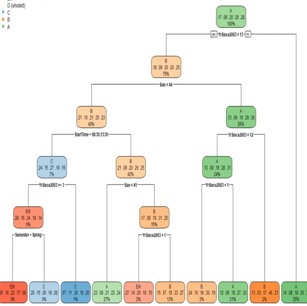
tree is given in figure 5.1.1. Note that the resulting classification tree only considers the inputs ‘YrSince2003’, ‘Size’, ‘StartTime’, and ‘Semester’, whereas all the other inputs did not increase the node purity from the Gini index. Also, it appears that
5.1. Implementing CART in R 34 the probability of receiving a D in each node is never the highest probability.
Figure 5.1.1: CART model for cp=0.001869883 and maxdepth= 5
Each of the colored nodes in figure 5.1.1 contain three pieces of information work-ing from the top of the node to the bottom: the most likely student grade; the probabilities of each grade; and the percentage of the data set that this observation represents, respectively. Denote the terminal nodes R1, R2, . . . , R10 moving from the
proba-5.1. Implementing CART in R 35 bilities of each grade starts with the probability of EW on the left and ends with the probability of A on the right.
Looking at the initial the initial node, the recursive binary splitting to the left, indicating a ‘yes’, is {X|Y earSince2003<13}, and the recursive binary splitting to the right, indicating a ‘no’, is {X|Y rSince2003≥14}.
Looking at the terminal node R9, we observe that this node predicts a B, with a
probability of 46%, which contains 2% of the ‘Grades.testing’ testing set. To reach the terminal node R9, we have to have the years since 2003 be less than 13, the class
size greater than or equal to 45, and the years since 2003 be, more specifically, greater than or equal to 12. This can be summarized as a class with 45 students or more, and there are exactly 12 years since 2003, i.e. the year is 2015. Equivalently, the terminal
R9 can be summarized as
R9 ={X|Y earSince2003 = 12, & Size≥45}.
Consider the same conditions as for POLR and VGLM: a class ‘MAT135’ class in the spring of 2003; with a start time of 08 : 30 am; that meets 4 days a week; and that contains 44 students. Since the classification tree above only uses four inputs we can summarize this as a class with 44 students; a start time of 08 : 30 am; the years since 2003 as zero; and the class in the spring. If we following these rules down the classification tree, we will reach the terminal node R7 which predicts that a student
under these conditions will most likely get the grade B with a 30% probability. Also, the probability of getting an A is 19%, the probability of getting a C is 18%, the probability of getting a D is 10%, and the probability of getting an EW is 24%. This CART model is visually more interesting and easier to interpret, as we do not need to deal with interpreting logit links and cumulative probabilities.
5.2. Prediction and logLoss for CART 36
5.2
Prediction and logLoss for CART
Just as before, we can use the ‘mlogloss’ function to generate the logLoss value of the CART models with a cp of 0.001869883 and a maxdepth of 5. The R code that implements this is found in appendix D. Creating predicted probabilities for each student grade for the same input values as our example, we have the results below.
> p r e d i c t . c a r t [1 ,]
EW D C B A
0 . 2 3 8 8 0 5 9 7 0 . 0 9 7 0 1 4 9 3 0 . 1 7 9 1 0 4 4 8 0 . 2 9 8 5 0 7 4 6 0 . 1 8 6 5 6 7 1 6
Notice that terminal nodeR7 predicted the grade B with a 30% probability. Also, all
the other probabilities are the same as in our example. Finally, we get a logLoss of 1.52279 for cp of 0.001869883 and maxdepth= 5. We see an improvement compared to the data models, as the POLR and VGLM models had a logLoss of 1.541234.
37
Chapter 6
Random Forests Tree Model
A problem associated with classification trees is that they have high variance [8]. In other words, a small change in the data set leads to a large change in the classi-fication tree with different results. Also, the CART model can be defined as a weak learner: where introducing too many predictors to the model will cause inaccuracy, as if the algorithm gets overwhelmed. We will see that the RF model is a technique of combining a large number of weak learners to make a strong learner. The following overview of the random forests model is taken from [8] and [13].
The bootstrap method is used to fix the high variance in the CART model. Ba-sically, bootstrapping averages a set of observations to reduce the variance. So, to reduce variance and increase accuracy one can take several training sets, build a model for each of the training sets, and then average the resulting predictions. Since we do not have access to several training sets, a technique called bagging, or bootstrapped aggregation, can be used.
For bagging, we take our data set, in our case the testing set, and select B, a number of random (bootstrap) samples with replacement, where each bootstrap will be the same size as the original data set. In fact, the number B is the total number of classification trees grown by the random forests model. For the b-th bootstrap we apply the model, obtain the prediction, and average the prediction results. For the RF model, we calculate the classification predictions ˆC1(X0),Cˆ2(X0), . . . ,CˆB(X0) on
38 the classification trees are grown without complexity pruning. This can be done by setting cp = 0 for the CART model, allowing each tree to have high variance and low bias.
Averaging reduces the variability of the low biased classification trees. The aver-aging part of bagging for a classification problem is done by taking a majority vote from each of the predictions ˆCb(X) for some bootstrapb. Majority voting is the
over-all prediction of the most commonly occuring class in the B bootstraps [8]. Bagging is a simplified method to bootstrapping as we take some number n < N, whereN is the number of observations in the data set. A problem that arises with randomized samping is we may get a set of bootstraps that are similar, creating highly correlated trees. If we average correlated classification trees, we do not improve the variance issue. This problem is fixed in the RF model.
Random forests uses bagging and decorrelates the classification trees [8]. Instead of building a classification tree with k inputs under consideration for each node, a subset of predictors, namely mtry, are considered at each node. This avoids a computationally expensive model when building a large number ofBtrees. A common choice is mtry ≈√k. From chapter 2, cross validation determined that the number of input variables to consider at the splitting of each node is two, i.e. mtry = 2. The splitting rule used in the RF model is the Gini index, G from 5.0.1.
The RF model takes into account the strength of each of the inputs. From the CART model, the stronger inputs were ‘StartTime’, ‘Size’, ‘Semester’, and ‘YrSince2003’. For each of the classification trees, the bootstrap sample takes into account the stronger inputs and these are used in the initial node split more frequently. These stronger inputs are the inputs that maximize node purity in the Gini index.
To summarise, the RF model buildsB number classification trees, decorrelates the classification trees by only selectionmtryinputs to split at each node, and implements a majority vote to find the probabilities. Algorithm 6.1 outlines how to build RFs
39 and is based on the work done in [13]. For algorithm 6.1, X are the inputs in the testing set.
Algorithm 6.1 Training, Testing, and Fitting the Random Forests model Training Set (using logLoss):
1. Apply K- fold cross validation to find the number of inputs to split at each node and the number of bootstraps B =num.trees.
Testing Set and Building the Tree (using the Gini index and logLoss): 2. Obtain B bootstraps from the testing set.
Forb = 1,2, . . . , B:
3. Obtain the corresponding classification tree Tb for each bootstrap b using the
CART algorithm 5.1 with cp = 0.
(a) Select a mtry random number of inputs from X.
(b) Select which of the random inputs increase node purity using the Gini index.
(c) Binary split the node using one of the inputs, and stop when there remains only one class left in the node, i.e. min.node.size = 1.
4. Return all the classification trees for each bootsrap b: {Tb}B1.
LetX0 be vector of input values that you want to use to make a prediction:
5. Obtain the classification prediction ˆCb(X0) for each of the b-th random forest
classification tree. Then, ˆ
6.1. Implementing Random Forests in R 40 Here, ‘forest’ refers to the fact that we are growing a large number of classifications trees. A downside to RF is we do not have any equations, such as POLR and VGLM, to use to make predictions on paper. We require a statistical program to make predictions using the RF model. Therefore, bagging improves the prediction accuracy at the expense of interpretability [8]. Note that after a probability distribution is created using ˆCrfB(X0) in step 5, we can test the random forest model against the actual grades obtained from the ‘datatest’ set, use the logLoss equation 2.1.1, and find the final logLoss value of the model.
6.1
Implementing Random Forests in
R
First, the RF model is built with R, then that model is used to make predic-tions. The RF model was built using the Gini index splitting rule, implemented by
splitrule= “gini”; only allowing the classification treesTb to terminate growth when
there is only one class left in a node, implemented bymin.node.size= 1; only allow-ing two random predictors to be considered in splittallow-ing each node, implemented by
mtry = 2; and finally, setting the number of classification trees the RF model will grow as B =num.trees= 1500. It is not feasible to plot all of the 1500 trees, so the
Rprogram stores the model instead. To grow the random forest, we used the ‘ranger’ function in the ‘ranger’ package [23]. The output from the ‘ranger’ function, where the RF is stored in ‘Grades.rf’, is given below.
> p r i n t ( G r a d e s . rf ) R a n g e r r e s u l t C a l l : r a n g e r ( G r a d e ~ S e m e s t e r + S i z e + S t a r t T i m e + Day + C l a s s + Y r S i n c e 2 0 0 3 , d a t a = G r a d e s . testing , m t r y = 2 , s p l i t r u l e = " g i n i " , i m p o r t a n c e = " i m p u r i t y " , min . n o d e . s i z e =1 , num . t r e e s =1500 , p r o b a b i l i t y = TRUE , c l a s s i f i c a t i o n = T R U E )