Air Force Institute of Technology
AFIT Scholar
Theses and Dissertations Student Graduate Works
3-23-2017
An Analysis of Forecasting Methods on Supply
Discrepancy Reporting
Cody S. Freeborn
Follow this and additional works at:https://scholar.afit.edu/etd
Part of theOperations and Supply Chain Management Commons
This Thesis is brought to you for free and open access by the Student Graduate Works at AFIT Scholar. It has been accepted for inclusion in Theses and Dissertations by an authorized administrator of AFIT Scholar. For more information, please [email protected].
Recommended Citation
Freeborn, Cody S., "An Analysis of Forecasting Methods on Supply Discrepancy Reporting" (2017).Theses and Dissertations. 1640. https://scholar.afit.edu/etd/1640
AN ANALYSIS OF FORECASTING METHODS ON SUPPLY DISCREPANCY REPORTING
THESIS MARCH 2017
Cody S. Freeborn, Captain, USAF AFIT-ENS-MS-17-M-130
DEPARTMENT OF THE AIR FORCE AIR UNIVERSITY
AIR FORCE INSTITUTE OF TECHNOLOGY
Wright-Patterson Air Force Base, Ohio DISTRIBUTION STATEMENT A.
The views expressed in this thesis are those of the author and do not reflect the official policy or position of the United States Air Force, Department of Defense, or the United States Government. This material is declared a work of the U.S. Government and is not subject to copyright protection in the United States.
AFIT-ENS-MS-17-M-130
AN ANALYSIS OF FORECASTING METHODS ON SUPPLY DISCREPANCY REPORTING
THESIS
Presented to the Faculty Department of Operational Sciences Graduate School of Engineering and Management
Air Force Institute of Technology Air University
Air Education and Training Command In Partial Fulfillment of the Requirements for the
Degree of Master of Science in Logistics and Supply Chain Management
Cody S. Freeborn, BS Captain, USAF
March 2017
DISTRIBUTION STATEMENT A.
AFIT-ENS-MS-17-M-130
AN ANALYSIS OF FORECASTING METHODS ON SUPPLY DISCREPANCY REPORTING
Cody S. Freeborn, BS Captain, USAF
Committee Membership:
Dr. Michael Kretser
Chair (Primary Research Advisor)
Dr. Alan Johnson Member
iv AFIT-ENS-MS-17-M-130
Abstract
The Department of Defense (DoD) tracks and records all cargo shipments as they move from one location to the next. Inevitably, there are mistakes that are made when dealing with these shipments. Currently the Air Force does not use any forecasting techniques to predict these shipping discrepancies, thus it has no way to prepare for them other than employing remedial measures after errors occur.
The purpose of this research is to study the current Air Force shipping processes, specifically shipping discrepancies, and determine if any trends emerge. By examining historical shipment discrepancy data, a trend analysis was accomplished and from this data a relatively accurate forecast was developed.
In the final analysis, it was concluded that three models most accurately forecasted the behavior of the discrepancy codes studied. These three models can be utilized in determining the root causes of these discrepancy trends. If employed, focused training events should reduce costs to the Air Force through cost avoidance through by circumventing lost time and resources normally expended correcting shipping errors.
v
Acknowledgments
I would like to express my sincere appreciation to my faculty advisor, Capt Michael Kretser, for his guidance and support throughout the course of this thesis effort. The insight and experience was certainly appreciated. I would, also, like to thank my sponsor, Ms. Linda Lowin, from the Air Force Installation and Mission Support Center for both the support and latitude provided to me in this endeavor.
vi Table ofContents Abstract ... iv Acknowledgments...v List of Figures ...x List of Tables ... xi I. Introduction ...1 Purpose ...1 Background ...2 Problem ...3 Justification ...3 Assumptions ...4 Scope ...4 Methodology ...5 Research Objectives ...5 Research Questions ...5 Organization ...6
II. Literature Review ...7
Overview ...7
Air Force Shipment Errors ...7
Forecasting ...13
Shipment Errors ...17
Forecasting to Reduce Shipping Errors ...19
III. Methodology ...23
Overview ...23
Data Collection ...23
Tools ...25
Methodology Used to Address the Research Questions ...25
Time Series Regression...26
vii Trend ...26 Seasonal ...27 Cyclical ...27 Additive...27 Multiplicative ...28 Exponential Smoothing ...28 Simple ...28 Holt’s Trend ...28 Holt-Winters ...29 Box Jenkins ...30
Choosing the Methods ...30
Validity Assumptions...31
Parameters ...31
Sum of Squared Errors ...31
Coefficient of determination ...31
Mean Absolute Percentage Error ...32
Relative Absolute Error ...33
Theil’s U-statistic ...33
Comparison ...34
IV. Results and Analysis ...35
Overview ...35
Forecasting Methods ...35
Practical Application of the Forecasting Techniques ...37
D1 (Documentation Not Received) ...37
D3 (Documentation Incomplete/Improper) ...40
Q11 (Returned PDQR Exhibit Deficiency) ...42
Z3 (Distribution Center Receipt Not Due-In) ...44
P113 (Electrostatic/Electromagnetic Device Preservation Inadequate or Omitted) ...46
P201 (Container Inadequate/Incorrect/Oversized) ...48
viii
P210 (Non-Conformance to Specified Requirements for Packing) ...52
P303 (Labels Omitted or Improperly Affixed) ...54
Final Analysis ...56 V. Discussion ...58 Overview ...58 Current Process ...58 Conclusion ...59 Recommendations ...59 Limitations ...60 Future Research ...60
Appendix A. Naïve Forecast Sample ...61
Appendix B. Simple Linear Regression Sample ...62
Appendix C. Trend Sample...63
Appendix D. Dummy Sample ...64
Appendix E. Trigonometry Sample (1-year cycle) ...65
Appendix F. Trigonometry Sample (2-year cycle) ...66
Appendix G. Trigonometry Sample (3-year cycle) ...67
Appendix H. Trigonometry Sample (4-year cycle) ...68
Appendix I. Autocorrelation Sample (1-year cycle) ...69
Appendix J. Autocorrelation Sample (2-year cycle) ...70
Appendix K. Autocorrelation Sample (3-year cycle) ...71
Appendix L. Autocorrelation Sample (4-year cycle) ...72
Appendix M. Decomposition Multiplicative Sample (12 month) ...73
Appendix N. Decomposition Multiplicative Sample (4 month) ...74
Appendix O. Decomposition Additive Sample (12 month)...75
Appendix P. Simple Exponential Smoothing Sample ...76
Appendix Q. Holt’s Trend Sample ...77
Appendix R. Additive Holt-Winters Sample (4 month) ...78
Appendix S. Additive Holt-Winters Sample (12 month)...79
ix
Appendix U. Multiplicative Holt-Winters Sample (12 month) ...81 Appendix V. Comparison Chart Sample ...82 Bibliography ...83
x
List of Figures
Page
Figure 1. D1 Validity Assumptions ... 38
Figure 2. D1 Forecast ... 39
Figure 3. D3 Validity Assumptions ... 41
Figure 4. D3 Forecast ... 41
Figure 5. Q11 Validity Assumptions ... 43
Figure 6. Q11 Forecast ... 44
Figure 7. Z3 Validity Assumptions ... 45
Figure 8. Z3 Forecast ... 46
Figure 9. P113 Validity Assumptions ... 47
Figure 10. P113 Forecast ... 48
Figure 11. P201 Validity Assumptions ... 49
Figure 12. P201 Forecast ... 50
Figure 13. P206 Validity Assumptions ... 51
Figure 14. P206 Forecast ... 52
Figure 15. P210 Validity Assumptions ... 53
Figure 16. P210 Forecast ... 54
Figure 17. P303 Validity Assumptions ... 55
xi
List of Tables
Page
Table 1. Comparison Chart ... 36
Table 2. D1 Comparison Chart ... 37
Table 3. D3 Comparison Chart ... 40
Table 4. Q11 Comparison Chart ... 42
Table 5. Z3 Comparison Chart... 44
Table 6. P113 Comparison Chart ... 46
Table 7. P201 Comparison Chart ... 48
Table 8. P206 Comparison Chart ... 50
Table 9. P210 Comparison Chart ... 52
AN ANALYSIS OF FORECASTING METHODS ON SUPPLY DISCREPANCY REPORTING
I. Introduction
Purpose
The Department of Defense (DoD) tracks and records all cargo shipments as they move from one location to the next. The information collected is vast and includes details about each item, not only the origin and destination, but also any important details about the shipment. Inevitably, there are mistakes that are made when dealing with these shipments. Shipping errors can be as simple as improper labeling, or can be as disastrous as shipping the wrong item or shipping to the incorrect location. Currently the Air Force does not use any forecasting
techniques to predict these shipping discrepancies, thus it has no way to prepare for them other than employing remedial measures after errors occur. This research will focus on determining whether traditional forecasting techniques are capable of forecasting these shipping discrepancies or if new techniques need to be developed.
The purpose of this research is to study the current Air Force shipping processes, specifically shipping discrepancies, and determine if any trends emerge. By examining historical shipment discrepancy data, a trend analysis was accomplished and from this data a relatively accurate forecast was developed. The ability to forecast the discrepancies that impact the Air Force the most will allow managers to prepare for these errors and eventually be able to prevent or reduce the number of them from happening.
Background
All shipping errors that the DoD observes are recorded as Shipping Discrepancy Reports (SDRs). An SDR is a tool used to report shipping or packaging discrepancies attributable to the responsibility of the shipper, and to provide appropriate responses and resolution, including financial action when appropriate. The purpose of the SDR exchange is to determine the cause of such discrepancies, effect corrective action, and prevent recurrence. All SDRs are tracked and maintained on a web based application called DoD WebSDR. DoD WebSDR is an application that enables SDR transaction exchange, provides a web-based entry method, and provides visibility of SDRs for research and trend analysis via management report/query capability. It is essentially a large database in which all SDRs are maintained. This was the source of all quantitative data used for this research.
The Air Force Installation and Mission Support Center (AFIMSC) Traffic Management section is responsible for the majority of the SDR process. The entire process was originally owned by the Material Management section, but was transferred to the Traffic Management section when the inbound cargo receiving and receipt functions were combined. Material Management still maintains a role however, due to many of the reasons for discrepancies
originating from inventory and stock control issues. Therefore, the combined effort of these two sections will be manifested in the form of a functional project with the goal to reduce overall discrepancies. Because of the large amount of discrepancies that occur each year, Traffic
Management intends to identify specific and controllable discrepancies from an enterprise view. This will enable them to pinpoint which agencies are responsible for these discrepancies and ensure that proper training is conducted in order to reduce future errors.
Problem
Currently the Supply Discrepancy Reporting process is managed and affected by two different offices. Neither of these offices are conducting effective preventative measures to reduce discrepancies, and neither of them are communicating issues well because they are not aware of what issues they have. Due to these reasons, the Air Force has no way to accurately predict when and where discrepancies will occur.
The current SDR database is a cumbersome system that proves difficult to use or to pull valuable information from. The system is designed to provide individual discrepancy
information as well as enterprise level discrepancy trend data. Unfortunately, the system is best used on a case-by-case basis to gain information on specific discrepancies, but is not designed to inform users of any discrepancy trends. Managers do not have an accurate picture of what discrepancies are on an upward trend, downward trend, or which locations are the most common culprits of these mistakes.
AFIMSC is continually working to reduce supply discrepancies, but in order to make progress it needs to pinpoint the root cause of these discrepancies. Currently it is not equipped to make these determinations. This analysis will assist managers in identifying the problem areas and provide AFIMSC a plan of action to correct these mistakes.
Justification
Shipping errors cost the Air Force and the DoD time and money. Currently the Air Force does not have an effective method for tracking these discrepancies to their root causes. If this research can help pinpoint at least some of the origins of these shipping discrepancies it will result in a reduced number of SDRs. Once these causes have been identified, the Air Force will
be able to apply corrective action, not only at problem areas, but at Traffic Management Offices around the world. Implementing a change like this will reduce overall costs and improve shipping efficiency across the Air Force.
Assumptions
This research is limited by the available quantitative data, which is accessed through the WebSDR database. This research assumes that the data pulled from WebSDR has been recorded correctly and accurately represents the SDR historical record. WebSDR is maintained under the Defense Logistics Management Standards, which provides a base of business rules, data
standards, and electronic business objects designed to meet DoD’s requirements for total
logistics support. This research assumes that under the purview of DLMS, WebSDR records are maintained correctly.
Scope
This study focused on the total number of Air Force shipment discrepancies for specific discrepancy codes. The decision to exclude location information of each discrepancy was conducted to allow for the researcher to focus on one specific variable; the discrepancy code itself. In order to complete the study in a timely manner two groups of SDRs were analyzed. After studying the most common discrepancies over the last three years, the top five most
common discrepancy codes were selected for the study. At the request of the AFIMSC, a similar selection process was completed for the top five most common packaging discrepancy codes. One of the top packaging discrepancy codes was also one of the top overall discrepancy codes. These two groups (9 total codes) are the focus of this research.
Methodology
Data for this research was collected from the WebSDR database. Data for each of the 9 discrepancy codes were collected in monthly increments and include a five year historical record. Once these time series data were compiled, a thorough forecasting analysis was conducted. The statistical tools used to conduct this analysis were MS Excel and JMP.
Research Objectives
The primary objective of this research is to identify the most costly and most common SDRs the Air Force currently deals with and create forecasting models to assist Traffic Managers in predicting and reducing SDRs.
Also, as a result of this research, many different forecasting models were tested on this data. Based on the results of these tests, this study will recommend specific forecasting techniques for Traffic Managers to use in the future.
Research Questions
In order to address the objective listed above, the following questions were established and will be answered during the course of this research:
• How can the Air Force better forecast SDRs?
• How can the Air Force assess the validity of these forecasts?
Organization
Chapter I provides an introduction to the topic of the study as well as the necessary background information the reader will need to establish a foundation which the following chapters will build upon. This chapter also provides an overview of the problem, methodology, scope, and research objectives/questions.
Chapter II gives a literature review on shipping errors in the Air Force and how large their impact can be. Also included here is an analysis of the various forecasting concepts which are used in this study.
Chapter III details the specific methods used in this study to collect data, conduct a statistical analysis, and the parameters chosen to test the validity of these results.
Chapter IV reviews the results of the analysis that was detailed in Chapter III. This chapter aims to answer the research questions presented and to determine the validity of the tests themselves.
Chapter V discusses the results of the study and presents the conclusions and recommendations for further research in this field.
II. Literature Review
Overview
This chapter discusses the history the Air Force has with shipping errors and how these errors have a lasting impact on the military. An introduction to forecasting techniques and concepts is provided as well. Literature on shipping discrepancies is explored and the benefits of combining forecasting with traffic management is discussed.
Air Force Shipment Errors
Shipping errors can have large implications depending on what is being shipped and which parties are involved. Shipping the wrong item or shipping to the wrong location can be disastrous for the Air Force and the DoD. A mistake like this could result in the loss of classified weapons or material to the enemies of the United States, which is why conducting proper
shipment precautions is extremely important. In the mid 2000’s, the USAF committed two very serious mistakes that involved the handling and shipment of nuclear weapons.
The first incident took place on August 31, 2007, as “a U.S. Air Force B-52 plane with the call sign “Doom 99” took off from Minot AFB, North Dakota, inadvertently loaded with six Advanced Cruise Missiles loaded with nuclear warheads and flew to Barksdale AFB, Louisiana. After landing, “Doom 99” sat on the tarmac at Barksdale unguarded for nine hours before the nuclear weapons were discovered”(Spencer et al., 2012). The decision to move these cruise missiles from Minot AFB to Barksdale AFB was part of an Air Force re-positioning program. Since these two bases are the only bomber wings that currently support the B-52 airframe, flights
between these two locations are fairly regular for the bomber squadrons. Therefore, if munitions need to be moved from one base to the other, the Air Force can save money by loading the munitions in the bomb bay of an aircraft that is departing to the other base rather than requiring a cargo aircraft to complete the shipment. This is an efficient way to transport cargo and relocate aircraft in the same movement, unfortunately several mistakes were made during the shipment of these weapons (Plante, 2010; Spencer et al., 2012).
There were 12 total missiles that were originally scheduled to ship from Minot AFB to Barksdale AFB. These missiles were intended to be loaded with nonnuclear Tactical Ferry Payloads (TFPs) instead of live payloads, such as nuclear warheads. The 5th Munitions
Squadron was in charge of preparing the missiles for transport and they began by loading all of the missiles on two separate missile pylons, each holding 6 missiles. All of these missiles were meant to be loaded with TFPs before departure, but before departure the munitions control section changed which missiles were to be shipped, but did not communicate this to the nuclear weapons maintenance shop, who were responsible for preparing the TFPs. Because of this miscommunication, 6 missiles were prepared correctly and the other 6 were carrying nuclear warheads (Spencer et al., 2012).
At the time there was a shortage of storage space for these missiles, which meant that both nuclear and nonnuclear cruise missiles were often stored in the same location. Since the only way to identify the difference between a nuclear and a nonnuclear missile is by looking through a small observation window to check for the appropriate markings, proper protocol is to mark the missiles with a placard. Only one missile pylon had been marked with a placard stating “Ready for Tac Ferry”. The other pylon had no placard, so the handling crew assumed that it
was the same as the other pylon rather than following the missile safe status check to ensure that both pylons were loaded with TFPs (Spencer et al., 2012).
When the missiles were brought to the aircraft, both the Radar Navigator and the Navigator are responsible for verifying the status of the missiles during preflight inspections of the aircraft when dealing with nuclear weapons. Unfortunately, only the Radar Navigator performed the preflight inspections. Also, when conducting the inspection, the Radar Navigator only checked one of the two pylons, which happened to be the nonnuclear pylon. He then made the assumption that the other pylon was correct and cut the preflight inspection short. “Doom 99” then made the trip from Minot to Barksdale and sat on the tarmac unguarded for 9 hours before the Barksdale handling crew came to transport the missiles to the storage facility. This crew conducted the inspection correctly and discovered the pylon of nuclear missiles and immediately alerted their leadership (Spencer et al., 2012).
Several specific errors in procedure had to take place to allow this mishap to occur. The first mistake was the not correctly labeling the pylon trailers. This was an individual mistake, but one that was probably influenced by the decision to store nuclear and nonnuclear missiles in the same location. The second error was a communication breakdown between the munitions personnel and the maintenance personnel. This was a scheduling error and resulted in an
alternate set of missiles to be used for the transport (the missiles loaded with nuclear warheads). The third and fourth mistakes came when the munitions personnel did not oversee the movement of the weapons and the handling crew did not follow the checklist to ensure that the weapons were nonnuclear. The fifth error occurred on the flight line when the aircraft crew chief signed off on the weapons without confirming their status. The final error that took place was when the radar navigator on the aircraft did not follow his checklist and only inspected one of the two
pylons. These seven errors explain how these nuclear weapons were mistakenly shipped to Barksdale AFB (Norris et al., 2016; Spencer et al., 2012).
After the nuclear missile shipment incident occurred, the Air Force began tightening down on its nuclear program. Unfortunately, this is when it was revealed that Taiwan had
received classified sections used on the Minuteman III intercontinental ballistic missile instead of helicopter batteries as it had ordered from the United States (Spencer et al., 2012).
The Air Force uses a supply system called Readiness Based Leveling to conduct service-wide adjustments to ensure that all locations have the correct inventory levels of items in their warehouses. This system in used semi-annually and in February of 2005, this system identified a requirement for 11 forward sections of the MK-12 reentry vehicles used on the Minuteman III intercontinental ballistic missiles (ICBM) at F.E. Warren AFB, Wyoming. The system showed that there was currently one of these forward sections at F.E. Warren AFB, so an automatic transaction to ship 10 units was completed. When the forward sections were delivered they were properly received and stored under a controlled-item status (Spencer et al., 2012).
After this shipment was completed, an inexperienced Air Force Item Manager at the 526th
ICBM Systems Group at Hill AFB, Utah determined that F.E. Warren actually had too many MK-12 forward sections and directed the base to ship four of these forward sections to the Defense Logistics Agency (DLA) warehouse at Hill, AFB. After receiving this guidance, the F.E. Warren Traffic Management Office (TMO) packed the forward sections and prepared them for shipment. The F.E. Warren TMO placed the shipping documents inside the shipping
container, but did not properly mark the exterior with the stock number as directed by the packaging instructions. Classified items like these are shipped with all documentation packed inside the container. Protocol requires the recipient to open the container, inspect the documents
and ensure that the contents of the container match the documents, sign a receipt and then send that receipt to the shipper. This process is used to ensure that the correct items are shipped and that the recipient verifies the delivery of the correct items (Spencer et al., 2012).
Unfortunately, the F.E. Warren TMO did not mark the outside of the shipping container which contained hazardous and classified cargo. When the shipping container arrived at the Hill AFB warehouse, the personnel did not open it, review its contents, sign a receipt, or return a receipt to F.E. Warren. F.E. Warren didn’t even follow-up on the missing receipt as is required. Since the personnel at Hill AFB did not even open the shipping container they assumed that it was unclassified, nonhazardous material, so they stored it in an unclassified warehouse instead of the classified storage area. At a later date, DLA warehouse personnel tried to scan the barcode on the unopened shipping container in order to identify the contents. The scan was unsuccessful, so the warehouse personnel decided to use the hazard classification for the nomenclature and they arbitrarily selected a number that was for a helicopter battery. They marked the shipping container with this new identification and stored it in the warehouse labeled as helicopter batteries (Spencer et al., 2012).
The Air Force participates in the Foreign Military Sales Program where international partners have the opportunity to purchase certain items from the United States Government. This usually involves the sale of retired aircraft or aircraft parts that the United States no longer has a use for, but other countries may still use (Marion, 2013).
In 2005, the government of Taiwan requested 135 helicopter batteries through the use of the Foreign Military Sales Program. In 2006, the DLA warehouse at Hill AFB shipped the mismarked MK-12 forward sections as helicopter batteries. Taiwan identified the error in January of 2007 and an immediate investigation ensued (Spencer et al., 2012).
Similar to the shipment of the nuclear warheads, several different mistakes resulted in the unauthorized movement of these MK-12 forward sections. The first mistake was the incorrect marking of the shipping container by the F.E. Warren personnel. The second mistake occurred when upon arrival at Hill AFB the container was never opened and inspected. The third mistake was when the barcode could not be properly scanned and the warehouse personnel assumed what was inside the container rather than opening the container to properly identify its contents. The fourth mistake was that the personnel at F.E. Warren never followed up after never receiving the shipment receipt from Hill AFB. The final mistake was that the error was only confirmed by the United States government after several requests by the Taiwanese government to correct the shipment (Spencer et al., 2012).
These two incidents demonstrate the importance of following the correct shipment
procedures for all DoD shipments. Mistakes like these can and will happen if precautions are not taken. Proper training and instruction for Traffic Management Offices, warehouse personnel, handling crews, and anyone who deals with shipments in any capacity is paramount to ensure accurate and timely delivery of supplies. Training will reduce shipping errors, but will not fully eliminate them. As long as the system is operated by humans, there will always be shipping errors. So if managers cannot eliminate these shipment errors, they can plan for them and work around them. If a manager has the ability to forecast and predict when and where errors will occur, they will be able to focus their efforts in that area in order to reduce the number of errors. If managers can identify a pattern in these errors this may help them identify the root cause of these mistakes and assist them in eliminating these faults all together.
Forecasting
Forecasting is an important tool that can be used to help predict future events. Though it is not quite an exact science, it depends on a set of statistical tools and techniques that are used in conjunction with human judgement and intuition. Hyndman and Athanasopoulos describe it as predicting the future as accurately as possible, given all of the information available, including historical data and knowledge of any future events that might impact the forecasts. Forecasting techniques can be applied in a wide range of fields including operations management, marketing, finance, risk management, economics, industry, and others. Although, certain events can be more accurately forecasted than others. For instance, the earth’s weather patterns are predictable and can be forecasted with reasonable accuracy. In contrast, the winning numbers for the next Powerball drawing does not follow any sort of pattern and cannot be accurately predicted (Hyndman & Athanasopoulos, 2014).
In order to correctly predict an event there are certain factors that must be met. First, the researcher must understand all of the factors that contribute to the event. If there are certain variables that are not accounted for, the prediction will be inaccurate. Second, there needs to be an adequate amount of historical data. If there is little history to draw from, the forecast will rest heavily on human judgement rather than statistics based techniques. Third, the researcher must know whether the forecasts can affect the phenomenon that is being forecasted. This type of bias often occurs in the stock market. When sources advise that a stock will rise or fall, investors will buy or sell accordingly. This will cause the stock price to rise or fall and the forecast has
effectively influenced the stock price (Hyndman & Athanasopoulos, 2014).
These factors help to determine whether or not an accurate forecast can be achieved. If one or more of these factors are not taken into account, the accuracy of the prediction will suffer.
Even when data are abundant, we may not fully understand all of the contributing variables, which will reduce the accuracy of the forecast. Each situation will vary with what information is available, what patterns can be observed, and what historical timeline is accessible. Sometimes there won’t be any historical data at all, such as forecasting sales for a new product. These are all factors that must be taken into account (Hyndman & Athanasopoulos, 2014).
Forecasting is often used in business to help managers make decisions about inventory, scheduling orders, and aid in strategic planning. In order to effectively forecast, managers must establish goals which they want to achieve and develop a plan of how to achieve these goals. Goals should be developed with forecasts in mind to ensure that they are realistic. Likewise, plans should be developed in response to forecasts and goals. They will determine what actions need to be taken to meet these goals (Armstrong, 2001b).
Most organizations develop forecasts of different lengths to help achieve their goals. Short-term forecasts focus on the scheduling of production, inventory, employees, transportation, and distribution. These are the daily demand forecasts that help plant and warehouse managers stay on top of fluctuations. Medium-term forecasts are used to determine requirements in the near future. This includes hiring of personnel, ordering and shipment of raw materials, and purchasing of equipment. From a production perspective, this type of planning is done not only at the plant manager level, but also at the branch manager level. Finally, long-term forecasts are used in strategic planning for the firm as a whole. These forecasts take into account changes in the market, economic trends, possible opportunities for expansion, and even environmental factors (Armstrong, 2001b).
It is important for firms to develop multiple approaches to dealing with events. The combination of these different forecasts allows the firm to mold their plans to not only be
realistic, but also be accurate. The short-term models will have the most accuracy, but the others will provide insight on trends that the firm must be aware of (Armstrong, 2001a).
There are two different types of forecasting methods; qualitative and quantitative. Qualitative methods are based on human judgement, expert opinions and past experience. This type of forecasting is usually conducted when there is little to no data available, or if the
available data does not assist in developing an accurate forecast. Quantitative forecasting can be used when there is applicable data available and there is reason to believe that there is somewhat of a pattern in the historical data that will continue. There are many different types of
quantitative methods to choose from, all with differing specific purposes. Most either use time series data, which is collected at specific intervals over time, or cross-sectional data, which is collected at a single point in time. Although, before deciding on which method and model to use there are certain steps that must be taken (Hyndman & Athanasopoulos, 2014).
Forecasting usually involves five basic steps; defining the problem, gathering
information, initial analysis, choosing and fitting models, using and evaluating a forecasting model. To begin, managers must identify the problem which they want to solve. This can be difficult because often the symptoms of a problem are observable, but the root cause remains undefined. Once the problem is correctly defined, managers will now have an understanding of the ways in which forecasts will be used, who needs them, and how they will benefit the
organization (Armstrong, 2001b).
Gathering information is a crucial step which will help determine how accurate the forecast may be. Access to good, usable data allows researchers to develop extremely accurate predictions. Unfortunately, data are not always available. There may be times where no data were collected, or the particular variable that is needed is not available, or the data may not exist
at all. There are two types of data; statistical and judgmental. While both are useful, it is important to understand when to use each and how they work together. With quality data available, statistical models will provide accurate forecasts. However, there will not always be enough historical data to fit a good statistical model. This is when human judgment may be needed to make the best predictions. But what tends to happen the most is a combination of the two. Organizations will collect statistical data and conduct an analysis. This analysis will then be reported to the leadership of the organization, who will then use this information and their accumulated experience to make a decision (Hyndman & Athanasopoulos, 2014).
Once the data is collected an initial analysis can be conducted. The first step a researcher will likely take is to look at the data in different ways. They may graph it to get a visual
representation. They will look for different trends or outliers. They will look for visible patterns or seasonality. They will also look for relationships to other variables that may be influencing the data (Bowerman, O’Connell, & Koehler, 2005).
Next the researcher will test different models and choose the best fit for the forecasted data. This will depend heavily on the available data, any relationships between the data and explanatory variables, and how the forecast will be used. Each model has a different set of assumptions that it uses to make predictions and by testing a few, some will prove more accurate than others (Bowerman et al., 2005).
Once the best model has been determined, it will then be used to make more forecasts. The model will have an associated confidence interval, but the true accuracy of the model will not be determined until the data for the forecast period becomes available. The organization can then reassess the model accuracy and ensure that it remains the best choice (Bowerman et al., 2005).
Both qualitative and quantitative forecasting methods exist. Qualitative forecasting uses human judgement and is very common in practice. There are many instances when judgmental forecasting is the only option due to a lack of historical data, or the data will not become available until later, but a decision must be made now. Qualitative forecasting can also be applied after statistical forecasts are generated. Managers will use the statistical findings and then use their subject matter experience to make a decision. Other times both statistical and judgmental forecasting are accomplished separately and then compared and combined. The accuracy of qualitative forecasting is higher when the forecaster has a high level of experience and knowledge in the field of study and when the forecaster is provided with current information. Obviously experience is important, but judgmental forecasting needs to adjust to changes in information and events as they take place. Although, in most cases, when data are available, this will be the starting point. When quantitative data are available, statistical forecasting will
usually be preferred over judgmental forecasting (Hyndman & Athanasopoulos, 2014). Quantitative forecasts can range from being as simple as a linear model of time series data to being as complex as an exponential smoothing model. Different types of data will require different techniques to make accurate forecasts. A simple linear model will not be able to account for seasonality in the data. Other, more complex models may require unnecessary work for data that follows a simple trend line. The researcher must use good judgment and test multiple models in order to find the best one (Bowerman et al., 2005).
Shipment Errors
This study deals with Air Force shipment errors and investigates the trends that can be identified in the hope to reduce and prevent them from taking place. In 2015 a similar study was
conducted on fulfillment errors at the distribution center of a major retailer (the name of the retailer was not disclosed to protect anonymity). The retailer is a 700-store retailer of apparel, electronics, and housewares (60% of its sales), as well as food items (40% of its sales). But even a large retailer such as this is burdened with shipping a distribution difficulties. The study found that 7% of all of the retailer purchase orders experience a fulfillment error. The most common types of errors include quantity shortages, ticket errors, and inaccurate advanced ship notices, a large majority of these are preventable and correctable at the distribution center level. The study estimated that these errors imposed a cost between 1% and 4% of the distribution center’s operating budget. This percentage is low, but the cost of these errors is substantial and reducing them would be a tremendous benefit to the retailer. (Craig, Dehoratius, Jiang, & Klabjan, 2014)
These types of errors are affecting the container shipping industry as well. One of the biggest challenges for sea lift container shippers is maintaining a high rate of accurate invoices. Pressure to cut costs and reduce rates resulted in a reduction in carrier invoice accuracy as the amount of back-room staff decline. This shifts the burden of ensuring invoice accuracy onto the shippers. The shippers must now spend more time to inspect invoices and ensure that they correctly list what is in each container and where each container must go. Despite these efforts by the shippers it is estimated that over 15% of all ocean carrier invoices contain errors. The cost of these errors range from $50,000 to $150,000 per year for each individual shipper (Morley, 2016).
The trend that has led to this mismanagement of the shipping process is attributed not only to the pressure to reduce cost, but also the growing need to send out invoices quickly. In recent years the shipping rates have been unpredictable. This has influenced carriers and 3PLs to shift their focus from ensuring accurate invoices to getting shipments out quickly. The mistakes
are usually a combination of computer and human error, which ultimately would be reduced by more robust training (Morley, 2016).
This same pressure to get shipments delivered quickly is also experienced in the Air Force. Often there is a compromise in precision in order to get an item shipped on time. Air Force Transportation Officers are well trained and their teams operate at a high level, but there are instances when the “mission” requires these personnel to cut corners a bit to get a shipment out on time.
The Air Force is experiencing a deficit in personnel, which also affects the level of accuracy of these shipments. Most Air Force personnel currently have multiple responsibilities, which results in personnel spreading their focus between different tasks. A reduction in
manpower increases the likelihood of these overworked individuals making a mistake or cutting corners.
Forecasting to Reduce Shipping Errors
Forecasting techniques are widely used among commercial organizations for many different areas. These techniques can be used to help determine customer demand, individual item sales, raw material usage, and even production plant throughput. In fact, forecasting plays such an important role in supply chain management that much of the success an organization experiences can be attributed to accurate forecasting. Alternatively, poor forecasting can prove to be disastrous for organizations. This fact stresses the importance of ensuring that the correct forecasting techniques are used for the right situations.
Managers are always working to optimize their supply chains from raw material collection, to the manufacturing and distribution centers, all the way to the customer.
Forecasting is a tool that is used to improve this process. When management applies forecasting techniques it is usually done on an enterprise level, but this may not always be the best approach. For organizations to have the most accurate information they must conduct forecasts at different levels of the process. There are three different approaches to forecasting that are currently used in commercial ERPs; aggregate, profile, and microforecasting (Arminger, 2003).
Aggregate forecasting takes a broad approach and observes the organization as a whole. It uses inventory information and reduces complexity by ignoring the interactions between parts of the supply chain, but rather looks at the supply chain as a whole. By doing this, managers are able to create a single forecast for each item across the entire supply chain. The issue with a forecast designed like this is that the forecast never studies any specific item or functional area. This means that managers will not be able to determine the individual needs of functional areas along the supply chain, or the reasons why inventory fluctuations are taking place. This
technique is best used to observe general trends, but should not be used to answer specific questions about individual items or supply chain sections (Arminger, 2003).
Profile forecasting observe the throughput of individual functional areas and individual items as they pass through these areas. This technique is characterized by its ability to apply seasonality to the forecast. Since the scope has narrowed down to the functional area level, historical trends about each particular section can be studied and if patterns emerge this can be used to predict future levels. Unfortunately, in large organizations that have multiple production plants there may be multiple variations of the same functional area. This will add variability to the forecast because there may be different issues that are dealt with at each location (Arminger, 2003).
Microforecasting creates a single forecast for each individual item as it passes through each functional area and the supply chain as a whole. The specificity of this forecast allows for trend and seasonality from historical data to be utilized. This technique provides an accurate forecast due to the fact that no information has been combined and each item and section is observed separately. Because of this, managers are provided with up to date and accurate forecast data for each item passing through the supply chain. Though this method is very
beneficial, it can prove to be difficult to maintain. It requires constant database updates to ensure forecasts are current. If this is to be done by employees it will reduce productivity in other areas. The best solution is to automate the process if possible (Arminger, 2003).
These techniques are not solely applicable to products passing through a supply chain, but can also be applied to the errors within that supply chain. Just like the products themselves, the errors that they manifest can be observable, recordable, and predictable. This means that managers have the ability to apply forecasting techniques when studying these errors. When using each of the previously mentioned forecasting methods, managers will obtain information at different levels of the supply chain. If a manager conducted an aggregate forecast on shipping errors it would produce a broad forecast that showed the total number of errors across the entire company. This is a good place to start and can be used as a benchmark for future improvements, but a more detailed approach will be necessary to begin making corrections.
The profile method will help identify the specific offices that are producing the most shipping errors. This will allow management to focus their efforts on the areas that require improvement. But this method does not demonstrate why the errors are happening in the first place, it only gives the manager an idea of where they are coming from. In order for leadership to make significant progress on reducing these errors they will need to conduct a microforecast
of each item or each discrepancy type. This will provide valuable information on what specifically is being shipped incorrectly and what specifically is being done incorrectly. The combination of these three techniques gives management an overview of all shipping errors within the organization, a list of the offices at fault, and a list of items and discrepancy types that are most common with these mistakes. Having this information allows leadership to make specific corrections to these critical areas efficiently and effectively.
III. Methodology
Overview
This chapter provides details on the data used in the study, how the data was collected and compiled, and also the methodology used to analyze the data.
Data Collection
In order to conduct a proper analysis of a problem, the first and most important step is to have good, usable data. If data are not available, or not complete, the results of the analysis will be weak due to this deficiency. Due to this fact, special care was taken to accurately record data from a DoD web database to ensure the utmost precision.
The data used for this study were pulled from a Defense Logistics Agency (DLA)
Transaction Services web database call “WebSDR” or Web Supply Discrepancy Reporting. This database tracks all shipment discrepancies recorded by every branch of service in the DoD. The amount of information stored in the website is vast, ranging from individual discrepancy details to numbers of discrepancies per time period and location. Data is stored as far back as 2006, which gives researchers an abundant amount of data history to use for analysis.
Since the database contains a large amount of information, the scope of the research needed to be narrowed down. As stated above there are many different types of information available to observe, but to best serve this study, specific supply discrepancy code totals were recorded in monthly increments.
This meant focusing on a small number of specific variables (discrepancy codes). In order to determine which discrepancy codes to study, historical data were pulled for the past three years. The top five most common discrepancies from this time period were used for the study. These discrepancies are Documentation Not Received, Documentation
Incomplete/Improper, Returned PDQR Exhibit Deficiency, Distribution Center Receipt Not Due-In, and Electrostatic/Electromagnetic Device Preservation Inadequate or Omitted which are denoted by D1, D3, Q11, Z3, and P113 respectively. In addition to these discrepancies, the Air Force Installation Mission Support Center requested a focus on discrepancies that specifically pertained to packaging errors. Thus, a similar effort was conducted where the top five most common packaging discrepancies recorded over the last three years were selected to be studied. These discrepancies are Electrostatic/Electromagnetic Device Preservation Inadequate or
Omitted, Container Inadequate/Incorrect/Oversized, Level of Protection Excessive or
Inadequate, Non-Conformance to Specified Requirements for Packing, and Labels Omitted or Improperly Affixed which are denoted by P113, P201, P206, P210, and P303 respectively. All of these discrepancies totaled to 9 because one of the overall top discrepancies was also a top packaging discrepancy code.
Once all of the discrepancy codes were selected, the data collection could begin. Historical data were pulled for monthly increments. From these data pulls the total number of discrepancies and total cost of the discrepancies were recorded per discrepancy code. Data were collected in this fashion until 5 years of data were collected for each discrepancy code.
Tools
The statistical tools used to collect and analyze the data in this study were MS Excel and SAS’s JMP. These are both widely used statistical computing software that are commonly used in forecast analysis.
Methodology Used to Address the Research Questions
This section describes the methods and procedures used to address the formulated research questions.
In order to narrow the scope of this research and determine the most important variables to study, the data collection process described above was conducted. These five discrepancies proved to be the most costly to the Air Force and they, in addition to the requested codes by AFIMSC, will be the focus of this research.
1. How can the Air Force better forecast SDRs?
Forecasting is important for warehousing and supply chain management, but it is not usually used to project errors in the supply chain. To conduct this analysis, an array of different forecasting methods were implemented. The following is a listing and description of the
Time Series Regression
Time series regression is a forecasting method that uses historical data in order to make predictions. A simple regression model uses data and fits a straight line to it. This model is defined by the following equation:
𝑌𝑌= β0+ β1𝑋𝑋+ 𝜀𝜀 (1)
In this equation the Y represents the dependent variable and X represents the independent variables. β0 and β1 represent the intercept and slope of the line respectively. β0 determines the
predicted value of Y when X = 0. Since the data does not fall in a straight line, each observed data point contains random “error”, ε. This does not imply a mistake, but rather a deviation from the linear model.
Decomposition
When time series data does not follow a simple linear model it may exhibit many
different patterns. Depending on the different type of pattern that the data follows, there may be a particular model that will best match that pattern. Decomposition considers some of these patterns and methods to extract the associated components from a time series. For this research two decomposition methods were used; multiplicative and additive. These methods each have three components: trend, seasonal, and cyclical. The following is a description of each
component and how they affect the behavior of the time series.
Trend
Time series follow a trend when there is a long-term increase or decrease in the data. This trend does not necessarily need to be linear, but must be generally positive or negative.
When the pattern of data changes from positive to negative, or vice versa, it is considered to be “changing direction”.
Seasonal
A seasonal time series pattern is determined by seasonal factors, such as day of the week, monthly, or season. Certain products follow a seasonal demand pattern, for example flower sales spike around Valentine’s Day and Mother’s Day. Flower companies will typically sell more flowers in the weeks prior to these holidays than they do during other times of the year.
Cyclical
Data follow a cyclical model when there is a pattern that that is not a simple trend, but also does not fall within a fixed period. This data pattern has peaks and troughs, but they are not associated with a time of year or a seasonality component. Usually these patterns are over two years long.
Additive
The additive model is expressed as the following formula:
Yt= Tt+ St+ Et
(2)
Yt represents the data at period t, St is the seasonal component, Tt is the trend-cycle component, and Et is the remainder (error) component at period t. This model is most appropriate if the magnitude of the seasonal fluctuations does not vary with the level of the time series.
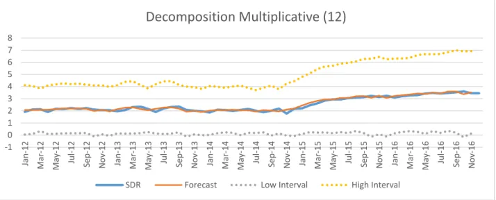
Multiplicative
The multiplicative model is expressed as the following formula:
Yt = Tt × St × Et (3)
The multiplicative model uses the same components as the additive model above. It is most appropriate when the variation in the seasonal pattern is proportional to the level of the time series.
Exponential Smoothing
Exponential smoothing is a type of forecasting model that uses weighted averages of historical data, with the weights decaying exponentially as the observations get older. Essentially, the more recent observations will be weighted higher when making predictions.
Simple
Simple exponential smoothing is most accurate for data that has neither a trend nor seasonal pattern, but does change over time. The equation of the simple exponential smoothing method is as follows:
𝑙𝑙𝑇𝑇 = 𝛼𝛼𝛼𝛼𝑇𝑇 + (1− 𝛼𝛼)𝑙𝑙𝑇𝑇−1 (4)
The current prediction is represented by lT,the smoothing constant is α, the current
observation is
y
T, and the previous prediction is represented by lT – 1.Holt’s Trend
The Holt linear trend method was created to forecast time series that follows some sort of a trend. This method introduces a term into the equation to determine the effect of this variable on the trend. The equation for the Holt trend is shown in Equation 5:
𝑙𝑙𝑇𝑇 =𝛼𝛼𝛼𝛼𝑇𝑇+ (1− 𝛼𝛼)[𝑙𝑙𝑇𝑇−1+𝑏𝑏𝑇𝑇−1] (5)
The components of the Holt’s Trend model are as follows; the current prediction is lT, the
current growth prediction is bT, the smoothing constant is α, the smoothing growth constant is y,
the last observation is
y
T, the previous prediction is lT-1, and the previous growth prediction is bT -1. The initial l0 is the intercept of the regression on the first half of the data, and the initial b0 isthe slope of the regression on the first half of the data.
Holt-Winters
The Holt’s trend method can be modified to forecast data with both trend and seasonal components. These different two data components have two different specific models. The Additive Holt-Winter method is used to forecast constant seasonal variation and the
Multiplicative Holt-Winter Method is used to forecast increasing seasonal variation data sets. The Holt-Winter method equations are as follows:
Additive Holt-Winters:
Yt = (β0+ β1t) + SNt + εt (6)
Multiplicative Holt-Winters:
Yt= (β0+ β1t) x SNt x IRt (7)
In regards to the components of the above Holt-Winters models, the value of the time series in period t is represented by Yt, (β0+ β1t) is the trend component, SNtis the seasonal
component for time period t, IRt is the irregular component in time period t, and εt is the error
Box Jenkins
The Box-Jenkins method refers to the autoregressive moving average (ARMA)
forecasting model. This model’s intended use is to describe the autocorrelations in the data. But before this can be done there are certain requirements that need to be met to ensure an accurate forecast. First, it must be determined whether the data is stationary or seasonal in any way. A stationary data set is one whose properties do not depend on the time at which the series is observed. Essentially, what this means is that to use the Box Jenkins model the data must not have a trend or seasonality. This is best observed using Time Series Diagnostics in JMP. The Sample Autocorrelation Function (SAC) and Sample Partial Autocorrelation Function (SPAC) will exhibit certain behaviors that the researcher will be able to identify as either stationary or nonstationary. When the SAC dies down slowly the data is nonstationary, but when the SAC dies down quickly the data is stationary.
Differencing is a tool that can be used to make a time series stationary. It computes the differences between consecutive observations. This is known as an ARIMA model, adding an “I” for “Integrated”.
Choosing the Methods
Each one of the forecasting techniques listed above were implemented for each of the nine variables in the study. The next step in the process was to determine which method performed the best for each of the individual variables. Five different parameters (discussed in the following section) were chosen to judge the accuracy of each forecast. For each variable tested a table was created that displayed each model and their corresponding parameter results. This table was used to determine the best forecasting technique for each variable.
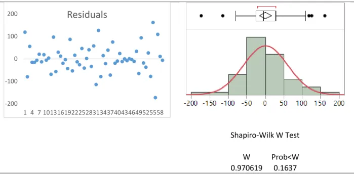
Validity Assumptions
Once the different forecasting models were created it was crucial to determine whether or not they could be used in the study. This means that the model must meet all of the validity requirements, including normality, independence, and constant variance.
2. How can the Air Force assess the validity of these forecasts?
In order to measure the results of these tests, five different parameters were used to compare them: the Sum of Squared Errors (SSE), the coefficient of determination (R2), the Mean
Absolute Percentage Error (MAPE), the Relative Absolute Error (RAE), and the Theil’s U-statistic (Theil’s U). The following are descriptions of the parameters used.
Parameters
Sum of Squared Errors
The sum of squared errors (SSE) is calculated by squaring each error term and summing them. This is a good tool to compare between different tests. The model with the lowest SSE contains the lowest amount of error. The formula is as follows:
𝑆𝑆𝑆𝑆𝑆𝑆 =�(𝛼𝛼𝑖𝑖− 𝛼𝛼�𝑙𝑙)2 (8)
Coefficient of determination
The coefficient of determination (R2) is a figure that represents the accuracy of a forecast,
specifically how well the data fit the statistical model being used. The value of R2 should fall
between 0 and 1, which allows the researcher an easy tool to compare with other models. A score of 0 means that the model does not fit the data at all, while a score of 1 means that the
model is a perfect fit for the data. The coefficient of determination is achieved by dividing the explained variation in data by the total variation.
The formula for explained variation is as follows:
Explained Variation = �(𝛼𝛼�𝑖𝑖− 𝛼𝛼�)2 (9)
The formula for total variation is as follows:
Total Variation =�(𝛼𝛼𝑖𝑖− 𝛼𝛼�)2 (10)
The coefficient of determination (R2) is calculated by dividing the explained variation by the
total variation.
R2 = ∑(𝑦𝑦�𝑖𝑖− 𝑦𝑦�)2
∑(𝑦𝑦𝑖𝑖−𝑦𝑦�)2
(11)
Mean Absolute Percentage Error
The Mean Absolute Percentage Error (MAPE) is a tool that provides a value for the percentage of error in a forecasting model. The higher the value of the MAPE, the more inaccurate the forecast is, and vice versa. Therefore, low MAPE scores are best.
MAPE = �1
n∑
|Actual−Forecast|
Relative Absolute Error
The Relative Absolute Error (RAE) is a tool that is used to compare the accuracy of a model against the accuracy of a naïve forecast (which simply uses the value from each previous period as the forecast). RAE is calculated by dividing the forecast error percentage (MAPE) of the model by the forecast error of the naïve model. The value provided can give the researcher a great deal of information. Obviously a low value is preferable, as the lower the value is the less errors exist in the model. But also what this metric shows the researcher is how the model compares to a very primitive model where the forecast for the next period is simply the number of the current period. If the value is below 1 then the model is better than the naïve model. If the value equals 1 then there is no difference in accuracy between the models. And if the value is greater than 1 the naïve model is actually more accurate than the current model being tested.
The formula for RAE is listed below:
𝑅𝑅𝑅𝑅𝑆𝑆 = 𝑎𝑎𝑎𝑎𝑎𝑎𝑎𝑎𝑎𝑎𝑙𝑙𝑛𝑛𝑎𝑎𝑛𝑛𝑛𝑛𝑓𝑓𝑓𝑓𝑓𝑓𝑓𝑓𝑓𝑓𝑎𝑎𝑎𝑎𝑓𝑓𝑎𝑎𝑓𝑓𝑓𝑓𝑓𝑓𝑓𝑓𝑎𝑎𝑎𝑎𝑓𝑓𝑎𝑎𝑓𝑓𝑓𝑓𝑓𝑓𝑓𝑓𝑓𝑓𝑓𝑓𝑓𝑓𝑓𝑓𝑓𝑓𝑓𝑓 (13)
Theil’s U-statistic
The Theil’s U-statistic takes a similar approach as the RAE does in which it compares the error of the current model to the error found in the naïve model. Instead of using the MAPEs to compare error, it squares the errors to eliminate negative values, then divides the sum of the errors in the current forecast by the errors found in the naïve forecast. The square root of this value provides the researcher with the Theil’s U-statistic. This test is evaluated the same way that the RAE is judged. If the Theil’s U of the current model is less than 1 it is more accurate
than the naïve forecast. If it equals 1 then it is as good as the naïve model. But if it is greater than 1 the naïve model is better than the forecast technique being tested.
The formula for the Theil’s U-statistic is listed below:
(14)
Comparison
All five of these parameters listed were calculated for an estimation period as well as a validation period. The estimation period includes the first four years of historical data, which are used to create the forecast. The validation period observes the last year of data and acts as a test to compare the forecast of each model to the actual data of the fifth year. This provides the researcher an accurate evaluation of each model in addition to the parameters used in the estimation period.
Once all models were completed a chart was created for each variable to compare all models and parameters. These charts list the parameter values for both the estimation and validation periods. This allows for easy analysis of the quality of the models used. The
researcher can observe which models performed the best for each specific variable. Based off of these charts the top model was chosen for each variable. These models will be used to forecast their respective discrepancy codes in the future.
IV. Results and Analysis
Overview
This chapter discusses the results of the study and includes a detailed analysis of the models used in Chapter III.
Forecasting Methods
The data observed in this research were studied using 25 different forecasting models. This approach allowed for various types of models to be tested, ranging from simplistic to
complex. The reason for such an approach is because conducting many different forecasts on the same set of data creates more options and can result in a more accurate forecast than simply running one or two different models. It is important to note that both simple and complex forecasts can be appropriate given the right set of data. By conducting many different tests, the researcher ensured that the correct forecast was selected for each variable.
Five years of data were collected in monthly increments for each variable. This resulted in 60 monthly data points for each variable. The data was then split into two groups; the forecast estimation group and the forecast validation group. The estimation group consisted of the first 48 months of data where the forecasting techniques were initially implemented. The validation group made up the final year of the data, in which the techniques used in the estimation portion were implemented without the use of the actual data. This was done to test the validity of the forecast against the actual data.
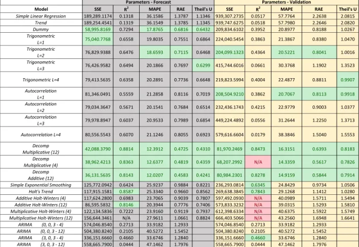
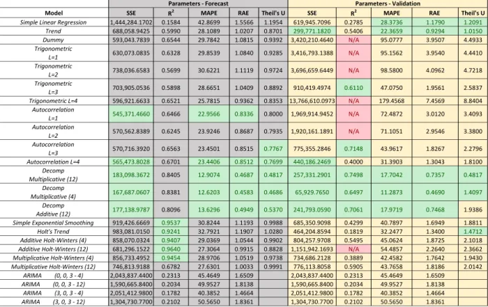
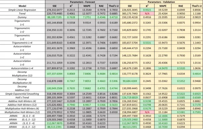
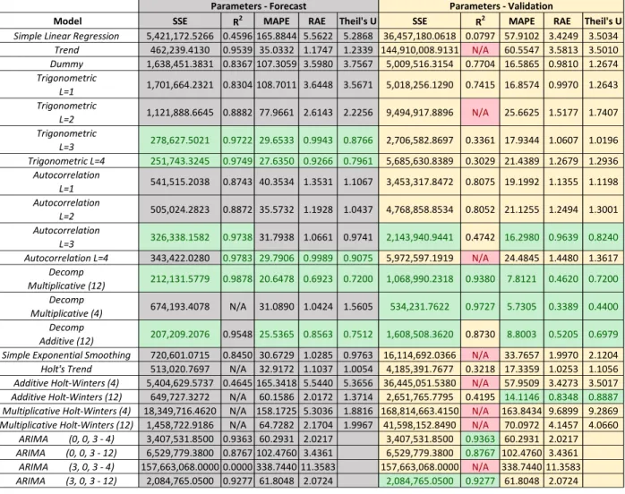
Following the completion of the forecasting models, a chart was built for each variable which listed each forecasting model and the performance of each model based on the five
different parameters (SSE, MAPE, R2, RAE, and Theil’s U). The charts were designed to
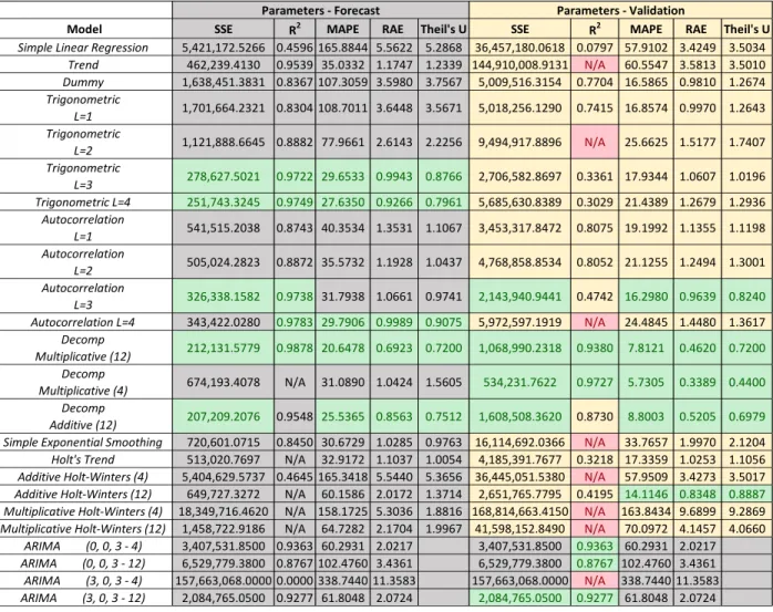
highlight the top five values for each parameter. This allowed the researcher to determine which methods work best for each variable based on the highlighted values. An example of this chart is demonstrated in Table 1 below.
Table 1. Comparison Chart
Model SSE R2 MAPE RAE Theil's U SSE R2 MAPE RAE Theil's U
Simple Linear Regression 5,421,172.5266 0.4596 165.8844 5.5622 5.2868 36,457,180.0618 0.0797 57.9102 3.4249 3.5034 Trend 462,239.4130 0.9539 35.0332 1.1747 1.2339 144,910,008.9131 N/A 60.5547 3.5813 3.5010 Dummy 1,638,451.3831 0.8367 107.3059 3.5980 3.7567 5,009,516.3154 0.7704 16.5865 0.9810 1.2674 Trigonometric L=1 1,701,664.2321 0.8304 108.7011 3.6448 3.5671 5,018,256.1290 0.7415 16.8574 0.9970 1.2643 Trigonometric L=2 1,121,888.6645 0.8882 77.9661 2.6143 2.2256 9,494,917.8896 N/A 25.6625 1.5177 1.7407 Trigonometric L=3 278,627.5021 0.9722 29.6533 0.9943 0.8766 2,706,582.8697 0.3361 17.9344 1.0607 1.0196 Trigonometric L=4 251,743.3245 0.9749 27.6350 0.9266 0.7961 5,685,630.8389 0.3029 21.4389 1.2679 1.2936 Autocorrelation L=1 541,515.2038 0.8743 40.3534 1.3531 1.1067 3,453,317.8472 0.8075 19.1992 1.1355 1.1198 Autocorrelation L=2 505,024.2823 0.8872 35.5732 1.1928 1.0437 4,768,858.8534 0.8052 21.1255 1.2494 1.3001 Autocorrelation L=3 326,338.1582 0.9738 31.7938 1.0661 0.9741 2,143,940.9441 0.4742 16.2980 0.9639 0.8240 Autocorrelation L=4 343,422.0280 0.9783 29.7906 0.9989 0.9075 5,972,597.1919 N/A 24.4845 1.4480 1.3617 Decomp Multiplicative (12) 212,131.5779 0.9878 20.6478 0.6923 0.7200 1,068,990.2318 0.9380 7.8121 0.4620 0.7200 Decomp Multiplicative (4) 674,193.4078 N/A 31.0890 1.0424 1.5605 534,231.7622 0.9727 5.7305 0.3389 0.4400 Decomp Additive (12) 207,209.2076 0.9548 25.5365 0.8563 0.7512 1,608,508.3620 0.8730 8.8003 0.5205 0.6979 Simple Exponential Smoothing 720,601.0715 0.8450 30.6729 1.0285 0.9763 16,114,692.0366 N/A 33.7657 1.9970 2.1204 Holt's Trend 513,020.7697 N/A 32.9172 1.1037 1.0054 4,185,391.7677 0.3218 17.3359 1.0253 1.1056 Additive Holt-Winters (4) 5,404,629.5737 0.4645 165.3418 5.5440 5.3656 36,445,051.5380 N/A 57.9509 3.4273 3.5017 Additive Holt-Winters (12) 649,727.3272 N/A 60.1586 2.0172 1.3714 2,651,765.7795 0.4195 14.1146 0.8348 0.8887
Multiplicative Holt-Winters (4) 18,349,716.4620 N/A 158.1725 5.3036 1.8816 168,814,663.4150 N/A 163.8434 9.6899 9.2869 Multiplicative Holt-Winters (12) 1,458,722.9186 N/A 64.7282 2.1704 1.9967 41,598,152.8490 N/A 70.0972 4.1457 4.0660
ARIMA (0, 0, 3 - 4) 3,407,531.8500 0.9363 60.2931 2.0217 3,407,531.8500 0.9363 60.2931 2.0217 ARIMA (0, 0, 3 - 12) 6,529,779.3800 0.8767 102.4760 3.4361 6,529,779.3800 0.8767 102.4760 3.4361 ARIMA (3, 0, 3 - 4) 157,663,068.0000 0.0000 338.7440 11.3583 157,663,068.0000 N/A 338.7440 11.3583 ARIMA (3, 0, 3 - 12) 2,084,765.0500 0.9277 61.8048 2.0724 2,084,765.0500 0.9277 61.8048 2.0724