Hydrologic Data Assimilation for Operational Streamflow Forecasting

University of Connecticut

OpenCommons@UConn

8-6-2013

Hydrologic Data Assimilation for Operational

Streamflow Forecasting

Feyera Aga Hirpa

[email protected]

Follow this and additional works at:https://opencommons.uconn.edu/dissertations Recommended Citation

Hirpa, Feyera Aga, "Hydrologic Data Assimilation for Operational Streamflow Forecasting" (2013).Doctoral Dissertations. 152.

Hydrologic Data Assimilation for Operational Streamflow Forecasting

Feyera Aga Hirpa

University of Connecticut, 2013

Data assimilation (DA) is a method that optimally combines imperfect models and uncertain observations to correct model states using new information acquired from the incoming observations. In recent years, DA has been extensively used for improving the uncertainty of hydrologic prediction, largely due to the emergence of advanced remote sensing tools for observations of soil moisture, river discharge and precipitation. Several DA methods have been explored in hydrology; however the choice and the effectiveness of a specific DA method may vary depending on the model and the observation.

The goal of this dissertation study was reducing streamflow forecast uncertainty, and was carried out in three parts. First, the effectiveness of four different DA methods (ensemble Kalman filter (EnKF), particle filter (PF), Maximum Likelihood Ensemble Filter (MLEF) and

variational method (VAR)) for improving streamflow forecasting were evaluated. In-situ

discharge was assimilated into The United States National Weather Service (NWS) river forecasting model (Sacramento Soil Moisture Accounting model (SAC-SMA)) for Greens

Bayou basin (with area of 178km2), in eastern Texas. The results indicate that all the four DA

methods enhanced the short lead time forecast when compared to the model without the data assimilation; however the performances of each method vary with flow magnitude and longer lead time forecasts. Overall, the PF and MLEF performed superior to other DA algorithms across all flow regimes.

In the second part of this thesis, the value of satellite-based soil moisture retrievals for enhancing river discharge was assessed. Surface and root zone satellite-based soil moisture retrievals from AMSR-E (passive microwave) and ASCAT (active microwave) sensors were separately assimilated into the SAC-SMA model in Greens bayou using ensemble Kalman filter. Two different data assimilation experiments were carried out over a period of four years (2007 to 2010): updating the soil moisture state of the SAC-SMA model and combined correcting of soil moisture and total channel inflow (TCI) of the model. It was found that the remotely-sensed soil moisture assimilation reduced the discharge RMSE compared to the open loop for both assimilation schemes, and there was no appreciable difference between surface and root zone soil moisture results, as well as between the AMSR-E and ASCAT results. Furthermore, the dual correcting of soil moisture and TCI produced lower river discharge RMSE.

In the third part, the utility of passive microwave-based river width estimates for river discharge nowcasting and forecasting were assessed for two major rivers, the Ganges and Brahmaputra, in south Asia. Multiple upstream satellite observations of river and flood plains were used to track downstream flood wave propagation, and using a cross-validation regression model, the downstream river discharge was forecasted for lead times up to 15 days. The results showed that satellite derived flow signals were able to detect the propagation of a river flow wave along both river channels. And the approach also provided better discharge forecasts at downstream location compared to a purely persistence forecast, especially for high flows when the water spills out of the river bank. Overall, it was concluded that satellite-based flow estimates are a useful source of dynamical surface water information in regions where there is a lack of ground discharge data.

Hydrologic Data Assimilation for Operational Streamflow Forecasting

Feyera Aga Hirpa

B.Sc., Jimma University, 2004

M.S., University of Connecticut, 2009

A Dissertation

Submitted in Partial Fulfillment of the

Requirements for the Degree of Doctor of Philosophy

at the

University of Connecticut

2013

Copyright by Feyera Aga Hirpa

2013

APPROVAL PAGE Doctor of Philosophy Dissertation

Hydrologic Data Assimilation for Operational Streamflow Forecasting

Feyera Aga Hirpa, B.Sc., M.S.

Major Advisor__________________________________________________ Mekonnen Gebremichael Associate Advisor_______________________________________________ Thomas M. Hopson Associate Advisor_______________________________________________ Emmanouil N. Anagnostou Associate Advisor_______________________________________________ Amvrossios C. Bagtzoglou Associate Advisor_______________________________________________ Guiling Wang

University of Connecticut

2013

To

Aabbo

(Dad) and

Ayyaa

(Mom)

ACKNOWLEDGEMENT

First of all, I would like to give glory to the LORD, the Almighty God, for His guidance, protection, and purpose in my life.

Next I would like to thank my major advisor, Dr. Mekonnen (Moke) Gebremichael, for believing in me from the very beginning and providing me with the opportunity to pursue my graduate studies at UConn. I appreciate the full freedom I enjoyed to choose the research topic of my interest, as well as the remarkable patience and unconditional support you showed to me. Thank you, Moke!

I am deeply grateful to Dr. Thomas M. Hopson, who has been greatly supportive of me at all times including during my visits to National Center for Atmospheric Research (NCAR). Tom showed me tremendous kindness and unreserved professional support. I specially acknowledge his ideas for the work on operational river flow forecasting in Bangladesh (chapter 4 of this dissertation). I am also very thankful to Dr. Emmanouil N. Anagnostou for introducing Kalman filtering to me and encouraging me to learn more about data assimilation. My sincere gratitude also goes to Dr. Amvrossios C. Bagtzoglou and Dr. Guiling Wang for serving in my PhD committee. Thank you all.

My deepest gratitude goes to my parents for their unconditional love and support. I am forever thankful to my father, Aga Hirpa Kitil, and my mother, Kibitu Sori, who both have been a source of motivation and an example of hard work. My sisters and brother also have been great support all the times. Thank you all very much.

I am grateful to fellow graduate students at UConn with whom we had lots of memories. These include Menberu (and his family), Dawit, Viviana, Carlo, Dan, Uday, and all others.

TABLE OF CONTENTS

II. Chapter 2: Hydrologic Data Assimilation for Streamflow Forecasting: Implementation and Comparative Evaluation of EnKF, PF, MLEF and VAR Methods………..……..……...….…10

2.1. Introduction………..……….………10

2.2. Study Area, Hydrologic Model and Data………..…….…….…..……14

2.3. Flow Variation with Model State……….…….………17

2.4. DA Methods and Implementation……….…….………...20

2.4.1. Ensemble Kalman filter……….………...…21

2.4.2. Particle filter……….………23

2.4.3. Variational method……….……….…….25

2.4.4. Maximum likelihood ensemble filter…….………...………...…26

2.5. Description of the DA experiments……….……….…………...27

2.5.1. Experiment setup……….……….27

2.5.2. Model and measurement errors………29

2.6. Evaluation methods……….………..30

2.7. Results and Discussions……….………….…..31

2.8. Conclusions……….………..…39

III. Chapter 3: Assimilation of Satellite Soil Moisture Retrievals into Hydrologic Model for Improving River Discharge ……….……41

3.1.Introduction ……...………..………...41

3.2.Study Area, Model and Data………...………44

3.2.1. Study Area………..………...……44

3.2.2. Hydrologic model and inputs……….……..….………46

3.2.3. AMSR-E Soil Moisture data……….……….…...…48

3.2.4. ASCAT Soil Moisture data……….………….….…49

3.3.Method………..………….…….50 3.3.1. CDF mapping……….………...50 3.3.2. DA experiment……….……….51 3.4.Results………..……….. 54 3.4.1. AMSR-E assimilation……….………..54 3.4.2. ASCAT assimilation……….………56

3.4.3. Comparison of the STU………….………58

3.5.Conclusions……….………59

IV. Chapter 4: Satellite River Width Estimates for River Discharge Forecasting: Application to Major Rivers in South Asia…….………61

4.1.Introduction..……….………61

4.2.Study region and datasets……….……….65

4.2.1. Study region……….………...……….……65

4.2.2. Datasets……….………...…67

4.3.Satellite-derived flow signals……….……...69

4.3.1. Correlation with gauge observations……….…..…69

4.3.2. Variation of flow time with flow path length………..…69

4.3.3. Limitations of the flow propagation model…...……….….…74

4.4.Selection of satellite flow signals for discharge estimation………...76

4.5.Results of discharge nowcasts and forecasts……….…79

4.5.1. Discharge nowcasts and forecasts using satellite river flow signals only………..…79

4.5.2. Discharge forecasts using combined SDF signals and persistence..83

4.6.Water level from discharge forecast……….88

4.7.Conclusions………..…….92

V. Chapter 5: Summary and Future Research………94

5.1.Summary………..94 5.2.Future research………96 APPENDIX A: ………...………...99 APPENDIX B: ………...………..100 APPENDIX C: ...………...…………...101 BIBLIOGRAPHY: ………...104

LIST OF FIGURES

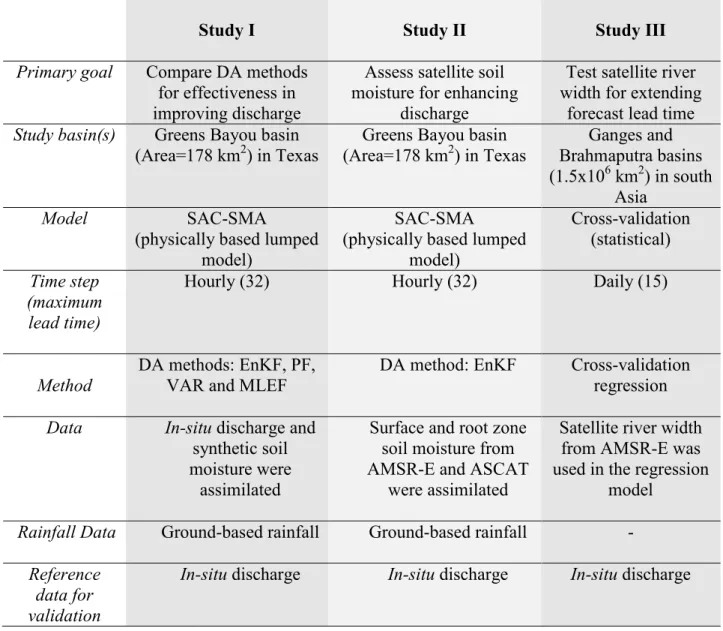
Figure 2.1. Greens Bayou basin in eastern Texas. The basin has a catchment area of 178 km2...15 Figure 2.2. Schematic diagram of the SAC-SMA model. The model has two soil zones: upper

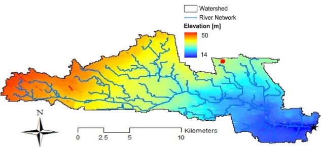
and lower zone. There are four flow components: Surface Saturation-excess Runoff (SSR), Surface Infiltration-excess Runoff (SIR), Sub-surface Interflow (SSIF) and Base Flow (BF). The aggregation of the flows produces Total Channel Inflow (TCI), which generates discharge after channel routing……….17 Figure 2.3. The log-log plot of the relationship between the four flow components and the soil

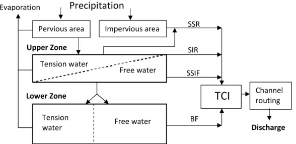
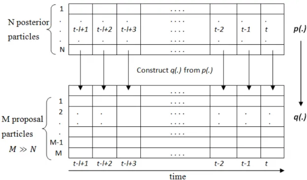
moisture states of the SAC-SMA. The surface infiltration-excess runoff (SIF) component is the most dominant during the high flow for the study basin, followed by the surface saturation-excess runoff (SSR) component. Note that the SIR and SSR are not correlated with the soil moisture states. On the other hand, the sub-surface interflow (SSIF) and the base flow (BF) increase in proportion to the upper zone and lower zone free water contents respectively………..19 Figure 2.4. Chart showing construction of the proposal distribution in the particle filtering

algorithm. The proposal distribution q(.) at time t-l+i is randomly sampled from the

posterior density p(.) at the corresponding time as shown by the arrows. The indices t

and l are, respectively, the time of assimilation and width of the empirical unit

hydrograph. The index I varies from one to l………...25

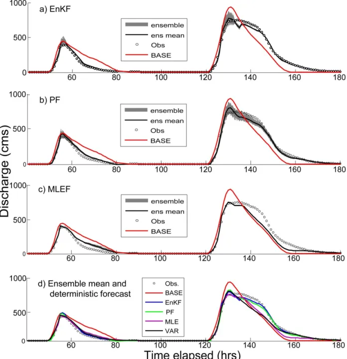
Figure 2.5. Time series display of 1-hour lead forecast using SAC-SAM model without DA (BASE) and model aided with DA. The top three panels are for ensemble forecasts: a)

EnKF, b) PF and c) MLEF. The lower panel compares the deterministic forecasts (BASE and VAR) with the mean of the ensemble forecasts. The largest peak shown is the extreme flooding caused by Tropical Storm Allison in year 2001………....34 Figure 2.6. The comparison of Continuous Ranked Probably Skill Score (CRPSS) for different flow ranges: a) overall flow from January 1996 to March 2005, and for flows exceeding

b) the 75th quantile (1.90 m3/s), c) 95th quantile (12.40 m3/s), and d) 99th quantile (51.54

m3/s). For deterministic forecast, VAR, the CRPSS can be viewed as the mean absolute

error skill score……….……….37 Figure 2.7. Normalized Root Mean Square Error (normalized by mean) of the forecast shown

for different flow regimes: a) low flow (<Q25, 25th climatological quantile), b)

moderate flow (between Q25 and Q75), c) high flow (between Q75 and Q95), d) extreme flow (exceeding Q95)………38

Figure 3.1. Greens Bayou basin (Area=178 km2) located in eastern Texas. a) center of satellite

soil moisture grids for AMSR-E (three green dots) and ASCAT (five purple dots. b) Land use/cover of the basin extracted from National Land Cover Data (NLCD) 2006……….…45 Figure 3.2. Schematic diagram of the SAC-SMA model with two soil zones (upper and lower

zone) and four flow components. The flow components (SSR, SIR, SSIF and BF) are aggregated to produce the Total Channel Inflow (TCI). River discharge is generated after channel routing of TCI using unit hydrograph……… 47 Figure 3.3. The AMSR-E, ASCAT and SAC-SMA simulated soil moisture for a) upper and b)

lower soil zones as defined by the SAC-SMA model. The satellite soil moisture retrievals are mapped to SAC-SMA model space using CDF matching approach. The

surface soil moisture (SSM) for the upper zone and the root zone (RZ) soil moisture for the lower zone are shown……….…52 Figure 3.4. River discharge improvement from assimilation of AMSR-E soil moisture….….56 Figure 3.5. Similar to Figure 4, except a) ASCAT surface soil moisture (ASCAT-SSM) and b)

ASCAT root zone (ASCAT-RZ)………..57 Figure 3.6. Comparison of the discharge RMSE after the soil moisture state and TCI…..…59 Figure 4.1. The Brahmaputra and Ganges Rivers in South Asia. The satellite flood signal

observations are located on the main streams of the Brahmaputra (top right) and the Ganges (bottom left) rivers. The observation sites are shown in small dark triangles and they are labeled by the GFDS site ID (see Table 4.1)………..…66 Figure 4.2 a) Correlation versus lag time between daily in-situ streamflow and upstream

satellite flood signals, SDFs (only 3 shown here) and gauge discharge at Hardinge Bridge along the Ganges River in Bangladesh. As expected, the lag time at which peak correlation occurs (shown as a dark dot) is greater for longer flow path lengths (FPL)

from the gauge at Hardinge. b). Correlation versus lag time between daily in-situ

streamflow and upstream satellite flood signals, SDFs (only 3 shown here) and gauge discharge at Bahadurabad along the Brahmaputra River………..71 Figure 4.3 a). Plot of flow time (as estimated from the satellite flood signal data) versus

distance from the satellite flow detection point to the outlet (Hardinge bridge station) of the Ganges River. The flow time is the lag time at which the peak correlation occurred, as shown in Figure 2a. The flow speed estimated from the slope of the fitted line is 2.85 m/s. b). Same as Figure 4.3a., but for Brahmaputra river. The flow speed estimated from the slope of the fitted line is 9.85 m/s……….………73

Figure 4.4 a) Lagged correlation map of daily satellite-derived flow signals calculated against the discharge observation at Hardinge Bridge for Ganges River. The horizontal axis shows the satellite flood signal sites (see Figure 1) arranged in the order of increasing flow path length and the vertical axis shows lag time (days). b) Same as Figure 4a, but for Brahmaputra………..…………..78 Figure 4.5. Daily time series of observed river discharge, nowcast and forecast (for selected

lead time) based on the river flow signal observed from satellite. The upper panels show 2003 (5a) and 2007 (5b) results for Ganges River at Hardinge bridge station in Bangladesh. The lower panels are 2004 (5c) and 2007 (5d) plots for Brahmaputra at Bahadurabad. Five and ten day lead time forecast are selectively shown in these plots. The details of the satellite-derived flow signals used for the nowcasting has been presented in Table 4.1………..….80 Figure 4.6. The Nash-Sutcliffe coefficient versus forecast lead time for Ganges and

Brahmaputra Rivers. Only satellite-derived flow signals were used for the forecast. The Nash-Sutcliffe coefficients were calculated for the whole time period of record (December 8, 1997 to December 31, 2010)……….…83 Figure 4.7. Daily time series based on satellite derived signals and persistence (SDF+PERS)

based river discharge forecast at selected lead times shown against observation during the 2003 (6a) and 2007 (6b) flooding of Ganges River at Hardinge bridge station in Bangladesh. The 2004 (6c) and 2007 (6d) forecasts for Brahmaputra at Bahadurabad are also shown………..….84 Figure 4.8. a) The RMSE of persistence (PERS), Autoregressive moving-average (ARMA),

Brahmaputra rivers. The SDF+PERS forecast is better than the PERS for both rivers and the ARMA expectedly beats the PERS. The SDF+PERS forecast has lower RMSE than ARMA for Brahmaputra, but this is not the case for Ganges. The SDF-only nowcasts (dark points on the vertical axis) indicates that the satellite discharge estimate (see Figure 5) is at least as good as 7 day lead time forecast that is aided by in situ discharge. b) The root mean square error (RMSE) skill score of SDF+PERS forecast versus forecast lead time for the Ganges and the Brahmaputra Rivers discharge forecasts. The skill scores were calculated for the whole time period of record (December 8, 1997 to December 31, 2010)……….86 Figure 4.9. Root mean square error (RMSE) of monsoon water level forecast for the Ganges

and the Brahmaputra Rivers shown for different forecast lead times. The error increases with lead time for both rivers, and it is larger for the Ganges compared to the Brahmaputra……….………..88 Figure 4.10 a) RMSE of water lever forecast for Ganges River shown for different flow

regimes during monsoon season (June-October). The water level is obtained from discharge forecast using the rating curve equations. The water level forecast errors decrease with increasing flow magnitude indicating that the PMW sensors detect floods more accurately when the river overflows the bank, inundating wider area, as opposed to low flow where the flow remains in the river bank. B). Same as Figure 4.10a except for Brahmaputra River……….…90 Figure B1. SAC-SMA’s empirical unit hydrograph for Greens Bayou basin…….…………100 Figure C1. Map showing the sites selected by the cross-validation regression model [section 4.4

described in Table 1, with increasing FPL from left to right. Meanwhile, the numbers on the vertical axis denote the lead time forecast and the nowcast is represented by lead time of ‘0’. The color map shows the number of times (including the lagged observations) data from a SDF site is used in the regression model……….102 Figure C2. Same as Figure C1 except for Brahmaputra River………..……….103

LIST OF TABLES

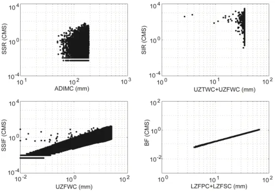
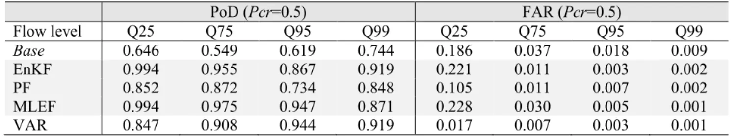
Table 1.1. Summary of the three parts of the dissertation research……….……..5 Table 2.1. Summary of probability of detection (PoD) and False alarm rate (FAR) of the DA

methods for different climatological flow quantiles at 1-hour lead time forecast. The

quantiles for the study basin have the following flow magnitude: Q25= 0.934 m3/s;

Q75= 1.90 m3/s; Q95= 12.40 m3/s; and Q99 = 51.54 m3/s. PoD for ensemble forecasts

in the case of Pcr=0.5 describes the probability that more than half of the ensembles

detected an event given that it occurred. And FAR is the probability that more than half

of the ensembles (Pcr=0.5) falsely reported occurrence of an event. ………..36

Table 2.2. Same as Table 2.1, but for forecast lead time of 6-hours. ………36 Table 2.3. Same as Table 2.1, but for forecast lead time of 24-hours………36 Table 4.1. Details of the satellite-derived flow signals (“MagnitudeAvg” in the GDACS

database) used for the study. The site ID, latitude, longitude and flow path length (FPL) are provided. The period of record for all the data, including the satellite flood signals and the gauge discharge observations at Hardinge Bridge and Bahadurabad is December 8, 1997 to December 31, 2010. ……….68 Table A1. The sixteen SAC-SMA parameters and their calibrated values for the Greens Bayou

Chapter 1

Introduction

1.1. Background

In order to adequately address uncertainty in hydrologic modeling, it is fundamental to understand, quantify and reduce hydrologic uncertainty (Liu and Gupta, 2007). Understanding uncertainty in hydrologic prediction involves identifying the sources of uncertainty, which includes errors in model structure, parameters, initial conditions, inputs and observations often used for model calibration. The model structure determines how the model inputs (e.g. rainfall) interact with model state (e.g, soil moisture), and defines how the model outputs (e.g., discharge) respond to changes in the model states. Consequently, error in the model structure has a direct impact on the uncertainty level of the model output. The model parameters represent the time-invariant characteristics of a watershed such as soil porosity, hydraulic conductivity, and other physical properties that do no change over long period of time. They are empirical representations of the watershed characteristics, and errors in the parameter estimation result in large errors in the model output (Liu et al., 2005).

Model initial condition (e.g., antecedent soil moisture) is another factor that has direct implication for hydrologic uncertainty. Antecedent water content of the soil impacts the partitioning of rainfall into runoff and infiltration, as well as it influences the partitioning of the incoming solar energy into latent and sensible heat components. Consequently, the magnitude of the overland flow is directly, but nonlinearly, affected by the initial soil moisture estimate. Thus, representing the soil moisture state with better accuracy is an important step towards reducing hydrologic prediction uncertainty. Additionally, errors in rainfall (input) and streamflow data used for model calibration and verification need to be minimized in order to reach a goal of

reducing hydrologic prediction uncertainty. The subject of this dissertation study is not quantifying each of the errors in the model structure, parameters or data, but it is focused instead on reducing the hydrologic uncertainty by optimally combining ground-based data, satellite

observations and hydrologic models.

In the past few years, data assimilation (DA) has gained much popularity as a tool for reducing hydrologic uncertainty. DA is a method which optimally combines imperfect models with uncertain data to “correct” model states and, as a result, reduce uncertainty of the model prediction. It takes into account the relative errors of the model and the data for the process of optimally merging the two. Several studies have used various data assimilation approaches in hydrologic applications by optimally combining model and observations in order to improve the skills of the streamflow forecasting. A detail literature review on this is provided under section 2.1 of this dissertation. The most commonly used methods in hydrology are variational methods (VAR), ensemble Kalman filters (EnKF) and particle filters (PF). Maximum likelihood ensemble filters (MLEF) has been used in meteorology but it is fairly new DA method in hydrologic applications. All DA methods have their own advantages and disadvantages, but their differences mainly arise from the error introduced in the approximation of the non-linear model, computational cost and their assumptions of the model and observation errors to provide an optimal solution. The design of a specific DA method also depends on the model structure, and hence the implementation of a DA method should be adaptable to the model under consideration.

As far as assimilation of soil moisture data is concerned, though there has been significant advancement in acquiring soil moisture at higher spatial and temporal scales from space, at the present stage the global soil moisture data is far from complete. Ground-based soil moisture observations are sparse and not usually representative of the large spatial scale of river

catchment. As a matter of fact, the total number of ground stations currently reporting to the

global in-situ soil moisture database, operated by the International Soil moisture Network at the

Vienna University of Technology, is less than 1,500, with 57% of those stations coming from one nation, the United States (see http://ismn.geo.tuwien.ac.at/networks/). Global land surface models could produce soil moisture over larger spatial scales, but separate models often produce different soil moisture values even when identical forcings were used to run the models (Entin et al., 1999), and they usually fail to reproduce the true soil moisture.

Satellite-based soil moisture retrievals have been recently shown to be useful for several hydrometeorological applications, as reviewed in chapter 3 of this dissertation. Particularly, advanced soil moisture retrievals from passive and active microwave satellite remote sensing are now globally available at fine spatial and temporal scales needed for hydrologic applications. The most commonly used sensors for soil moisture are the Advanced Microwave Scanning Radiometer for Earth observing system (AMSR-E) onboard the Aqua satellite and the Advanced SCATterometer (ASCAT) onboard the MetOp (Meteorological Operational) satellite. Soil

moisture estimates derived from these sensors have been evaluated through comparison with

in-situ or model simulated soil moistures (see chapter 3 for details) and reported to correspond

significantly well with the reference soil moisture. Higher quality soil moisture retrievals with higher spatial and temporal resolution are expected when NASA’s Soil Moisture Active Passive (SMAP) mission dedicated exclusively to soil moisture is launched in 2014 (Entekhabi et al., 2010).

A few studies recently have assimilated remotely-sensed soil moisture into rainfall-runoff models for a purpose of improving discharge prediction (a subject of chapter 3) using sequential data assimilation. But since the relationship between soil moisture and discharge is highly

nonlinear, accurate estimation of soil moisture alone doesn’t solve the discharge uncertainty problem (Hirpa et al., 2013). To address this, dual soil moisture state and antecedent precipitation index (API) updating was introduced by Crow et al. (2005). The dual state and API updating using soil moisture was shown to be more effective in improving river discharge when tested using synthetic soil moisture (Crow and Ryu, 2009), but it was yet to be tested using real data from satellite retrievals.

Another remotely-sensed data that can be used to reduce river discharge prediction error is upstream river width retrieved from satellite passive microwave sensors (see chapter 4 for details). The European Joint Research Center (JRC-Ispra, http://www.gdacs.org/floodmerge/), in collaboration with the Dartmouth Flood Observatory (DFO) centered at Dartmouth College (http://www.dartmouth.edu/~floods/), produces daily near real-time river flow signals from satellite brightness temperature, along with flood maps and animations, at more than 10,000 monitoring locations for global major rivers. The river flow data is largely useful in large transboundary rivers or the developing nations where there is a limited sharing or availability of ground-based river discharge measurements. The attractive aspect about the microwave signal is that at 36.5GHz it does not suffer much from cloud interference, and has been demonstrated to be useful to estimate river discharge changes, river ice status, and watershed runoff worldwide (Brakenridge et al., 2007).

The purpose of this study was to reduce the hydrologic uncertainty by optimally merging the in-situ, remotely-sensed observations and hydrologic models using data assimilation. This

was carried out in three separate parts as summarized in Table 1.1. First (“Study I”), the in-situ

discharge was assimilated into National Weather Service’s (NWS) Sacramento Soil moisture

in Texas. Four different DA methods, EnKF, PF, VAR and MLEF, were tested for effectiveness in improving river discharge.

Reducing uncertainty in river discharge

Study I Study II Study III

Primary goal Compare DA methods

for effectiveness in improving discharge

Assess satellite soil moisture for enhancing

discharge

Test satellite river width for extending

forecast lead time

Study basin(s) Greens Bayou basin

(Area=178 km2) in Texas

Greens Bayou basin

(Area=178 km2) in Texas Ganges and Brahmaputra basins (1.5x106 km2) in south Asia Model SAC-SMA

(physically based lumped model)

SAC-SMA

(physically based lumped model) Cross-validation (statistical) Time step (maximum lead time)

Hourly (32) Hourly (32) Daily (15)

Method

DA methods: EnKF, PF, VAR and MLEF

DA method: EnKF Cross-validation

regression

Data In-situ discharge and

synthetic soil moisture were

assimilated

Surface and root zone soil moisture from AMSR-E and ASCAT

were assimilated

Satellite river width from AMSR-E was used in the regression

model

Rainfall Data Ground-based rainfall Ground-based rainfall - Reference

data for validation

In-situ discharge In-situ discharge In-situ discharge

Second (“Study II”), surface and root zone satellite soil moisture retrievals from AMSR-E and ASCAT sensors were assimilated into SC-SMA model using the AMSR-EnKF approach. Two different DA approaches were compared based their degree of discharge improvement. Third (“Study III”), the utility of using passive microwave derived river width estimates for near-real time river flow estimation and forecasting for the Ganges and Brahmaputra rivers were examined. The river width was estimated from the brightness temperature measured by sensors on the AMSR-E, but since AMSR-E is no longer functional due to antenna problem as of October 2011, the brightness temperature is being acquired from the Tropical Rainfall Measuring Mission (TRMM) satellite.

1.2

. Objectives

This research aims to meet the following scientific objectives:

i. Test which data assimilation technique provides more reliable result for operational

streamflow forecasting. All the DA methods have their own strengths and limitations

depending on the characteristics of the data assimilation problem. For example, factors such as flexibility in the error model assumptions, nonlinearity of the model, computational cost, number of ensembles needed to achieve satisfactory result, and the difficulty of practical implementation for large scale problems need to be taken into consideration to obtain (sub)optimal results when using a specific DA method for hydrologic applications. In this research we will implement and compare the Ensemble Kalman Filter (EnKF), Particle Filter (PF), Variational method (VAR) and Maximum

Likelihood Ensemble Filter (MLEF) for the assimilation of in-situ discharge observation

ii. Evaluate the contribution of satellite-based soil moisture retrievals for enhancing river discharge of the SAC-SMA model.Surface and root zone soil moisture retrievals

from AMSR-E and ASCAT sensors were separately assimilated into SAC-SMA model. Two different DA approaches were undertaken: soil moisture state updating, and dual soil moisture and TCI updating. The resulting discharge improvement was evaluated through comparison with open loop and ground discahrge.

iii. Assess the utility of near-real-time satellite-based estimates of upstream river width for improving accuracy and extending the lead time of streamflow forecast.

Near-real-time river width estimates were used for tracking flood waves and improving the streamflow forecast along the Ganges and Brahmaputra rivers in South Asia. The river width data were derived from the passive microwave sensor (AMSR-E) and TRMM sensors. These estimates are provided globally by the Dartmouth Flood Observatory (Brakenridge et al., 2007) and the Joint Research Centre (JRC) of the European Commission (De Groeve et al., 2006).

1.3. Research Questions

Each of the three studies raised and attempted to find answers to the following scientific questions. In some cases, when the findings were not adequate to provide full answer, the study pointed to the gap for possible research directions. The summary of the studies are presented in Table 1.1.

Study I: evaluation of different DA methods

• _{Which of the DA algorithms (EnKF, PF, VAR or MLEF) enhances the river discharge}

• _{Which approach, ensemble-based or deterministic, performs better for various lead times}

and flow magnitudes?

• _{What is the relationship between soil moisture and river flow and how does updating soil}

moisture state improve the streamflow forecasting? Study II: assimilation of satellite-based soil moisture

• How do active and passive microwave satellite soil moisture retrievals improve the river

discharge when assimilated into rainfall-runoff model?

• How does the degree of discharge improvement differ between the surface and root zone

satellite soil moisture?

• Do the dual soil moisture state and the TCI correcting of the SAC-SMA model perform

better than soil moisture only updating? Study III: use of satellite-based river width estimates

• _{Can satellite-based river width estimates from passive microwave be used to track flood}

wave propagation along river channels?

• How much gain in forecast lead time can be achieved by using upstream river inundation

from satellite?

• What is the skill of the river discharge forecast based on upstream river width from

satellite compared to persistence and ARMA model forecasts?

The reminder of the thesis is organized as follows. Chapters 2 presents the “Study I” including the literature review on DA in hydrology, study area, methods, results and discussions. Likewise, Chapter 3 and 4 present, respectively, the full descriptions of the “Study II” and “Study III”. Results of the study are summarized in Chapter 5.

As summarized in Table 1.1, the focus of the “Study I” was comparing several DA algorithms for improving streamflow forecast. “Study II” was on assessing satellite-based soil moisture retrievals for enhancing river discharge, and “Study III” tests the utility of satellite river width for tracking flood wave propagation and improving river discharge forecasting skill.

Chapter 2

Hydrologic Data Assimilation for Streamflow Forecasting: Implementation and

Comparative Evaluation of EnKF, PF, MLEF and VAR Methods

2.1.

Introduction

Accurate and reliable hydrologic forecast is critical for operational streamflow forecasting in flood disaster mitigation, dam operation and other water resources management applications. Hydrologic prediction uncertainties originate from one or combinations of the following error sources: hydrologic model structure and parameters, model forcing (amount/rate and spatio-temporal distribution), model initialization (e.g., soil moisture states), and historical discharge observations often used for model calibration. Several studies have analyzed these sources of uncertainties and methods of dealing with them (e.g., Restrepo, 1985; Kuczera and Parent, 1998; Kavetski et al., 2006; Vrugt et al., 2003; Wagner et al., 2003; Montanari and Brath, 2004; Ajami et al., 2007; Liu and Gupta, 2007; Moradkhani and Sorooshian, 2008; Salamon and Fayen, 2009; Renard et al., 2010; Franz and Hogue, 2011; Mendoza et al., 2012).

Hydrologic uncertainty problems can be mitigated through data assimilation (DA), which is a technique that optimally combines the hydrologic model outputs with independent observations, and modifies certain states of the model by taking into account the relative errors of the model outputs and the observations. In the past few years, DA has emerged as a powerful tool in hydrologic forecasting due to a number of factors, such as, increasing availability of observations (e.g., from satellite remote sensing), improved DA methods, and need for higher hydrologic forecasting accuracy. Liu et al. (2012) reviewed DA studies over

into land surface models. Of our particular interest for hydrologic applications are

assimilation of in-situ discharge (e.g., Seo et al., 2003, 2009; Moradkhani et al., 2005; Weerts

and El Serafi, 2006; Clark at al., 2008; Lee et al., 2011; 2012), in-situ soil moisture (e.g.,

Aubert et al., 2003; Lee at al., 2011), satellite soil moisture (e.g., Pauwels et al., 2001; Reichle et al., 2002, 2008; Parajka et al., 2006; Crow and Ryu, 2009; Draper et al., 2011; Hain et al., 2011; Brocca et al., 2010, 2012, Maggioni et al., 2013), and satellite-based water elevation (e.g., Montanari et al., 2009, Biancamaria et al., 2011).

A number of DA methods have been applied in operational riverflow forecasting mainly focusing on state updating, parameter estimation, and/or model error updating (as reviewed by Liu at al., 2012). The most commonly implemented DA methods in hydrology are: Kalman filter (with its various modifications), variational DA methods and particle filter. The standard Kalman filter (Kalman, 1960) is a linear recursive optimal filter that combines imperfect model and uncertain observation to estimate the state evolution of a dynamic system and propagation of covariance error matrix from one time step to the next. The Extended Kalman filter (EKF) is a modified version of the standard Kalman filter to accommodate the nonlinearity of state space and measurement models. The EKF has been used for state estimation in hydrology (e.g., Katinadis and Bras, 1980; Reichle et al., 2002), but it was also noted that the linear approximation of a nonlinear model could make the filter unstable and computationally expensive to implement. A more commonly utilized state updating method in hydrology is Ensemble Kalman filter (EnKF) which was first introduced by Evensen (1994). The EnKF is Monte Carlo based filter in which the state is represented by ensemble realizations of the true state, where the ensemble mean is considered as the state estimate and the model error is approximated by the ensemble variance. At the initialization

step, the ensembles are sampled from a priori distribution, and then during a prediction phase

each member evolves independently following the state space model. Then, whenever new observations are available, the posterior state (more certain estimate of the true state) is estimated by updating each ensemble member individually based on the combination of information obtained from the observation and the model itself. These sequences are iteratively repeated forward until present time (for Kalman smoothing) or to the future (for Kalman filtering). The EnKF has been used in hydrologic applications in previous studies (e.g., Reichle et al., 2002; 2008; Vrugt et al., 2006; Pan et al., 2007; Clark et al., 2008, and Draper et al., 2012, to name a few).

Another Monte Carlo based DA method recently gaining more attention in hydrology is the particle filter (PF) (Doucet et al., 2000; Arulampalam et. al., 2002; Moradkhani et al., 2005; Weerts and El Serafi, 2006; Pan et al., 2007; Noh et al., 2011; DeChant and Moradkhani, 2012; Plaza et al., 2012). In PF, ensemble members (particles) are initialized

from a priori distribution and each particle is assigned with weights representing the

corresponding probability of a particle. During the prediction step, in a similar fashion to the EnKF, each particle separately evolves following the model dynamics. Then, when new observations are available, a new set of weights are calculated for each member based on the likelihood of the observation, where the weights represent the posterior probability distribution of the state. The main differences between the EnKF and PF are: there is no direct state updating in PF, and the PF does not make Gaussian assumption for the model and observation errors, which theoretically makes it more appropriate for hydrologic applications where the error characteristics are typically far from Gaussian.

Variational data assimilation (VAR) is a batch-processing method widely used in meteorology and hydrology (Bouttier and Courtier, 1999; McLaughlin, 2002; Reichle et al., 2002; Seo, et al., 2003, 2009; Lee et al., 2011, 2012). It solves a minimization problem over a certain time window (commonly referred to as assimilation window) in which constrained nonlinear minimization algorithms are applied to a cost function consisting of model and observation errors. The cost function is setup in such a way that the model and observations with larger error values (deviation from the truth) are penalized, and the constraints are enforced for a purpose of keeping the entities within physically meaningful bounds. Zupanski (2005) transformed the cost minimization technique from model space to ensemble space by combining the maximum likelihood estimation from Kalman filtering with the state estimation using the cost function minimization methods. The method was introduced as the maximum likelihood ensemblefilter (MLEF), but has not yet been tested for hydrologic applications.

All the DA methods have their own strengths and limitations depending on the characteristics of the data assimilation problem. For example, factors such as flexibility in the error model assumptions, nonlinearity of the model, computational cost, number of ensembles needed to achieve satisfactory result, and the difficulty of practical implementation for large scale problems need to be taken into consideration to obtain (sub)optimal result when using a specific DA method for hydrologic applications.

The purpose of the present study was to implement and comparatively evaluate the effectiveness of four DA methods for improving real-time operational hydrologic forecasting. Specifically, we aim to address the following research questions: which algorithm, sequential or batch-processing, enhances the forecast better? Which approach, ensemble-based or

deterministic, performs better for various lead times? How does updating soil moisture state improve the streamflow forecasting? To address these questions, we first analyzed the streamflow variation with soil moisture states of the SAC-SMA model for the study basin. Then, we utilized different algorithms/approaches (sequential, batch-processing,

ensemble-based and deterministic) for data assimilation of in-situ discharge into the Sacramento Soil

Moisture Accounting Model (SAC-SMA) (Burnash et al., 1973) for streamflow forecasting of a small watershed in the Unites States.

Our study extends the previous DA comparison studies (e.g., Weerts, 2006; DeChant and Moradkhani, 2012) by including more methods (VAR and MLEF), and introduces a new method for creating importance density for Sampling Importance Resampling (SIR) algorithm of the sequential Monte Carlo in the PF. The DA methods were independently used to update the dynamic model states at each assimilation time, while the model parameters were assumed to be time-invariant and estimated off-line of the DA. We adopted the SAC-SMA model parameters estimated for the study basin by Seo et al. (2009) using the Adjoint-Based Optimizer (AB_OPT) algorithm.

The remainder of this chapter is organized as follows. Section 2.2 presents an overview of the study area, hydrologic model and data. Section 2.3 analyzes the variation of flow components as a function of soil moisture states of the model. Section 2.4 describes the DA methods and implementations. In section 2.5, the experiment setup is presented. Evaluation methods and results are discussed in sections 2.6 and 2.7 respectively. Finally, conclusions were summarized in section 2.8.

The study area is the Greens Bayou watershed located in Harris County, Texas (See Figure 2.1). It is one of the several basins in NWS West Gulf River Forecast Center (WGRFC) chosen for experimental implementation of variational data assimilation (Seo et al.,

2003; 2009). The basin has a drainage area of 178 km2 with the outlet (USGS site ID of

‘08076000’) located at about 17 km northeast of the city of Huston, Texas. Most of the watershed is highly developed with estimated impervious area of 28.8% (Kuzmin et al., 2008). It is characterized by humid subtropical climate receiving mean annual rainfall of 1300 mm. Flooding in the basin occurred numerous times in the last few decades mainly brought on by tropical storms, among which Tropical Storm Allison caused one of the most severe flooding in June 2001 following more than 650 mm of rainfall in 10 hours between June 8 and 9 ( http://www.nws.noaa.gov/os/assessments/pdfs/allison.pdf ). The basin is selected for this study on account of two factors: it represents a typical southern United States watershed often affected by extreme weather conditions, and improving hydrologic forecasting over this watershed has important socio-economic value.

The model used in this work is the Sacramento Soil Moisture Accounting model (SAC-SMA, Burnash et al., 1973), which is used by the National Weather Service (NWS) for river forecasting over the Unites States. The SAC-SMA is a physically-based conceptual model with two vertical soil zones: the upper zone representing the short-term surface soil and interception storage, and the lower zone representing the deeper soil moisture and longer groundwater storages (see Figure 2.2 for schematic diagram). The zones have free water and tension water elements, where the free water (fast flow component) is dominantly driven by gravitation forces but may also be depleted by evapotranspiration, percolation and horizontal flow, while the tension water (slow flow component) is driven by evapotranspiraion and diffusion. We describe the model structure in more detail in Section 2.3 coming next. The SAC-SMA has sixteen calibrated parameters, and the empirical unit hydrograph method is used for channel flow routing. For our study watershed, the model parameters and empirical unit hydrograph were estimated by Seo et al., (2009) using Adjoint-Based OPTimizer (AB_OPT, also described in Kuzmin et al., 2008; Koren et al., 2008). The model is run at hourly time steps with mean areal precipitation and potential evapotranspiration as inputs, while channel inflow and actual evapotranspiration are model outputs.

Hourly streamflow observations were used for data assimilation. They were the same data sets utilized for variational DA experiments by Seo et al., (2009). The data were originally obtained from United States Geological Survey (USGS) with further quality control performed at WGRFC. The rainfall input to the model was hourly precipitation estimates produced by Multisensor Precipitation Estimator (MPE) from real-time radar. The spatially non-uniform bias in the hourly real-time radar measurement was corrected using information from rain gauge data (Seo and Breidenbach, 2002). Another model input was the

climatological mean areal potential evaporation estimated from Penman equation (Penman, 1948) and then adjusted by Normalized Vegetation Difference Index (NVDI) climatology (Koren et al., 1998).

Figure 2.2. Schematic diagram of the SAC-SMA model. The model has two soil zones: upper and lower zone. There are four flow components: Surface Saturation-excess Runoff (SSR), Surface Infiltration-excess Runoff (SIR), Sub-surface Interflow (SSIF) and Base Flow (BF). The aggregation of the flows produces Total Channel Inflow (TCI), which generates discharge after channel routing.

2.3

. Flow Variation with Model State

Forecast accuracy depends on the skill of hydrologic model, as well as the quality of forcing data. In this study, we focus on improving the model skill by updating certain states of the model while using the most accurate forcing precipitation data available. Since model structure is important for understanding the model states and how they contribute to the discharge forecast, we revisit the SAC-SMA model in detail as follows. The model has six soil moisture states and four flow components as shown in Figure 2.2. The six soil moisture states are the upper zone tension water content (UZTWC), the upper zone free water content

Upper Zone Lower Zone BF SSIF SSR SIR

Precipitation

Pervious area Impervious area Evaporation

TCI

Discharge

Tension

water Free water

Tension water

(UZFWC), the lower zone tension water content (LZTWC), the lower zone free primary content (LZFPC), the lower zone free supplemental content (LZFSC) and the total tension water content including impervious area (ADIMC). The flow components are related to the soil moisture states as follows. The surface saturation-excess runoff (SSR) takes place once the tension water capacity of the soil is filled, and thus it is a function of ADIMC. The surface infiltration-excess runoff (SIR) occurs when the rainfall rate exceeds the infiltration capacity of the upper zone (UZTWC and UZFWC). The sub-surface interflow (SSIF) is a function of the upper zone free water (UZFWC). The base flow (BF) is generated from the free water contents of the lower zone (LZFPC and LZFSC).

Soil moisture is observable, in one form or another, either by in-situ instruments or by

satellite remote sensing. Similarly, though each of the flow components may not be separately

measured, their accumulation after they reach river channel is observable using in-situ gauge

or remote sensing methods. Hence, soil moisture and discharge observations can be utilized to improve the forecast skill by assimilating them into hydrologic models.

In order to effectively improve the streamflow forecast through state updating, it is vital to understand the contributions of the model states in the generation of the flow components. Figure 2.3 shows the variation of the flow components of the SAC-SMA model as a function of the soil moisture states. For the study basin, the base flow (BF) and sub-surface interflow (SSIF) increase with increasing free water in the soil (lower panels), while after saturation, the surface saturation and infiltration excess runoff components (SSR and SIR) do not show a direct dependence on the soil moisture states (upper panels). Once the soil reaches saturation (for SSR) or when the precipitation rate exceeds the infiltration capacity of

moisture states using DA would not solve the accuracy problem of SSR and SIR. Moreover, the SIR dominates the proportion of the total channel inflow (TCI), and thus, accurate estimation of the soil moisture states, while it is an important step, does not by itself guarantee improved streamflow forecast. Hence, besides updating the soil moisture states, the correction of the TCI in the SAC-SMA model could play a role in improving discharge forecast accuracy. Thus, in this study we implement DA tools to modify the soil moisture states and the total channel inflow (TCI) of the model. The details of the DA methods used and experiments are presented in the following sections.

Figure 2.3. The log-log plot of the relationship between the four flow components and the soil moisture states of the SAC-SMA. The surface infiltration-excess runoff (SIF) component is the most dominant during the high flow for the study basin, followed by the surface saturation-excess runoff (SSR) component. Note that the SIR and SSR are not correlated with the soil moisture states. On the other hand, the sub-surface interflow (SSIF) and the base flow (BF) increase in proportion to the upper zone and lower zone free water contents respectively.

2.4. DA Methods and Implementation

The following presents the mathematical description of the model and observation dynamics, and the DA problem formulation followed by review of each DA method used in this study. The state space equation for the hydrologic model can be described as:

= , , + (2.1)

where Xt is model state vector; Θtis a vector of model parameters; It is input; and wtis model

error, all at time t. The model states evolve from one time to the next governed by physical

equations of the model as described by Equation (2.1). The error term accounts for uncertainties coming from, for example, inaccurate formulation of the model physics, model

parameters or any other source of model error. Soil moisture is commonly considered as a

state space variable in hydrologic data assimilation, but one can also set up precipitation (input, e.g., see Crow et al., 2009) or any other variable as a state space as appropriate. In this work, we intended to modify the soil moisture and total channel inflow (TCI), and hence they were defined as state variables.

The measurement model relates the observation with model state as follows. = ℎ + (2.2)

where Ytand vtare, respectively, measurement and error in the measurement model at time t.

The measurement could be discharge, soil moisture or any parameter that can be physically observed and be related to the state variable. It should also be noted here that in some applications a time averaged state is needed to predict the measurement, and if this is a case, then Equation (2.2) needs to be accordingly modified.

The function f in Equation (1) is nonlinear hydrologic model, but the function h in

Equation (2.2) could be setup as linear or nonlinear depending on the relationship between the model states and the measurement. Both model and measurement error distributions are

generally unknown. The DA problem is then to update the state space model Xt+1 using

information obtained from measurement whenever they are available. Based on Bayes Law the solution to the problem is reduced to solving the posterior probability of the state given all the past states, all the past and the current observations as described by Equation (2.3).

| , ,… , , , , . . . , , (2.3)

2.4.1. Ensemble Kalman filter

In ensemble Kalman filter (Evensen, 1994; Evensen, 2003; Reichle et al, 2002; Vrugt

et. al., 2006; Reichle et al, 2008; Clark et.al., 2008; Crow and Ryu, 2009), finite number (N)

of ensemble members of the model state (Xt) are generated at the start of the model run and

the hydrologic model is run forward (using Equation 2.1) to predict the state ensemble at the next time (see Equation.2. 4).

= , , … , ,

!"#

$%%%%%%& = , , … , , (2.4)

where ' is the prior estimates of ith ensemble member of the model state at time t; and N is

the number of ensembles. The ensemble represents the distribution of the state and the ensemble mean is the best state estimate (“truth”). The prediction spread is computed from the covariance of the ensemble (as in Equation 2.5).

= () (2.5)

The observation at time t+1 is predicted using the measurement model (see Equation

predicted state ensemble member is updated by additive value proportional to the difference (innovation) between predicted (using Equation 2.2) and measured observations as follows.

= + *− , (2.6)

The ‘+’ superscript on the left hand side indicates the posterior state (after the update), H is

linearized measurement model and K is Kalman gain computed as:

*= ,-,,-+ . (2.7)

where R is the observation error covariance matrix, and other terms are as described above.

As Equations 2.6 and 2.7 indicate the amount of correction applied to the model state depends

on the innovation and the relative errors in the model (P) and observation (R). Assuming the

distribution of both the model ( and measurement ( errors are Gaussian, the expectation

is that, after the state update, each ensemble member is closer to the “true” state than they were before the update and the covariance of the posterior is less than that of the prior, and as a result the uncertainty in the model state is reduced. The updating process is sequentially repeated at each time step given that new observation is available.

In this study, we performed two independent DA tasks using EnKF at each run time: update the soil moisture states and modify the total channel inflow. The soil moisture update

was done using synthetic soil moisture while the TCI modification was carried out using

in-situ discharge. We assumed the model parameters and the empirical unit hydrograph are

time-invariant, and thus we did not include them in the dynamic state space update. The calibrated unit hydrograph (Seo et al., 2009) for unit hydrograph calibration) for the study basin has

width (l) of 32 hours with time to peak of five hours, therefore the past 32 states preceding the

assimilation time (states responsible for generation of the discharge) were updated at each time step when observed discharge was assimilated.

2.4.2. Particle filter

Like the ensemble Kalman filter, particle filter (PF) is a Monte Carlo based data assimilation method with their main differences being: the assumptions in the property of the model error; and the way they correct the errors. While the core assumption in both model and measurement errors in the EnKF is Gaussian distribution, no specific error distribution is needed for PF to get a sub-optimal solution for Equation 2.4. This theoretically makes the PF more appropriate for hydrologic applications where the error characteristics are not known to be assumed Gaussian. PF also does not directly update the model state using innovations; instead it assigns weights to each ensemble member based on the likelihood of the observation.

The posterior probability density function (pdf) of the state (Equation 2.3) is

approximated by (e.g., Arulampalam et al., 2002) Equation (2.8).

/| ≈ ∑'3' 2 − ' (2.8)

where again ' and denote the posterior state and observation, respectively, at time

t+1. The ' represents the weight of the ith particle and the 2. is the Dirac delta function.

The weight is estimated from the likelihood of each particle with respect to the true state, but

it is difficult to sample from the true pdf. Therefore the particles are sampled from known

density called proposal distribution (also referred to as importance density) q(.). Then, the

weight of the particle is approximated by (e.g., Arulampalam et al., 2002, Noh et al., 2011): ' ∝ ' 56789:|;89:

< _{= 5;} 89:< |;8<

>;_89:< |;₈< ,789: (2.9) The choice of appropriate proposal distribution is the most critical step in the design of PF for state estimation, and there are several algorithms developed (see e.g., Arulampalam et al., 2002; Vrugt et al., 2012; and Douc et al., 2005 for detail summary) based on how the

proposal distribution is estimated. The Sequential Importance Sampling (SIR) is the most commonly used algorithm in hydrologic data assimilation (e.g., Moradkhani et. al., 2005; Weerts and El Serafy, 2006; DeChant and Moradkani, 2012) in which resampling is performed at each time step to replace the particles with smaller weights by a new set of members obtained from duplicating surviving particles with larger weights. Noh et al. (2011) also proposed a lagged particle filtering with a regularized particle filtering approach which involves changing of the discrete posterior distribution to a continuous approximation.

In this work, we introduced a modified resampling approach in which the proposal

distribution with larger particle size (M>>N) was created, and then N particles were sampled

from the proposal distribution using the same principle as the SIR approach. The proposal distribution generation and resampling procedure were sequentially performed over an assimilation window that is setup based on the characteristics of the hydrologic model and the basin of interest. This is especially important when discharge observation is assimilated to modify all the past states responsible for the generation of the simulated discharge. Under the current SAC-SMA structure, the number of such past states to be modified is related to the

width (l) of the empirical UH. Thus, the proposal distribution was created (as shown in Figure

2.4), at every time step, from the pool of past posterior particles going back (in time) the length of the UH. This is essentially constructing a very large number of samples from a distribution that is likely to represent the true state. Then, a smaller number of particles representing the state (along with their weights) were resampled from the proposal distribution. The schematic diagram of the modified proposal distribution generation has been presented in Figure 2.4.

Figure 2.4. Chart showing construction of the proposal distribution in the particle filtering

algorithm. The proposal distribution q(.) at time t-l+i is randomly sampled from the

posterior density p(.) at the corresponding time as shown by the arrows. The indices t and

l are, respectively, the time of assimilation and width of the empirical unit hydrograph.

The index i varies from one to l. 2.4.3. Variational method

The variational method, unlike the EnKF and PF described above, is not sequential data assimilator; instead it is batch-processor which estimates the model state by solving a minimization problem over an assimilation window. The cost function to be minimized is constructed from model states, observations and their corresponding errors.

The cost function covering an assimilation window of length l over discrete time steps

of ? = ?, ?, … , ? and with an initial state estimate at ? = ? of is defined as (see for

example, Liu and Gupta, 2007):

@, , , = − ℎ. _{− ℎ + − , , − , ,}

+A B CDA BC + EFE + G G (2.10)

where B, E and G are, respectively, vectors of parameter error, input error and model state

error at the beginning of the assimilation window; while D, F and are the covariances of

the parameter, input and initial state, respectively, and all three are assumed to be negligible.

The minimization equation Jis subject to constraints in such a way that the parameters, states

and inputs all remain within the physical bounds of the model. The cost function can be simplified based on the specifics of the hydrologic model at hand and the property of observation. Seo et al. (2009) used the VAR to assimilate discharge observation into SAC-SMA model for several watersheds including the current study basin, and to avoid redundancy we entirely adopt their results, and for all the details regarding the VAR we refer the readers to the work of Seo et al. (2009).

2.4.4. Maximum likelihood ensemble filter

The maximum likelihood ensemble filter (MLEF, Zupanski, 2005) is the hybrid of parts of the variational approach and the iterative maximum likelihood estimation of the standard Kalman filter. In an analogous way to Kalman filter, the MLEF forecasts the state error covariance at each assimilation time; and similar to the VAR, it produces a deterministic model state estimate based on a minimization of a cost function described in Equation (2.10) above. According to Zupanski (2005), the MLEF retains the strong components of VAR and standard Kalman filters, while changing or improving the weak elements of the alternative

methods. For example, the use of adjoint models in the minimization of VAR is not necessary in the MLEF, and the linearization of the model in the standard Kalman filter is not needed.

The difference in cost minimization of Equation (2.10) between the VAR and the MLEF is that for VAR, the cost function is minimized over full model space within the assimilation window for obtaining the best estimate of the model state (deterministic), while the same cost function minimization is performed over ensemble subspace, not full model

subspace, for the MLEF. The model state error covariance (P) of the model state in Equation

(2.10) is first estimated as:

= HH- (2.11)

where is the forecast error covariance at time t+1, is the analysis error covariance, H

is the linearized forecast model and the H- is its transpose. The covariance error matrix

vector has the dimension of the model state and the number of ensembles. Note that as Equation (2.11) indicates, the MLEF neglects the model error covariance that the standard Kalman filter includes in the calculation of the state covariance forecast.

2.5.

Description of the DA experiments

2.5.1. Experiment setup

Data assimilation experiments with ensemble Kalman filter, particle filter, MLEF and variation methods were independently performed with a primary focus on improving the discharge forecast accuracy. The SAC-SMA model, as shown in Figure 2.2, has two layer soil moisture states, precipitation and PET as inputs, and TCI as its output. Then empirical UH was used for channel routing the TCI to estimate discharge at the outlet of the basin. We assume that the model parameters and the UH are time-invariant and thus we did not modify them once their best estimate was obtained offline using calibration procedure based on