ePub
WU
Institutional Repository
Achim Zeileis and Torsten Hothorn and Kurt Hornik
Model-based recursive partitioning
Working Paper
Original Citation:
Zeileis, Achim and Hothorn, Torsten and Hornik, Kurt (2005) Model-based recursive partitioning.
Research Report Series / Department of Statistics and Mathematics
, 19. Institut für Statistik und
Mathematik, WU Vienna University of Economics and Business, Vienna.
This version is available at:
http://epub.wu.ac.at/54/
Available in ePub
WU: August 2005
ePub
WU, the institutional repository of the WU Vienna University of Economics and Business, is
provided by the University Library and the IT-Services. The aim is to enable open access to the
scholarly output of the WU.
Achim Zeileis, Torsten Hothorn, Kurt Hornik
Department of Statistics and Mathematics
Wirtschaftsuniversität Wien
Research Report Series
Report 19
August 2005
Model-based Recursive Partitioning
Achim Zeileis
Wirtschaftsuniversit¨at WienTorsten Hothorn
Friedrich-Alexander-Universit¨at Erlangen-N¨urnbergKurt Hornik
Wirtschaftsuniversit¨at Wien AbstractRecursive partitioning is embedded into the general and well-established class of parametric models that can be fitted using M-type estimators (including maximum likelihood). An algorithm for model-based recursive partitioning is suggested for which the basic steps are: (1) fit a parametric model to a data set, (2) test for parameter instability over a set of partitioning variables, (3) if there is some overall parameter instability, split the model with respect to the variable associated with the highest instability, (4) repeat the procedure in each of the daughter nodes. The algorithm yields a partitioned (or segmented) parametric model that can effectively be visualized and that subject-matter scientists are used to analyze and interpret.
Keywords: change points, maximum likelihood, parameter instability, recursive partitioning.
1. Introduction
Since the appearance of the first tree-structured regression analysis (‘Automated Interaction De-tection’,Morgan and Sonquist 1963), virtually every publication in this field highlights two features of trees: 1. interpretability—enhanced by visualizations of the fitted decision trees—and 2. predic-tive power in non-linear regression relationships. The latter is of diminishing importance because modern approaches to predictive modeling such as boosting (e.g. simpleL2boosting byB¨uhlmann and Yu 2003), random forests (Breiman 2001) or support vector machines (Vapnik 1996) are often found to be superior to trees in purely predictive settings (e.g.,Meyer, Leisch, and Hornik 2003). However, a simple graphical representation of a complex regression problem is still very valuable, probably increasingly so.
In the last decade, the incorporation of (simple) parametric models into trees has been receiving increased interest. Research in this direction was mainly motivated by the fact that constant fits in each node tend to produce large and thus hard to interpret trees (see e.g.,Chan and Loh 2004). Several algorithms have been suggested both in the statistical and machine learning communities that attach parametric models to terminal nodes or employ linear combinations to obtain splits in inner nodes. In machine learning, such approaches are known ashybrid orfunctional trees (Gama 2004) with ‘M5’ (Quinlan 1993) being the most prominent representative of such algorithms. The key developments in statistics are due to Wei-Yin Loh and his coworkers. ‘GUIDE’ (Loh 2002), ‘CRUISE’ (Kim and Loh 2001) and ‘LOTUS’ (Chan and Loh 2004) attach parametric models to terminal nodes, and Choi, Ahn, and Chen (2005) suggest an extension to count data. Some of these algorithms (in particular ‘CRUISE’) additionally allow to employ parametric models to obtain splits in inner nodes. Furthermore, maximum likelihood trees (Su, Wang, and Fan 2004) embed regression trees with a constant fit in each terminal node into maximum likelihood estimation.
Building on these ideas, we carry the integration of parametric models into trees one step further and provide a rigorous theoretical foundation by introducing a new unified framework that embeds recursive partitioning into statistical model estimation and variable selection. Within this frame-work, a segmented parametric model is fitted by computing a tree in which every leaf is associated with a fitted model such as, e.g., a maximum likelihood model or a linear regression. The model’s
objective function is used for estimating the parameters and the split points, the corresponding model scores are tested for parameter instability in each node to assess which variable should be used for partitioning. The benefits of employing this approach are: The objective function used for parameter estimation is also used for partitioning. The recursive partitioning allows for modeling of non-linear relationships and automated detection of interactions among the explana-tory variables. The statistical formulation of the algorithm ensures the validity of interpretations drawn from the depicted model. Moreover, the use of well-known parametric models provides subject-matter scientists with a segmented model that they are used to analyze and interpret. The remainder of the paper is organized as follows: Section2 establishes the class of models the framework is based on, before Section3describes the suggested model-based recursive partitioning algorithm in detail. Section 4 provides a brief illustration of the model and Section 5 concludes the paper with a summary and some final remarks.
2. Segmented models
Consider a parametric model M(Y, θ) with (possibly vector-valued) observations Y ∈ Y and a
k-dimensional vector of parameters θ∈Θ. Givennobservations Yi (i= 1, . . . , n) the model can be fitted by minimizing some objective function Ψ(Y, θ) yielding the parameter estimate ˆθ
ˆ θ = argmin θ∈Θ n X i=1 Ψ(Yi, θ). (1)
Estimators of this type include various well-known estimation techniques, the most popular being ordinary least squares (OLS) or maximum likelihood (ML) among other M-type estimators. In the case of OLS, Ψ is typically the error sum of squares and, in the case of ML, it is the negative log-likelihood. In the latter case, it could be the full likelihood of the variableY or the conditional likelihood ifY can be split into dependent and explanatory variablesY = (y, x)>.
Example: (Multivariate) normal distribution. The observationsY are normally distributed with meanµand covariance matrix Σ: Y ∼ N(µ,Σ) with the combined parameter vectorθ= (µ,Σ).
Example: Generalized linear model (GLM). The observations can be split into a dependent variabley and covariates or regressorsx, i.e., Y = (y, x)>. The model equation isg(E(y)) =x>θ
whereyhas a pre-specified exponential family distribution,g(·) is a known link function andθare the regression coefficients.
In many situations, it is unreasonable to assume that a single global model M(Y, θ) fits all n
observations well. But it might be possible to partition the observations with respect to some covariates such that a well-fitting model can be found in each cell of the partition. In such a situation, we can use a recursive partitioning approach based on ` partitioning variables Zj ∈
Zj(j= 1, . . . , `) to adaptively find a good approximation of this partition.
More formally, we assume that a partition{Bb}b=1,...,B of the spaceZ =Z1× · · · × Z` exists with
B cells (or segments) such that in each cellBb a modelM(Y, θb) with a cell-specific parameterθb holds. We denote this segmented model byMB(Y, θ) whereθis now the full combined parameter
θ= (θ1, . . . , θB)>.
Special cases of such segmented models are classification and regression trees where many parti-tioning variables Zj but only very simple modelsMare used, and structural break models that find partitions with respect to time.
Example: For regression trees a simple modelMis chosen: the parameterθ describes the mean of the univariate observationsYiand is estimated by OLS (or equivalently ML in a normal model with the variance treated as a nuisance parameter). The variablesZj are the regressors considered for partitioning.
Example: In change point or structural change analysis, typically a linear regression model with
Yi= (yi, xi)> and regression coefficients θis segmented with respect to only a single variable Z1
Achim Zeileis, Torsten Hothorn, Kurt Hornik 3
Given the correct partition {Bb} the estimation of the parameters θ that minimize the corre-sponding global objective functionPB
b=1
P
i∈IbΨ(Yi, θb) can be easily achieved by computing the
locally optimal parameter estimates ˆθb in each segmentBb (with corresponding indexes Ib). But if the partition {Bb} is unknown, minimization of Ψ is more complicated, even if the number of segments B is fixed: If there is more than one partitioning variable (` >1), the number of po-tential partitions quickly becomes too large for an exhaustive search. If, in addition, the number of segments B is unknown, the problem becomes even more severe—at least if trivial partitions such as the partition, where each observation is its own segment, are excluded, e.g., by requiring some minimum segment size. Furthermore, in this case, some means should be taken to avoid overfitting by increasingB.
In short, determining the optimal partition (with respect to Ψ) is difficult, even for fixed B. However, if there is only ` = 1 partitioning variable, the optimal split(s) can be found easily: both, the statistics and econometrics literature on change point and structural change analysis discuss various algorithms for segmenting models over a single variable, typically time. To exploit this methodology for finding a partition close to the optimal one in` >1 dimensions, we suggest a greedy forward search where the objective function Ψ can at least be optimized locally in each step. A detailed description of this algorithm is given in the next section.
3. The recursive partitioning algorithm
The basic idea is that each node is associated with a single model. To assess whether splitting of the node is necessary a fluctuation test for parameter instability is performed. If there is significant instability with respect to any of the partitioning variablesZj, split the node intoBlocally optimal segments and repeat the procedure. If no more significant instabilities can be found, the recursion stops and returns a tree where each terminal node (or leaf) is associated with a model of type
M(Y, θ). More precisely, the steps of the algorithm are
1. Fit the model once to all observations in the current node by estimating ˆθvia minimization of the objective function Ψ.
2. Assess whether the parameter estimates are stable with respect to every orderingZ1, . . . , Z`.
If there is some overall instability, select the variableZjassociated with the highest parameter instability, otherwise stop.
3. Compute the split point(s) that locally optimize Ψ, either for a fixed or adaptively chosen number of splits.
4. Split the node into daughter nodes and repeat the procedure.
The details for steps 1–3 are specified in the following. To keep the notation simple, the dependence on the current segment is suppressed and the symbols established for the global model are used, i.e.,nfor the number of observations in the current node, ˆθfor the associated parameter estimate andB for the number of daughter nodes chosen.
3.1. Parameter estimation
This step of the algorithm is common practice: Under mild regularity conditions (see e.g.,White 1994), it can be shown that the estimate ˆθdefined by Equation1can also be computed by solving the first order conditions
n X i=1 ψ(Yi,θˆ) = 0, (2) where ψ(Y, θ) = ∂Ψ(Y, θ) ∂θ (3)
is the score function or estimating function corresponding to Ψ(Y, θ). Analytical closed form solutions are available only in certain special cases, but for many models of interest well-established fitting algorithms for computing ˆθ are available. The score function evaluated at the estimated parameters ˆψi =ψ(Yi,θˆ) is then inspected for systematic deviations from its mean 0 in the next section.
3.2. Testing for parameter instability
The task in this step of the algorithm is to find out whether the parameters of the fitted model are stable over each particular ordering implied by the partitioning variablesZj or whether splitting the sample with respect to one of theZj might capture instabilities in the parameters and thus improve the fit. To assess the parameter instability, a natural idea is to check whether the scores
ˆ
ψifluctuate randomly around their mean 0 or exhibit systematic deviations from 0 overZj. These deviations can be captured by the empirical fluctuation process
Wj(t) = Jˆ−1/2n−1/2 bntc X i=1 ˆ ψσ(Zij) (0≤t≤1) (4)
where σ(Zij) is the ordering permutation which gives the antirank of the observation Zij in the vectorZj= (Z1j, . . . , Znj)>. Thus,Wj(t) is simply the partial sum process of the scores ordered by the variableZj, scaled by the number of observationsnand a suitable estimate ˆJof the covariance matrixCOV(ψ(Y,θˆ)), e.g., ˆJ =n−1Pn
i=1ψ(Yi,θˆ)ψ(Yi,θˆ)>, but other robust estimators such as HC and HAC estimators are also applicable. This empirical fluctuation process is governed by a functional central limit theorem (Zeileis and Hornik 2003) under the null hypothesis of parameter stability: it converges to a Brownian bridge W0. A test statistic can be derived by applying a
scalar functionalλ(·) capturing the fluctuation in the empirical process to the fluctuation process
λ(Wj(·)) and the corresponding limiting distribution is just the same functional (or its asymptotic counterpart) applied to the limiting processλ(W0(·)).
This very general framework for testing parameter stability is called generalized M-fluctuation test and has been established by Zeileis and Hornik(2003). It has been shown to encompass a large number of structural change tests suggested both in the econometrics and statistics literature, including OLS-based CUSUM and MOSUM tests (Ploberger and Kr¨amer 1992; Chu, Hornik, and Kuan 1995), score-based tests (Nyblom 1989; Hjort and Koning 2002) and statistics based onLM statistics (Andrews 1993; Andrews and Ploberger 1994)—an overview is given in Zeileis
(2005). In principle, any of the tests from this framework could be used in the recursive partitioning algorithm, but two different test statistics seem to be particularly attractive for assessing numerical and categorical partitioning variablesZj respectively.
Assessing numerical variables: To capture the instabilities over a numerical variable Zj, the following functional is most intuitive:
λsupLM(Wj) = max i=i,...,ı i n· n−i n −1 Wj i n 2 2 , (5)
which is the maximum of the squaredL2 norm of the empirical fluctuation process scaled by its
variance function. This is the supLMstatistic ofAndrews(1993) which can be interpreted as the
LM statistic against a single change point alternative where the potential change point is shifted over the interval [i, ı] that is typically defined by requiring some minimal segment sizeiand then
ı=n−i.
The limiting distribution is given by the supremum of a squared,k-dimensional tied-down Bessel process supt(t(1−t))−1||W0(t)||2
2 from which the correspondingpvaluepj can be computed.
Assessing categorical variables: To capture the instability with respect to a categorical variable
Zj withC different levels or categories, a different statistic is required because, by definition,Zj has ties and hence a total ordering of the observations is not possible. The most natural statistic,
Achim Zeileis, Torsten Hothorn, Kurt Hornik 5
which is insensitive to the ordering of theClevels and of the ordering of observations within each level, is given by λχ2(Wj) = C X c=1 |Ic| n −1 ∆IcWj i n 2 2 (6)
where ∆IcWjis the increment of the empirical fluctuation process over the observations in category
c = 1, . . . , C (i.e., essentially the sum of the scores in category c). The test statistic is then the weighted sum of the squaredL2 norm of the increments which has an asymptoticχ2 distribution
with k·(C−1) degrees of freedom from which the corresponding p value pj can be computed (Hjort and Koning 2002).
The advantage of using this approach based on the empirical fluctuation processes from Equation4
with the functionals from Equations 5 and6 is that the parameter estimates and corresponding score functions just have to be computed once in a node. For performing the parameter instability tests, the scores just have to be reordered and aggregated to a scalar test statistic each time. To test whether there is some overall instability in the current node, it just has to be checked whether the minimalpvalue minj=1,...,`pj falls below a pre-specified significance levelα, that is typically corrected for multiple testing. If this is the case, the variable Zj∗ associated with the
minimalpvalue is chosen for splitting the model in the next step of the algorithm.
3.3. Splitting
In this step of the algorithm the fitted model has to be split with respect to the variableZj∗ into
a segmented model withBsegments whereBcan either be fixed or determined adaptively. For a fixed number of splits, two rival segmentations can be compared easily by comparing the segmented objective function PB
b=1
P
i∈IbΨ(Yi, θb). Performing an exhaustive search over all conceivable
partitions withBsegments is guaranteed to find the optimal partition but might be burdensome, so several search methods are briefly discussed for numerical and categorical partitioning variables respectively.
Splitting numerical variables: Exhaustive search for a split into B = 2 segments is usually easy because it is of order O(n). For B > 2, when an exhaustive search would be of order
O(nB−1), the optimal partition can be found using a dynamic programming approach. This is an
application of Bellman’s principle and has been discussed in several places in the statistics and econometrics literature on change point and structural change analysis (see e.g., Hawkins 2001;
Bai and Perron 2003; Zeileis, Kleiber, Kr¨amer, and Hornik 2003, among others). Alternatively, iterative algorithms can be used that are known to converge to the optimal solution (e.g.,Muggeo 2003). If B is not fixed, but should be chosen adaptively, various methods are available (see e.g.,Bai and Perron 2003; O’Brien 2004). In particular, information criteria can be used if the parameters are estimated by ML.
Splitting categorical variables: For categorical variables, the number of segments can not be larger than the number of categoriesB ≤C. Two simple approaches would be either to always split into all B =C possible levels or alternatively to always split into the minimal number of
B= 2 segments. In this case, the search for the optimal partition is of orderO(2C−1). For ordinal
variables, it also makes sense to just split in the ordering of the levels, so that the search for a binary split is only of order O(C). Again, information criteria could be an option to adaptively determine the number of splits, although this is less intuitive than for numerical variables. In summary, two plausible strategies would be either to always use binary splits, i.e., use a fixed
B = 2, or to determine B adaptively for numerical variables while always using B = C for categorical variables. In Section4 below, we adopt the former strategy of binary splits.
This concludes one iteration of the recursive partitioning algorithm and steps 1–3 are carried out again in each of theB daughter nodes until no significant instability is detected in step 2.
4. Illustration
Since the analysis byBreiman and Friedman(1985), the Boston housing data are a popular and well-investigated empirical basis for illustrating non-linear regression methods both in machine learning and statistics (seeGama 2004;Samarov, Spokoiny, and Vial 2005, for two recent examples) and we follow these examples by segmenting a bivariate linear regression model for the house values. The data set provides n = 506 observations of the median value of owner-occupied homes in Boston (in USD 1000) along with 14 covariates including in particular the number of rooms per dwelling (rm) and the percentage of lower status of the population (lstat). A segment-wise linear relationship between the value and these two variables is very intuitive, whereas the shape of the influence of the remaining covariates is rather unclear and hence should be learned from the data. Therefore, a linear regression model for median value explained by (rm)2and log(lstat) withk= 3
regression coefficients is employed and partitioned with respect to all`= 11 remaining variables. Choosing appropriate transformations of the dependent variable and the regressors that enter the linear regression model is important to obtain a well-fitting model in each segment and we follow in our choice the recommendations ofBreiman and Friedman(1985). Monotonous transformations of the partitioning variables do not affect the recursive partitioning algorithm and hence do not have to be performed. The model is estimated by OLS, the instability is assessed using a Bonferroni-corrected significance level of α= 0.05 and the nodes are split with a required minimal segment size ofi= 40.
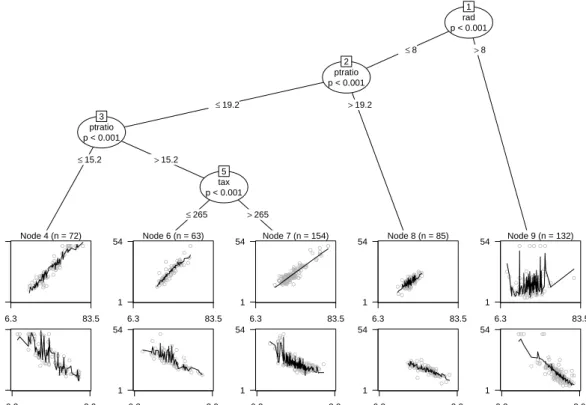
The resulting model-based tree is depicted in Figure1which shows partial scatter plots along with the fitted values in the terminal nodes. It can be seen that in the nodes 4, 6, 7 and 8 the increase of value with the number of rooms dominates the picture (upper panel) whereas in node 9 the decrease with the lower status population percentage (lower panel) is more pronounced. Splits are
rad p < 0.001 1 ≤8 >8 ptratio p < 0.001 2 ≤19.2 >19.2 ptratio p < 0.001 3 ≤15.2 >15.2 Node 4 (n = 72) ● ● ●●● ● ● ● ●● ●●● ●●● ● ● ●●●● ● ● ● ●● ● ● ● ●● ● ● ●● ● ● ● ● ● ● ● ● ● ● ● ● ● ● ●● ● ● ●● ● ● ● ● ● ● ● ● ● ● ● ●● ● ● ● 6.3 83.5 1 54 ● ● ● ● ● ●● ● ● ● ● ● ●●●● ● ● ● ● ● ● ● ● ●● ● ●● ● ● ● ● ● ●● ● ● ● ● ● ● ● ● ● ● ● ● ● ● ● ● ● ● ● ● ● ● ● ● ● ● ● ● ● ● ● ●● ● ● ● 0.3 3.9 1 54 tax p < 0.001 5 ≤265 >265 Node 6 (n = 63) ● ● ●● ●● ● ● ●● ● ●● ● ● ● ●● ● ● ● ● ●● ●● ●●● ●●● ● ● ● ● ● ● ●● ● ● ● ● ● ●●● ● ●●● ● ● ● ● ● ● ● ● ● ● ● 6.3 83.5 1 54 ● ● ● ● ● ● ● ●● ● ●● ●● ● ● ● ● ● ● ● ● ● ● ● ● ●● ● ● ● ● ● ●●● ● ● ● ● ● ● ● ● ● ● ●● ● ● ●●● ● ● ● ● ● ● ● ● ● ● 0.3 3.9 1 54 Node 7 (n = 154) ● ● ● ●● ●● ●● ●● ● ●●●● ● ● ●● ● ● ● ● ● ● ● ● ●● ● ● ● ● ● ● ● ● ●●● ●●● ● ● ●●● ● ●● ● ●● ● ● ●● ● ●●● ● ●●● ● ● ● ● ● ● ● ● ● ● ● ● ● ● ● ● ● ● ● ● ● ●●● ●●● ● ● ● ●●●● ● ● ● ● ● ● ● ●●● ● ● ● ● ● ● ● ● ● ● ● ● ●● ● ●●● ● ● ●●● ●● ● ● ● ● ● ● ●● ● ● ●● ● ● ●● ● ● 6.3 83.5 1 54 ● ●● ●● ● ● ● ● ● ● ● ● ● ●● ● ●●●● ● ● ●● ● ● ● ● ● ● ● ● ● ● ● ● ● ●● ●●● ●●●● ●● ● ● ● ● ● ● ●●●● ● ● ● ● ● ● ● ● ● ● ● ● ● ● ● ● ● ● ● ● ● ● ● ● ● ● ● ● ● ●●●●● ● ●● ● ● ● ● ● ● ● ● ● ● ● ● ●●●●● ●● ● ● ● ● ● ● ● ● ● ●● ●●● ●● ● ● ● ● ● ● ● ● ● ●● ● ● ● ● ● ● ● ● ● ● ● ● 0.3 3.9 1 54 Node 8 (n = 85) ● ● ●● ● ●● ● ● ● ●● ●●● ●● ● ●● ● ● ● ● ● ● ● ●● ●● ● ●● ● ●● ●●● ●● ● ● ● ● ● ●● ●● ● ● ● ● ● ● ● ● ● ● ● ●●● ● ● ●●●● ● ● ●● ● ● ● ● ●●●●● ● 6.3 83.5 1 54 ●●● ● ● ● ● ● ● ●● ● ● ●● ● ● ● ●●●● ● ● ● ● ● ●● ● ● ● ●● ●●● ●●● ● ● ● ● ● ● ● ● ● ● ● ● ● ● ● ● ● ●● ● ● ●●●●●●●●●● ● ● ● ● ● ● ● ● ● ● ● ●● ● 0.3 3.9 1 54 Node 9 (n = 132) ●● ● ●● ● ● ● ● ● ● ● ● ●●● ● ● ● ●●●● ●●● ● ● ●●● ●●● ● ● ● ● ● ●● ● ● ●●● ● ●● ● ● ● ● ● ● ● ● ● ●● ●● ●● ● ● ● ● ● ● ● ●●●● ● ● ● ● ● ● ● ● ● ● ● ● ● ● ●●● ●●●●● ● ● ● ● ● ● ● ● ● ●● ● ●●●● ● ●●● ● ●●● ● ● ● ● ●● ●● ●●● 6.3 83.5 1 54 ● ● ●● ● ● ● ● ● ● ● ● ●● ● ●● ●● ●● ●●●●●●● ● ● ● ● ● ● ● ● ● ●●●● ● ● ● ● ● ● ● ● ● ● ● ● ● ● ●● ● ● ● ●● ●● ● ● ● ● ● ● ● ●●●●● ● ● ●● ●● ● ● ● ● ● ● ● ● ● ●●●●●● ● ● ●● ● ● ● ● ● ● ● ●● ● ●●●●●● ● ● ● ● ● ● ● ● ● ● ● ● ●●● 0.3 3.9 1 54
Figure 1: Linear-regression-based tree for the Boston housing data. The plots in the leaves give partial scatter plots for (rm)2(upper panel) and log(lstat) (lower panel).
Achim Zeileis, Torsten Hothorn, Kurt Hornik 7
performed in the variables ‘rad’ (index of accessibility to radial highways), ‘ptratio’ (pupil-teacher ratio) and ‘tax’ (poperty-tax rate). The model has 5·3 regression coefficients after estimating 5−1 splits, giving a total of 19 estimated parameters; the associated residual sum of squares is Ψ(Y,θˆ) = 6081.28, corresponding to a mean squared error of 12.02.
5. Further remarks and conclusion
A powerful, flexible and unified framework for model-based recursive partitioning has been sug-gested. It builds on parametric models which are well-established in the statistical theory and whose parameters can be easily interpreted by subject-matter scientists. Thus, it can not only model the mean but also other moments of a parameterized distribution (such as variance or cor-relation). Furthermore, it can be employed to partition regression relationships, such as GLMs or survival regression. It aims at minimizing a clearly defined objective function (and not certain heuristics) by a greedy forward search and is unbiased due to separation of variable and cutpoint selection.
The algorithm as discussed in this paper relies on a statistically motivated internal stopping criterion (sometimes called pre-pruning), but, of course, it could also be combined with cross-validation-based post-pruning although the statistical interpretation of thep values would then be lost. As every node of the tree is associated with a fitted model with a certain number of parameters, another attractive option is to grow the tree with a largeαand then prune based on information criteria.
For some statistical models, there is a clearly defined estimating function ψ(Y, θ) but the an-tiderivate Ψ(Y, θ) does not necessarily exist. Such models can also be recursively partitioned: the parameter instability tests work in the same way, only the selection of the splits has to be adapted. Instead of minimizing an objective function, the correspondingB-sample split statistics have to be maximized.
Typically, recursive partitioning algorithms use perpendicular splits, i.e., the partitioning variables
Zj just include ‘main effects’. To prevent that the algorithm fails to pick up ‘interaction effects’ such as the XOR problem, interactions could also be added to the list of partitioning variables. If regression models are partitioned, the question arises whether a certain covariate should be included in Y as a regressor or in Z as a partitioning variable. For categorical variables, this amounts to knowing/assuming the interactions or trying to find them adaptively—for numerical variables, it amounts to knowing/assuming a segment-wise linear relationship vs. approximating a possibly non-linear influence by a step function. The separation can usually be made based on subject knowledge: e.g., in biostatistics it would be natural to fit a dose-response relationship and partition it with respect to further experiment-specific covariables, or in business applications a market segmentation could be carried out based on a standard demand function. Finally, the variables entering the explanatory part of Y and Z could also be overlapping, but then a trend-resistant fluctuation test should be conducted during partitioning.
Within the genuine statistical framework proposed in this paper, practitioners can assess whether one (standard) global parametric model fits their data or whether it is more appropriate to par-tition it with respect to further covariates. If so, the parpar-titioning variables and their split points are selected separately in a forward search that controls the type I error rates for the variable selection in each node. This formulation of the algorithm ensures that interpretations obtained from graphical representations of the corresponding tree-structured models are valid in a statistical sense.
References
Andrews DWK (1993). “Tests for Parameter Instability and Structural Change With Unknown Change Point.”Econometrica,61, 821–856.
Andrews DWK, Ploberger W (1994). “Optimal Tests When a Nuisance Parameter is Present Only Under the Alternative.”Econometrica,62, 1383–1414.
Bai J, Perron P (2003). “Computation and Analysis of Multiple Structural Change Models.”
Journal of Applied Econometrics,18, 1–22.
Breiman L (2001). “Random Forests.”Machine Learning, 45(1), 5–32.
Breiman L, Friedman JH (1985). “Estimating Optimal Transformations for Multiple Regression and Correlation.”Journal of the American Statistical Association,80(391), 580–598.
B¨uhlmann P, Yu B (2003). “Boosting withL2Loss: Regression and Classification.”Journal of the
American Statistical Association,98(462), 324–338.
Chan KY, Loh WY (2004). “LOTUS: An Algorithm for Building Accurate and Comprehensible Logistic Regression Trees.”Journal of Computational and Graphical Statistics,13(4), 826–852. Choi Y, Ahn H, Chen JJ (2005). “Regression Trees for Analysis of Count Data With Extra Poisson
Variation.”Computational Statistics & Data Analysis,49, 893–915.
Chu CSJ, Hornik K, Kuan CM (1995). “MOSUM Tests for Parameter Constancy.” Biometrika,
82, 603–617.
Gama J (2004). “Functional Trees.”Machine Learning,55, 219–250.
Hawkins DM (2001). “Fitting Multiple Change-Point Models to Data.”Computational Statistics & Data Analysis,37, 323–341.
Hjort NL, Koning A (2002). “Tests for Constancy of Model Parameters Over Time.”Nonparametric Statistics,14, 113–132.
Kim H, Loh WY (2001). “Classification Trees With Unbiased Multiway Splits.” Journal of the American Statistical Association,96(454), 589–604.
Loh WY (2002). “Regression Trees With Unbiased Variable Selection and Interaction Detection.”
Statistica Sinica,12, 361–386.
Meyer D, Leisch F, Hornik K (2003). “The Support Vector Machine Under Test.”Neurocomputing,
55(1–2), 169–186.
Morgan JN, Sonquist JA (1963). “Problems in the Analysis of Survey Data, and a Proposal.”
Journal of the American Statistical Association,58, 415–434.
Muggeo VMR (2003). “Estimating Regression Models With Unknown Break-Points.”Statistics in Medicine,22, 3055–3071.
Nyblom J (1989). “Testing for the Constancy of Parameters Over Time.”Journal of the American Statistical Association,84, 223–230.
O’Brien SM (2004). “Cutpoint Selection for Categorizing a Continuous Predictor.” Biometrics,
60, 504–509.
Ploberger W, Kr¨amer W (1992). “The CUSUM Test With OLS Residuals.”Econometrica,60(2), 271–285.
Achim Zeileis, Torsten Hothorn, Kurt Hornik 9
Quinlan JR (1993).C4.5: Programs for Machine Learning. Morgan Kaufmann Publ., San Mateo, California.
Samarov A, Spokoiny V, Vial C (2005). “Component Indentification and Estimation in Nonlin-ear High-Dimension Regression Models by Structural Adaptation.” Journal of the American Statistical Association,100(470), 429–445.
Su X, Wang M, Fan J (2004). “Maximum Likelihood Regression Trees.”Journal of Computational and Graphical Statistics,13, 586–598.
Vapnik VN (1996). The Nature of Statistical Learning Theory. Springer, New York.
White H (1994). Estimation, Inference and Specification Analysis. Cambridge University Press. Zeileis A (2005). “A Unified Approach to Structural Change Tests Based on F Statistics, OLS
Residuals, and ML Scores.”Report 13, Department of Statistics and Mathematics, Wirtschaft-suniversit¨at Wien, Research Report Series. URLhttp://epub.wu-wien.ac.at/.
Zeileis A, Hornik K (2003). “Generalized M-Fluctuation Tests for Parameter Instability.”Report 80, SFB “Adaptive Information Systems and Modelling in Economics and Management Science”.
URLhttp://www.wu-wien.ac.at/am/reports.htm#80.
Zeileis A, Kleiber C, Kr¨amer W, Hornik K (2003). “Testing and Dating of Structural Changes in Practice.”Computational Statistics & Data Analysis, 44(1–2), 109–123.