University of Kentucky
UKnowledge
Biostatistics Faculty Publications
Biostatistics
4-2016
Uncovering Local Trends in Genetic Effects of
Multiple Phenotypes via Functional Linear Models
Olga A. Vsevolozhskaya
University of Kentucky, [email protected]
Dmitri V. Zaykin
National Institute of Environmental Health Sciences
David A. Barondess
Michigan State University
Xiaoren Tong
Michigan State University
Sneha Jadhav
Michigan State University
See next page for additional authors
Right click to open a feedback form in a new tab to let us know how this document benefits you.
Follow this and additional works at:
https://uknowledge.uky.edu/biostatistics_facpub
Part of the
Biostatistics Commons
,
Environmental Public Health Commons
, and the
Epidemiology Commons
This Article is brought to you for free and open access by the Biostatistics at UKnowledge. It has been accepted for inclusion in Biostatistics Faculty Publications by an authorized administrator of UKnowledge. For more information, please [email protected].
Repository Citation
Vsevolozhskaya, Olga A.; Zaykin, Dmitri V.; Barondess, David A.; Tong, Xiaoren; Jadhav, Sneha; and Lu, Qing, "Uncovering Local Trends in Genetic Effects of Multiple Phenotypes via Functional Linear Models" (2016).Biostatistics Faculty Publications. 32.
Authors
Olga A. Vsevolozhskaya, Dmitri V. Zaykin, David A. Barondess, Xiaoren Tong, Sneha Jadhav, and Qing Lu
Uncovering Local Trends in Genetic Effects of Multiple Phenotypes via Functional Linear ModelsNotes/Citation Information
Published in
Genetic Epidemiology
, v. 40, issue 3, p. 210-221.
Published 2016. This article is a U.S. Government work and is in the public domain in the USA.
Digital Object Identifier (DOI)https://doi.org/10.1002/gepi.21955
Genetic
Epidemiology
R
ESEARCH
A
RTICLE
Uncovering Local Trends in Genetic Effects of
Multiple Phenotypes via Functional Linear Models
Olga A. Vsevolozhskaya,1†∗Dmitri V. Zaykin,2†David A. Barondess,3Xiaoren Tong,3Sneha Jadhav,4and Qing Lu3
1Department of Biostatistics, University of Kentucky, Lexington, Kentucky, United States of America;2National Institute of Environmental Health Sciences, National Institutes of Health, Bethesda, Maryland, Research Triangle Park, North Carolina, United States of America;3Department of Epidemiology and Biostatistics, Michigan State University, East Lansing, Michigan, United States of America;4Department of Statistics, Michigan State University, East Lansing, Michigan, United States of America
Received 7 September 2015; Revised 4 December 2015; accepted revised manuscript 14 December 2015. Published online 29 March 2016 in Wiley Online Library (wileyonlinelibrary.com). DOI 10.1002/gepi.21955
ABSTRACT: Recent technological advances equipped researchers with capabilities that go beyond traditional genotyping of loci known to be polymorphic in a general population. Genetic sequences of study participants can now be assessed directly. This capability removed technology-driven bias toward scoring predominantly common polymorphisms and let researchers reveal a wealth of rare and sample-specific variants. Although the relative contributions of rare and common polymorphisms to trait variation are being debated, researchers are faced with the need for new statistical tools for simultaneous evaluation of all variants within a region. Several research groups demonstrated flexibility and good statistical power of the functional linear model approach. In this work we extend previous developments to allow inclusion of multiple traits and adjustment for additional covariates. Our functional approach is unique in that it provides a nuanced depiction of effects and interactions for the variables in the model by representing them as curves varying over a genetic region. We demonstrate flexibility and competitive power of our approach by contrasting its performance with commonly used statistical tools and illustrate its potential for discovery and characterization of genetic architecture of complex traits using sequencing data from the Dallas Heart Study.
Genet Epidemiol 40:210–221, 2016.©2016 Wiley Periodicals, Inc.
KEY WORDS:multivariate analysis; pleiotropy; genome-wide association studies; sequencing studies; quantitative traits; qual-itative traits; functional analysis
Introduction
Genome-wide association studies (GWAS) have identified numerous risk loci for common complex diseases, and next-generation sequencing based association strategies are now emerging to characterize the contribution of rare genetic variants to human genetic disorders. Analysis of the “rare variant—common complex disease” hypothesis requires tai-lored statistical methods, as single marker tests fail to uncover these rare variants [Carvajal-Carmona, 2010]. An entirely new powerful class of statistical methods based on nonpara-metric functions was recently developed for genetic asso-ciation testing that can accommodate both rare and com-mon variants, or the combination of the two [Fan et al., 2013, 2014; Lee et al., 2014; Luo et al., 2011, 2012a, b; Svishcheva et al., 2015; Vsevolozhskaya et al., 2014; Wang et al., 2015; Zhu and Xiong, 2012]. A comprehensive com-parison of nonparametric functional-based methods (FBMs) via simulation studies and real data applications have re-peatedly shown that FBMs have a valid type I error rate
†These authors contributed equally to this work.
∗Correspondence to: Olga A. Vsevolozhskaya, Department of Biostatistics, College
of Public Health, University of Kentucky, 725 Rose Street, Lexington, KY 40536-0082. E-mail: [email protected]
and a substantially higher power to detect an association compared with alternative approaches. Additionally, FBMs were proven to be a powerful approach for genetic associa-tion studies with longitudinal data [Reimherr et al., 2014], or for the analysis of gene expression data [Storey et al., 2005].
Recently, our research group has demonstrated that within FBMs, functional analysis of variance (FANOVA) attains higher power to detect an association between a genetic re-gion and a dichotomous trait compared to methods based on functional linear models (FLMs) [Vsevolozhskaya et al., 2014]. Specifically, we have shown that FANOVA outper-forms FLM for small to moderate effect sizes of the variants within a genetic region. Nonetheless, from a practical point of view, FANOVA had a notable limitation in that it was not able to accommodate quantitative traits or adjust for continuous covariates.
In light of these shortcomings, our aim was to extend the existing FANOVA method to association analyses of multiple quantitative and qualitative traits and to accommodate situa-tions in which (1) a gene influences more than one trait (i.e., pleiotropy), (2) where there are confounding/mediation ef-fects (due to population substructure or other sources), and (3) where the effect of disease risk can be modified by a
trait or an exposure—a phenomena that we refer hereafter as ‘treatment by trait” (T×T) interaction.
To conceptualize T×T interaction, consider a study of ge-netic risk factors of substance abuse disorder. It is well known that personality traits such as impulsivity and sensation seek-ing are highly prevalent in drug-dependent individuals [e.g., De Wit, 2009]. It is also known that personality traits are sub-stantially influenced by genes [e.g., Bouchard Jr and Loehlin, 2001]. Suppose there are genetic risk factors that contribute to the increased risk of developing drug addiction among individuals with high trait impulsivity. Suppose, further, that a different genetic disposition might be involved in the in-creased risk of developing drug addiction among individuals with low trait impulsively. Hence, risk alleles for drug depen-dence (i.e., “treatment”) might vary by the level of personality traits, which will be modeled as T×T interaction in our gen-eralized FANOVA approach—more on this later.
A distinctive contribution of the approach presented here to the emerging field of FBMs for genetic association studies is the introduction of an efficient way to estimate the effects of phenotypes, confounding factors, and T×T interactions using continuous curves smoothly varying over genetic loci. Previously proposed functional methods for genetic associ-ation studies [e.g., Fan et al., 2013; Luo et al., 2011, 2012a] and other methods that combine information across multi-ple variants within a gene [e.g., Liu and Leal, 2010; Wu et al., 2011] aggregate across both the association signals of genetic variants as well as over covariate effects. We exploit the flex-ibility of the functional approach to unveil a more nuanced blueprint of how covariate and interaction effects vary within a genetic region by estimating partial regression coefficient curves that change over variant positions.
Unlike traditional statistical models that treat a disease phenotype as an outcome (i.e., on the left-hand side of the equation), our model puts nongenetic variables on the right-hand side, including traits, environmental exposures, and confounders. The response function in our model is an al-lelic dosage curve, fitted through genetic variants within a region. If we start our modeling by including a binary trait such as drug dependence as a single predictor, the continuous regression coefficient will be the difference between average allelic dosages over multiple variants of the two groups. That is, a continuous intercept curve will estimate smoothed aver-age allelic dosaver-age among nondrug-dependent controls, and a continuous regression coefficient will estimate a deviation from this baseline allelic dosage over multiple variants among drug-dependent cases. Further, if we include personality trait as a covariate, the regression coefficient curve for drug ad-diction will be adjusted for personality trait. Finally, if we include a T×T interaction between drug-dependence status and a personality trait, the deviation from the baseline allelic dosage among drug-dependent cases will vary by the level of a personality trait.
Functional models where genetic predictor (X) and the outcome (Y) are swapped in the regression equation are rem-iniscent of the reverse regression approach [Maddala, 1992]. In general, coefficients of the direct and the reverse
regres-sions are not the same, however the test statistic for theX
(adjusted for any covariates) as well as the corresponding par-tial correlation coefficient remain the same after the swap-ping. For example, adjustment for confounding or media-tion is unaffected and remains valid in the reverse regression approach.
To estimate continuous coefficient curves, our new gener-alized FANOVA approach utilizes a connection between pe-nalized spline regression and best linear unbiased predictors (BLUPs), enabling a straightforward practical implementa-tion using standard linear mixed models statistical software. A connection between BLUPs and penalized functional regres-sion has been explored in statistical and machine learning literature [Brumback et al., 1999; Crainiceanu et al., 2005; Crainiceanu and Goldsmith, 2010; Eilers and Marx, 1996; Goldsmith et al., 2010; Ivanescu et al., 2015; Lian, 2007; Nosedal-Sanchez et al., 2012; Pearce and Wand, 2006; Rup-pert et al., 2003; Wand and Ormerod, 2008; Wang, 1998]. However, this connection has largely been ignored in func-tional method approaches for genetic association studies.
We provide an illustration of our method using data from the Dallas Heart Study [Romeo et al., 2007], by characteriz-ing associations of sequence variants with plasma triglyceride (TG) levels, modified by race and adjusted for sex. In addition to identifying the originally reported association between TG levels and theANGPTL4gene, our new FANOVA approach identified specific subregions of the ANGPTL4gene asso-ciated with plasma TG levels among European Americans, African Americans, and Hispanics.
Methods
Genotypic Functions: A Brief Overview
In brief, our method is an extension of the previously pro-posed FANOVA methodology, which seeks to quantify the relationship between scalar phenotypesX1,X2, . . . ,Xkand smooth genotypic functionsG(t)’s, withtindexing a genetic variant’s position over a genetic region,t∈[0, τ] [Vsevolozh-skaya et al., 2014]. By using the term “genotypic functions,” we refer to nonparametric functions fitted with a basis expan-sion method [Ramsay and Silverman, 2005; Ruppert et al., 2003; Wood, 2006]. Thus, for each subject, the genetic data is not of a discrete (i.e., counted) nature, such as would be the case for genotype frequencies, but rather a single nonpara-metric genotypic function,G(t), of a continuous nature.
A genotypic function is obtained by either (i) a cubic B-spline basis expansion over a dense set of knots,κ1, . . . , κK, over the range of the variant’s genomic positionsti’s (in the one-base coordinate system) or (ii) penalized spline smooth-ing that avoids the knot selection problem completely [e.g., Luo et al., 2012a, Vsevolozhskaya et al., 2014]. Earlier in-vestigations of FLMs designed for genetic association testing include comprehensive coverage of the estimation procedure for the genotypic functionsG(t)’s [Fan et al., 2013, 2014; Lee et al., 2014; Luo et al., 2011, 2012a, b; Svishcheva et al.,
2015; Vsevolozhskaya et al., 2014; Wang et al., 2015; Zhu and Xiong, 2012].
If we letG1(t), . . . ,GN(t),t∈[0, τ] denote the functional genotypic data forNindividuals, and we letX1i, . . . ,XPi,i= 1, . . . ,Ndenote a set ofPvariables that consists of covariates and traits (either quantitative or qualitative) that may con-tribute to a disease, our model for each individual’s genotypic function is:
Gi(t)=β0(t)+β1(t)X1i+· · ·+βP(t)XPi+i(t), (1)
whereβi(t)’s are continuous regression coefficients that de-scribe an association between a scalar trait and a set of vari-ants in a genetic regiont∈[0, τ], and where(t) is a residual function. Unlike traditional models where the outcome is re-gressed on a set of predictors, this model treats genetic infor-mation as an outcome. Outside of the functional approach, utility of such “reverse regressions” has been explored previ-ously for analysis of genetic associations [Feng, 2014; Kwan et al., 2011]. Although coefficient estimates change, in gen-eral, due to swapping of variables between two sides of a regression equation, the partial correlations as well as the test statistics andP-values for the coefficients remain invariant: this follows simply from expressing these quantities in terms of the entries of the inverse of the correlation matrix between all variables including the outcome. Thus, testing for effects or for validity of regression adjustments are preserved under the reversal. There is also convenience in having the same type of outcome (i.e., genetic information) and thus the same type of a link function regardless of the type and the number of other variables in the model. Additionally, within the func-tional approach, exploration of ˆβ(t)’s may allow researchers to determine subregions of [0, τ] that harbor causal genetic variants (i.e., subregions over which ˆβ(t)=0).
To estimate ˆβ(t)’s, we place a function-on-scalar regression in Equation(1) into the context of a mixed-effects model or, more generally, embed the penalized splines problem into the class of reproducing kernel methods. To introduce the method, we first present a case of a single curve estimation, and conclude with the general case that allows us to estimate continuous coefficients of multiple traits, construct their con-fidence intervals, and test for an association. We finally note that in the context of this paper, the word “kernel” should not be confused with a weight function as in the local regression (or local smoothing), which is also called a kernel [Hastie et al., 2009].
Estimating a Single Curve
To draw connections between smoothing splines and re-producing kernels, first consider a simpler problem of es-timating a single curve from the observed yi’s and ti’s,
i=1, . . . ,n. One possible approach to estimating a nonpara-metric functionf(t) from discrete data is to invoke penalized spline smoothing [e.g., Wahba, 1990]. This smooth interpo-lation of the data is achieved by minimizing least squares fits
with an additional roughness penalty (i.e., penalized sums of squares) as follows: min n–1 n i=1 (yi–f(ti))2+λ 1 0 [L y(t)]2dt . (2) Here, the roughness of a function is quantified by the square of a linear differential operator L y(t) (a typical choice is
L y(t)=f(t) that corresponds to penalizing curvature of the function). The constant term,λ, referred to as a smoothing or a tuning parameter, should be either specified by a user or determined through the generalized cross-validation (GCV) [Wood, 2006].
The above minimization problem is analogous to a corre-sponding regularization problem within the machine learn-ing domain: min f∈H n i=1 L(yi,f (ti))+λPf2H , (3)
whereL(yi,f (ti)) is a loss function,Pf2 penalizes f in terms of the variability of its function values, andHis the reproducing kernel Hilbert space (RKHS) of real functions
f . The theory of RKHS was developed by Aronszajn [1950] and Saitoh [1988], with good overviews provided by Wahba [1990], Smola and Sch¨olkopf [1998], and Rasmussen and Williams [2006]. Briefly, a RKHS onRd is a Hilbert space of real-valued functions generated by a bivariate symmetric, positive definite kernelk(·,·) with the following properties: (i) for everytinRd,k(t,t) is a function oftinHand (ii)
khas the reproducing propertyk(·,ti),f H=f(ti), where ·,·denotes the inner product. To conceptualize penalized splines in Equation (2) as BLUPs in a mixed model frame-work, we explore the solution to the regularization problem in Equation (3) from the machine learning theory. Based on the results of therepresenter theorem[Kimeldorf and Wahba, 1971], it can be shown that each minimizerf ∈Hof Equa-tion (3) can be written as a linear combinaEqua-tion of kernel functions, as follows: f (t)= n i=1 αik(t,ti). (4) The solution for α=[α1, . . . , αn] can be obtained as ˆα= (K+λIn)–1y, in whichKis the n×n matrix with theijth entry ofk(ti,tj),Iis then×nidentity matrix, andyis the
n×1 vector of observedyi’s [Hastie et al., 2009; Rasmussen and Williams, 2006]. Further, the vector of nfitted values is given by ˆf=Kαˆ. This solution looks very similar to that from a linear regression model (i.e., ˆy=Tβˆbecause we usedti insteadxiin Eqs. (2–3)). Regrettably, this reproducing kernel transformation ofti’s does not simply move our nonlinear problem into the “friendly” linear model domain, because the solution forαdepends onλ.
A slight variation to therepresenter theoremcan be achieved by decomposing H into H0⊕H1, where H0 is a
finite-dimensional null space containing terms that will not be penalized, andH1is its orthogonal complement (i.e.,
penal-ized terms). For example, forPf2defined by differential
operators of the formL y(t)=f (m)(t), the null spaceH 0 is
spanned by polynomials of degree up tom–1. More specif-ically, ifm=2, then constant and linear functions are in the null space, because they are not penalized for “curvature.” With the decomposition ofH, the minimizerf of the regu-larization function in Equation (3) now has the form:
f(t)= m j=1 djφj(t)+ n i=1 cik1(t,ti), (5) where φ1(t), . . . , φm(t) form the basis ofH0 andk1(·,·) is
a reproducing kernel that generates H1. If m=2 as in the
example above, then φ1(t)=1 and φ2(t)=t span the null
space of unpenalized functions.
There are relatively few published recommendations in the statistical literature on how to constructk1(·,·). For example,
Lian [2007] writes “[...]the construction ofk1 in general is
difficult and a search of the literature does not seem to provide us with any clues about how to construct a positive definite kernel in general.” Nonetheless, if we shift our attention to the machine learning literature, we see thatk1(t,ti)=G(t,ti), whereG(t,ti) is a Green’s function of the linear differential operator L y(t) [Fasshauer, 2012; Fasshauer and Ye, 2013; Poggio and Girosi, 1990; Rasmussen and Williams, 2006]. Note that the Green’s function also depends on the bound-ary conditions. A “natural” choice is the ‘natural boundbound-ary condition”f(j)(a)=f (j)(b)=0, j =1, . . . ,m; whereaand
b are the boundaries of the functional domain [Green and Silverman, 1993].
How can we estimate the fitted values of the coefficients ˆd
and ˆcin Equation (5) for a specific problem? If we rewrite Equation (5) using linear algebra notations as:
ˆ
f=dˆ+K1ˆc, (6)
it becomes evident that Equation (6) represents a solution to the linear mixed-effects model with design matricesand
K1, and ˆdand ˆcestimated as BLUPs from this model [Speed,
1991]. In addition, the BLUP solution for the coefficients is independent of the smoothing parametersλ, which is equal to the ratio of the variances of the residuals and random ef-fects. For numerical stability reasons, the design matrices are specified for a sequence of knotsk1, . . . ,kκplaces at sample
quantilies over the range ofti’s [Ruppert, 2002] as:
= ⎡ ⎢ ⎣ 1 t1 .. . ... 1 tn ⎤ ⎥ ⎦ and K1= ⎡ ⎢ ⎣ (t1–k1)+ · · · (t1–kκ)+ .. . . .. ... (tn–k1)+ · · · (tn–kκ)+ ⎤ ⎥ ⎦, (7) whereG(ti,tj)=(ti–tj)+is the Green’s function of the linear
differential operatorf(2)(t), andx
+=max{0,x}. This
specifi-cation of the design matrices corresponds to a truncated lines series basis expansion ˆf (t)=dˆ0+dˆ1t+
κ
i=1cˆi(t–ki)+. Other
choices of basis functions can also be used with correspond-ing changes to penalized terms. Possible choices include, but are not limited to, (a) truncated power basis (t–ki)p+, (b)
O’Sullivan splines [Wand and Ormerod, 2008], (c) thin plate
splines [Ivanescu et al., 2015], or (d) the Gaussian kernel [Lian, 2007].
Some readers might wonder whether the mixed model for-mulation for penalized splines bear the same parameter in-terpretation as in a typical application to nested hierarchical data. We should clarify that the functional representation in Equation (6) is just a convenient way of shifting a nonlinear problem into a linear domain, while simultaneously estimat-ing a smoothestimat-ing parameter. Similarly, the random effects in
care just a convenience device to model the curvature inf
and should not be interpreted as random effects, per se. Estimatingβ(t)’s
With respect to the conceptual model in Equation (1), continuous regression coefficients can be estimated as fol-lows. For each subject, the genotypic function is evalu-ated on the grid of genomic positionst1, . . . ,tn, i.e, ˆGi(t)=
ˆ
Gi(t1), . . . ,Gˆi(tn). For the sequence of knotsk1, . . . ,kκ, each
functional regression coefficient is expanded in terms of the linear combination ofφ’s andk1’s. This expansion yields the
following mixed-model representation of Equation (1): ˆ Gi(t)=βˆ0(t)+βˆ1(t)X1i+· · ·+βˆP(t)XPi (8) =( ˆd1+dˆ2t+ κ i=1 k1(t,ki)ˆci) ˆ β0(t) +( ˆd∗1+dˆ∗2t+ κ i=1 k1(t,ki)ˆc∗i) ˆ β1(t) X1i+· · · +( ˆd1+dˆ2t+ κ i=1 k(t,ki) ˆci) ˆ βP(t) XPi.
Conceptually, the generalized FANOVA-based regression coefficients, β(t)’s, are similar to the genetic effect coeffi-cients in the recently published paper by Wang et al. [2015]. Specifically, Wang et al. [2015] also proposed to estimate regression coefficients,βl(t)’s, smoothly varying over the ge-netic positiont. However, unlike the methodology proposed in the present study, their approach cannot simultaneously handle quantitative and qualitative traits, adjust coefficients for confounders/mediators over a continuum [0, τ], or mod-ify effects by the level of another trait. With our approach, this adjustment can be easily incorporated into the model.
Suppose we want to adjust the effect of a risk factorX1by
traitX2overallt. The model will be written as:
ˆ
Gi(t)=βˆ0(t)+βˆ1(t)X1i+βˆ2(t)X2i.
Suppose, further, we want to modify the effect of a risk factor
simplicity, assume thatX2has only two levels). The model
can be expressed as: ˆ
Gi(t)=βˆ0(t)+βˆ1(t)X1i+βˆ2(t)X2i+βˆ12(t)X1iX2i. Then, for the first level ofX2, dummy coded as 0, the
associ-ation between a gene andX1will be estimated by ˆβ1(t):
ˆ
Gi(t)=βˆ0(t)+βˆ1(t)X1i,
and for the second level ofX2, dummy coded as 1, the
asso-ciation between a gene andX1will be modified as:
ˆ
Gi(t)=( ˆβ0(t)+βˆ2(t))+( ˆβ1(t)+βˆ12(t))X1i. To facilitate the data analysis using mixed-effects software, an input response should be a vectorized matrix of genotype functions for N subjects eval-uated on the grid of genomic positions, vec( ˆG)= [ ˆG1(t1), . . . ,Gˆ1(tn), . . . ,GˆN(t1), . . . ,GˆN(tn)]. Input pre-dictors should beN·n×1 vectorsX1, . . . ,XP, which are generated by repeating each phenotype observationntimes and stacking them on top of one another. The fixed- and the random-effects design matrices,andK1, are then
con-structed as follows: = ⎡ ⎢ ⎢ ⎢ ⎢ ⎢ ⎢ ⎢ ⎢ ⎢ ⎢ ⎢ ⎣ 1 t1 X11 t1X11 · · · XP1 t1XP1 . . . . . . . . . . . . . .. ... . . . 1 tn X11 tnX11 · · · XP1 tnXP1 . . . . . . . . . . . . . .. ... . . . 1 t1 X1N t1X1N · · · XPN t1XPN . . . . . . . . . . . . . .. ... . . . 1 tn X1N tnX1N · · · XPN tnXPN ⎤ ⎥ ⎥ ⎥ ⎥ ⎥ ⎥ ⎥ ⎥ ⎥ ⎥ ⎥ ⎦ = ⎡ ⎢ ⎣1N⊗ ⎡ ⎢ ⎣ 1 t1 . . . . . . 1 tn ⎤ ⎥ ⎦,X1⊗ ⎡ ⎢ ⎣ 1 t1 . . . . . . 1 tn ⎤ ⎥ ⎦, . . . ,XP⊗ ⎡ ⎢ ⎣ 1 t1 . . . . . . 1 tn ⎤ ⎥ ⎦ ⎤ ⎥ ⎦, and K1=[1N⊗K, X1⊗K, . . . ,XP⊗K], where 1N is
N×1 vector of 1’s,⊗is the Kronecker product, and Kis then×κmatrix with theijth entry ofk1(ti,kj) calculated over the sequence of knotsk1, . . . ,kκ.
Confidence Interval for ˆβ(t)
Because the conceptual model in Equation (1) can be ex-pressed as a mixed-effects model in Equation (8), the typical inferential machinery for mixed-effects models can be used to obtain the variance-covariance estimates of the model pa-rameters [Ruppert et al., 2003]. An explicit formulation for the estimated standard deviation of ˆβ(t) is:
st.dev( ˆβ(t))=σˆ
C(CC+λˆD)–1CC(CC+λˆD)–1C, (9) where ˆσ is a REML estimate ofσ,C=[K1] is formed
by two design matrices described in Equation (7), ˆλ=σˆ2/σˆc2
is the estimated smoothing parameter, andD is formed as follows: D= 0m×m 0m×κ 0κ×m Iκ×κ ,
where m is the number of “fixed effects” and κ is the number of “random effects.” An approximate pointwise 100%(1–α) confidence interval is ˆβ(t)±z(1–α/2)st.dev( ˆ β(t)).
Alternatively, Bayesian credible intervals can be obtained by realizing a connection between Gaussian processes and spline construction [Crainiceanu et al., 2005; Rasmussen and Williams, 2006], or “subject re-sampling” bootstrap error bars can be obtained to construct the confidence intervals [Wu and Yu, 2002].
In the application of pointwise bands to functional geno-type data, the issue of bias-variance trade-off associated with the selection of the degree of smoothing might deserve more careful attention. Specifically, in the context of the mixed-effects model in Equation (8), the response variable is a fitted genotypic function ˆG(t). If the fitted function is somewhat wiggly, this “noise” will account for the increased width of the pointwise standard error bands for ˆβ(t). We previously proposed the “flipping algorithm” for genotype relabeling that decreases the number of noisy oscillations for smoothed genotype data and showed that this approach results in a substantial increase of statistical power to detect a genetic association [Vsevolozhskaya et al., 2014]. Nonetheless, too smooth genotype functions might result in narrow standard error bands for ˆβ(t) and thus estimate a biased version of a true function with great reliability. Further research is needed on the issue of optimal choice of a smoothing parameter in the context of genotype function fitting.
Testing for an Association
In this section we turn our attention to a test statistic used for evaluating an association between a genetic region and one or more phenotypes. Whereas different types of point-wise confidence intervals for the coefficient curves can be constructed, the hypothesis testing problem of distinguish-ing an optimal submodel ofβ(t)’s is still of interest. To ad-dress this issue, we will use the functionFstatistic [Shen and Faraway, 2004] as previously used in our FANOVA method-ology [Vsevolozhskaya et al., 2014]. Specifically, suppose we want to test the nullity of a single predictor:
H0:βi(t)=0, i=1, . . . ,P.
By using Theorem 2 in Shen and Faraway [2004], a test statis-tic to determine ifβ(t) is equivalent to the zero function can be constructed as follows: F= (N –P)βˆ2 i(t)dt rss1(XX)–ii1 , (10)
where X=(1 X1 . . . XP) is a design matrix for the full model containing all phenotypic variables, and rss1= N
i=1
( ˆGi(t)–Xβˆ)2dtis the residual sum of squares for the full model. Under the null hypothesis, it can be easily shown
214
Genetic Epidemiology, Vol. 40, No. 3, 210–221, 2016[e.g., Reimherr et al., 2014; Shen and Faraway, 2004; Zhang, 2013] that the distribution ofFcan be approximated by an
F-distribution as: F∼Fdˆ,(N–P) ˆd, where ˆd= ( n i=1ri)2 n
i=1r2i , withnbeing the number of genetic vari-ants, and ri is the ith order eigenvalue of the empirical variance-covariance matrix under the full model, ˆ1.
Alternatively, if we want to test the nullity ofK predictors simultaneously, that is, to compare the full model:
ˆ Gi(t)= P j=1 ˆ βj(t)Xij, to the reduced model:
ˆ Gi(t)= (P–K) j=1 ˆ βj(t)Xij,
the test statisticFcan be defined in terms of the reduction in the sums of squared errors, as follows:
F= (rss0
–rss1)/K
rss1/(N–P)
≈ trace( ˆ0–ˆ1)/K
trace( ˆ1)/(N–P), (11)
where rss0 is the residual sum of squares for the reduced
model, and ˆ0is the empirical variance-covariance matrix
under the reduced model. Under the null hypothesis, the distribution ofFis approximated byFKdˆ,(N–P) ˆd.
We note that the test statistic in Equation (11) is computa-tionally more complex than the one in Equation (10). That is, if the goal is to test the nullity of only one predictor at a time, the test statistic in Equation (10) can be calculated directly by fitting only the full model, and thus omitting fitting the reduced model. Further details and comparisons of the two formulas can be found in Shen and Faraway [2004].
Simulation Study
Design
The flexibility of our method allows us to accommodate various analysis settings and types of variables, including multiple, possibly correlated or pleiotropic phenotypes, and T×T interactions. One way to analyzing multiple traits is to test for an association one trait at a time. For a proper control of the experiment-wise false-discovery error rate, this “one at a time” testing approach requires accounting for the number of tests performed and correcting for each individual trait’sP -value. This individual correction typically leads to an inflation in the observedP-values. However, our method provides an efficient way of testing multiple traits simultaneously, with noP-value correction required, and thus naturally provides superior performance in terms of statistical power to detect an association. Moreover, to handle T×T interactions, or to assess modification of genetic susceptibility to disease by trait, our model requires a test of nullity for an interaction term. Previously, we investigated the power of FANOVA to detect an association with a single predictor [Vsevolozhskaya
Figure 1. The genetic information (G(t)) is directly associated with the outcome of interest (X) and indirectly through the third variable (Z).
et al., 2014]. Simulation studies presented here reflect the extension of our previous basic model with the addition of mediation/confounding scenarios.
Figure 1 aids in conceptualization of our data simula-tion process. We focused on a three variable system and hypothesized that there is a genetic predisposition (G) to continuous phenotypes (Z) and (X). We also assumed a relationship between (Z) and (X) and were interested in testing for an association between (G) and (X), while ad-justing for the third variable (Z). Clearly, data generated under this scenario fits the mediation analysis framework, but MacKinnon et al. [2000] point out that the label of (Z) (i.e., either as a mediator or a confounder) depends on the framework used to conceptualize the phenomenon. From a statistical modeling point of view, directionality and the causality are indistinguishable, making these seemingly dif-ferent concepts of mediation and confounding statistically equivalent. Therefore, data generated under our design can be used to check for both a mediator and a confounding control.
Data Generation
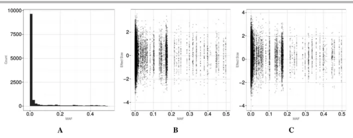
We generated genetic data (G) using the 1000 genome project [Durbin et al., 2010] to mimic the real sequencing data structure (e.g., linkage disequilibrium patterns, allele frequencies, and randomly missing genotype data). Specif-ically, at each simulation iteration, a random 30 kb section of genetic region was drawn. Within this 30 kb region, each simulated data contained an average of 300 variants with mi-nor allele frequencies (MAFs) ranging from less than 0.001 to almost 0.5. The complete distribution of MAF for all variants across simulations is provided in the left panel of Figure 2.
Next, a continuous trait (Z) was simulated as:
Zi = n j=1 Gχi(tj)×γ(tj)+i, i=1, . . . ,N, j =1, . . . ,n, (12) whereNis the number of subjects,nis the number of variants,
Figure 2. Panel (A): The range and the distribution of MAF for all variants. Panels (B) and (C): MAF distribution of causal variants by the effect size.
variant intj’s,i∼N(0,1), and “χ” indicates a subset of genetic variants harboring causal alleles. For example, ifχ= 10%, then a random sample of 10% of all variants for subject
iwere causal, and the effect of each causal variantj,γ(tj), was drawn from anN(μγ, σ2
γ) distribution (the rest ofγ(t)’s, corresponding to noncausal variants, were zero). Ifμγ =0, the effect of a given causal variant was either protective or deleterious . Ifμγ >0, then the majority of causal variants had the same direction of the effects (i.e., deleterious), and the magnitude of the effect size varied by manipulatingσγ2. The middle panel of Figure 2 illustrates simulated effects by MAF for the choiceμγ =0 andσγ2=1; the right panel for
μγ =0.25 andσ2
γ =1. The reader should note that under our simulation scenario, the causal variants can be both rare and common. Alternative situations with only rare or common causal variants were previously investigated by our group and showed favorable performance by FANOVA [Vsevolozhskaya et al., 2014].
Another continuous trait (X) was simulated as:
Xi= n
j=1
Gχi(tj)×α(tj)+β×Zi+i. (13) Similar toγ(tj),α(tj)∼N(μα, σα2) represents the effect of a causal variantj on the trait (X), andβ∼N(3,1) represents the effect of the third variable (Z) on the trait (X).
Type I Error Results
For empirical type I error simulations, we set the genetic effect on the continuous trait (X) to zero, i.e.,α(tj)=0 for all
j, and tested for an association between (G) and (X), while adjusting for (Z). The percentage of risk variants for the as-sociation between (G) and (Z) in Equation (12) was set to
χ=30% andγj’s were simulated from anN(μγ=0, σγ =3) distribution. For the different sample sizes, we compared the generalized FANOVA approach to the sequence kernel associ-ation test (SKAT) methodology [Wu et al., 2011]. The results
Table 1. Empirical type I error rates for the association tests between (G) and (X), while adjusting for (Z)
Sample size Nominal levelα FANOVA SKAT
50 0.05 0.04319 0.04164 0.01 0.01037 0.00845 0.001 0.00191 0.00018 0.0001 0.00036 0.00000 500 0.05 0.04346 0.04854 0.01 0.00941 0.01002 0.001 0.00108 0.00123 0.0001 0.00023 0.00000
are summarized in Table 1. For both methods, all empirical type I error rates are around the nominalαlevels with the exception of SKAT for a small sample size. To further contrast the differences between FANOVA and SKAT, we proceeded to a comparison of power simulations.
Statistical Power Results
For the statistical power comparison, both traits (Z) and (X) shared the same percentage, but a random set of risk variants. The percent of risk variants were set to 5%, 10%, 30%, 50%, 70%, 90%, and 100%. The sample size values wereN=50,500,2,500, and 5,000. The execution time of a single iteration of the simulations (the statistical power is presented based on at least 1,000 iterations) on a single core (2.5 Ghz Intel Xeon E5-2670v2) of high-performance com-puting center (HPCC: https://wiki.hpcc.msu.edu/) ranged from 20 sec forN=50 up to an hour forN=5,000. The allocated memory forN =5,000 subjects was 64 GB.
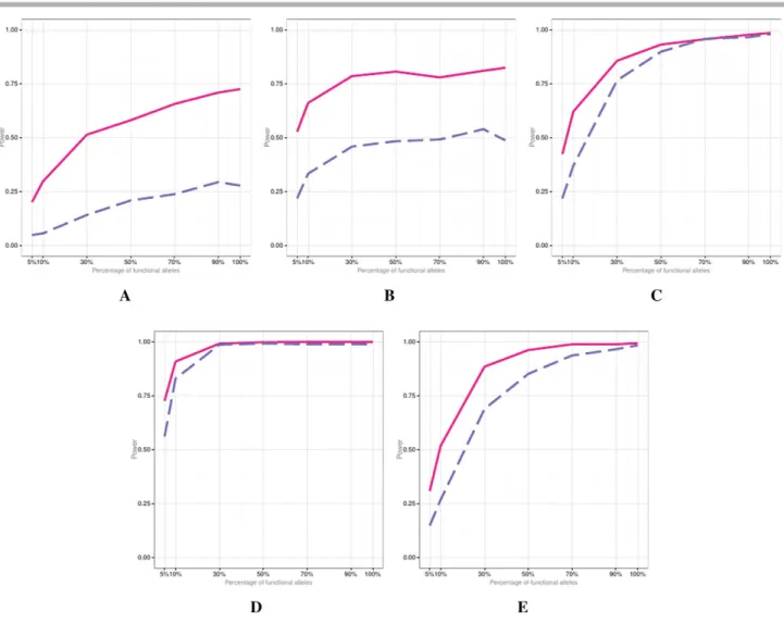
Figure 3 summarizes empirical power results for the sce-nario with risk variants having either positive or negative effects (i.e., μγ =μα=0) for the different number of sub-jects. In Figure 4 the majority of risk variants had deleteri-ous effects for both traits (i.e.,μγ>0 andμα>0). In each
216
Genetic Epidemiology, Vol. 40, No. 3, 210–221, 2016Figure 3. Empirical power of FANOVA (solid line) and SKAT (dashed line) when the variants can have either protective or deleterious effects (i.e.,μγ =μα= 0). Panel (A):N= 50, σγ =σα= 0.05; (B):N= 50, σγ =σα= 1; (C):N= 500, σγ =σα= 0.05; (D):N = 1,000, σγ =σα= 0.05; (E)
N = 2,500, σγ =σα= 0.015; (F)N= 5,000, σγ =σα= 0.015.
figure, the generalized FANOVA statistical power to detect an association between (G) and (X), while adjusting for (Z), is represented by a solid line, and the power of SKAT is repre-sented by a dashed line.
In general, the proposed FANOVA approach attained higher power than SKAT, especially for small sample sizes, small effect sizes, and when the percentage of risk variants is small. The empirical power of the two approaches become comparable if the effect sizes and the proportion of risk vari-ants were large.
Application to Real Data:
ANGPRL4
Association
with TG
To further illustrate the utility of our generalized FANOVA approach, we turn to the issue of association testing be-tween sequence variations in ANGPTL4 gene and lipid metabolism. In mice, the involvement ofANGPTL4in lipid metabolism was shown by intravenous injection of
recom-binant ANGPTL4, resulting in an increase in plasma TGs levels [Yoshida et al., 2002]. In humans, the involvement of
ANGPTL4in lipid metabolism is probable and may be asso-ciated with a higher risk of cardiovascular disorder [Kathire-san et al., 2009; Muendlein et al., 2014; Romeo et al., 2007]. However, each individualANGPTL4variant confers a mod-est effect [Kathiresan et al., 2009], suggmod-esting an improved statistical power for methods such as generalized FANOVA that perform a joint gene-based association analysis.
We conducted an analysis of 93 sequence variations in
ANGPTL4that were identified among 3,551 participants in the Dallas Heart Study [Romeo et al., 2007]. To examine an increase in plasma TG levels, we binned individuals into the “low-triglyceride” group (660 individuals with plasma TG level≤25th percentile) and into the “high-triglyceride” group (679 individuals with plasma TG level≥75th percentile). The resulting sample included 443 individuals of mixed European descent, 651 African Americans, and 245 Hispanics.
As discussed elsewhere [e.g., Svishcheva et al., 2015; Vsevolozhskaya et al., 2014], statistical power of
Figure 4. Empirical power of FANOVA (solid line) and SKAT (dashed line) when the majority of variants have deleterious effect (i.e.,μγ > 0μα> 0). Panel (A):N = 50, μγ =μα= 0.05, σγ =σα= 0.25; (B):N = 50, μγ =μα= 0.05, σγ =σα= 1; (C):N= 500, μγ =μα= 0.05, σγ =σα= 0.15; (D):
N = 500, μγ =μα= 0.25, σγ =σα= 0.15; (E):N = 1,000, μγ =μα= 0.05, σγ =σα= 0.05.
functional methods may depend on the quality of genotype data smoothing. To obtain smooth genotypic functions, we first coded allelic dosage based on the minor allele counts (i.e., either 0, 1, or 2) and applied the “flipping algorithm” [Vsevolozhskaya et al., 2014] to minimize the number of 0-2 (or 2-0) patterns in every two subsequent variant positions. However, because the majority of 93 sequenced variants were rare [Romeo et al., 2007], the coding based on minor allele counts was concluded to be optimal and no recoding of allelic dosage was necessary.
To examine an effect of increase in TG levels, modified by race and adjusted for sex, we built the following model:
ˆ
Gi(tj)=β0(tj)+β1(tj)XTGi
+β2(tj)XAAi+β3(tj)XHi+β12(tj)XTGiXAAi +β13(tj)XTGi(tj)XHi
+β4(tj)XSexi+i(tj),
where β0(tj) is the smoothed baseline allelic dosage j = 1, . . . ,93;β1(tj) is the effect of TG increase on allelic dosage. The next four terms are added to examine T×T interaction or whether the effect of TG increase varies among European Americans (β1(tj)), African Americans (β1(tj)+β12(tj)), and Hispanics (β1(tj)+β13(tj)). Finally,β4(tj) is the adjustment for sex.
To determine the most parsimonious model, we first performed a test for T×T interaction, i.e., H0:β12(tj)=
β13(tj)=0 for all tj, and found statistically significant differences in TG increasing effect among individuals of dif-ferent racial descent (P-value= 0.0028). We note that the magnitude of thisP-value remained the same for different choices of kernels and as such, we proceeded to explore spe-cific subregions of theANGPTL4gene that may harbor causal variants for the different racial groups.
Each panel of Figure 5 illustrates the estimated TG-increasing effect among different racial groups and across 93 variants of theANGPTL4gene. Further, the positions of the
218
Genetic Epidemiology, Vol. 40, No. 3, 210–221, 2016Figure 5. TG-increasing effect among European Americans (left panel), African Americans (middle panel), and Hispanics (right panel) with the 95% confidence bands (shaded regions).
recently identified variants E40K and T266M [Romeo et al., 2007; Talmud et al., 2008] are added as vertical lines to each panel. The left panel of Figure 5 shows ˆβ1(t) or the estimated
effect of TG increase among European Americans. From this panel we can infer that the region around the E40K variant has the top contribution among European Americans, be-cause it is the region over which ˆβ1(t) deviates the most from
the zero line. Additionally, the direction of ˆβ1(t) around E40K
is negative, indicating that TG increase is associated with a lower dosage of E40K variant, which implies that European American E40K carriers can be expected to have lower TG levels. However, the confidence bands for ˆβ1(t) include zero
and indicate lack of statistical significance.
The right panel of Figure 5 shows ˆβ1(t)+βˆ13(t) or the
estimated effect of TG increase among Hispanics. Once again, the effect has the top magnitude around E40K region, but its direction is reversed, indicating that Hispanic E40K carriers tend to have higher TG levels. Additionally, among Hispanics, E40K region association with TG increase reached statistical significance.
The middle panel of Figure 5 shows ˆβ1(t)+βˆ12(t) or the
estimated effect of TG increase among African Americans. Unlike European Americans and Hispanics, the contribution of E40K variant does not appear to be appreciably associated with TG increase. Also, no contribution of T266M variant to either TG increase (or decrease) was found among any racial groups.
Finally, to compare our T×T interaction results to SKAT, we performed a subgroup analysis on data from European Americans, African Americans, and Hispanics. TheP-values, adjusted for sex, for the test of an association between TG lev-els and variants in theANGPTL4gene were as follows: among European AmericansPSKAT=0.0006,PFANOVA=0.0262; among
Hispanics PSKAT=0.1738, PFANOVA=0.0001; among African
AmericansPSKAT=0.2321,PFANOVA=0.9447. Accordingly, both
methods concluded an association betweenANGPTL4 vari-ants and plasma TGs levels among European Americans, no association among African Americans, and discordant
re-sults among Hispanics. The reader should not be surprised by seemingly disagreeing FANOVA conclusions for European Americans summarized via the confidence bends in Figure 5 and via theP-value for an association test. It has been noted multiple times, including by our research group [Vsevolozh-skaya et al., 2015], that a combination of multiple “marginally significant” outcomes across different variants may result in the overall significance for a genetic region.
Discussion
By generalizing previously proposed FANOVA method-ology, we offer a novel approach not previously explored in FLM-based association studies for estimating multiple phenotype-specific effects smoothly varying over genetic variants. Furthermore, by treating genetic information as the response variable and all traits as predictors (qualita-tive or quantita(qualita-tive), the generalized FANOVA provides a straightforward way to account for hidden population strati-fication, confounders, mediators, and T×T interactions. The established connection between penalized least squares and BLUPs allows for a straightforward implementation of the proposed methodology using standard mixed linear model software.
The introduced notion of T×T interaction deserves addi-tional clarification. We are not necessarily putting emphasis on the interaction itself or the value of its coefficient. Rather, the inclusion of this term gives a simple way of detecting possible effects of various combinations of treatment and trait values that may go beyond what is captured by the sum of their individual effects.
How well do our generalized FANOVA regression coef-ficient estimates replicate what others have found in prior studies of ANGPTL4? Studies of Romeo et al. [2007] and Talmud et al. [2008] revealed that among European Amer-icans E40K carriers have significantly lower TG levels. Tal-mud et al. [2008] also showed TG-lowering effect of T266M
variant, but only among E40K carriers (i.e., whenever E40K men were excluded from the reanalysis, there was no longer a significant association between T266M and TG levels). T266M is more prevalent than E40K and in our sample out of 620 T266M carriers only 16 were also carriers of E40K, which may be a reason behind lack of association. Furthermore, no studies presented conclusive findings over TG-lowering effect and mutations inANGPTL4, so a replication of the reported association is required.
Our generalized FANOVA model is a functional model analogue of “reverse regression” [e.g., Maddala, 1992], where genetic information,X, becomes the response while pheno-types,Y, are treated as predictors. Regression coefficients are not invariant to swapping of predictor and response vari-ables. However, partial correlations, as well as test statistics and the correspondingP-values remain the same after swap-ping. Thus, effects of adjustments for covariates in a direct model are properly preserved when testing for association in a reverse model. With multiple correlated predictors at an ar-bitrary variant’s positiontj, the test statistic for the regression coefficientβican be re-expressed based on the partial corre-lation betweenYandXi, which is not affected by swapping of variables, and the test statistic (and therefore theP-value) is also invariant under the reversal in a functional model. One limitation of this approach is that for the direct and reverse tests to be equivalent,Xicannot enter any interaction terms with other variables.
The generalized FANOVA is an extension of the previ-ously proposed FANOVA approach and thus inherits some of its features. For example, generalized FANOVA fully utilizes variants’ position information and linkage-disequilibrium structure when computing the test statisticF. However, un-like the previously proposed FANOVA, our current approach allows inclusion of multiple traits and adjustment for ad-ditional covariates. Moreover, our new functional approach provides a unique way of graphically depicting phenotypic effects and interactions by representing them as continuous curves varying over a genetic region. We also hypothesize that the functional approach may hold increased robustness to genotyping errors. This may be due to the fact that the estimated genotype functions, ˆG(t), are used for the analysis in place of allele frequencies of the marked locus. It is noted that genotyping errors can have severe consequences for the analysis of low frequency alleles [e.g., Abecasis et al., 2001]. Although genotype functions are estimated via allele counts, they incorporate a certain degree of smoothing, therefore the fitted functions are expected to be less prone to genotyping errors.
In terms of the application of the generalized FANOVA methodology, practitioners can use standard mixed-effects software to estimate continuous regression coefficients as il-lustrated in Methods section of this article. Previous research in penalized regression models [Scheipl and Greven, 2012] suggests that a penalty with a small null space should be pre-ferred (a typical choice for the number of “fixed effects” is 2) and a “rule of thumb” for the number of “random effects” is
κ=35. However, the specific number of kernel functions is
unimportant as long as the fitted genotype functions are not too smooth.
Acknowledgments
This work was supported by a National Institute of Drug Abuse T32 research training program award (NIDA; T32DA021129) for OAV’s post-doctoral fellowship, DVZ’s Intramural Research Program of the National Institute of Environmental Health Sciences (NIEHS), DAB’s research award (NIDA; R01DA016558), and QL’s Mentored Research Scientist Development Award (NIDA; K01DA033346). We have no conflicts of interest to declare.
References
Abecasis GR, Cherny SS, Cardon LR. 2001. The impact of genotyping error on family-based analysis of quantitative traits.Eur J Hum Genet9(2):130–134.
Aronszajn N. 1950. Theory of reproducing kernels.Trans Amer Math Soc68(3): 337– 404.
Bouchard TJ, Jr., Loehlin JC. 2001. Genes, evolution, and personality.Behav Genet
31(3):243–273.
Brumback BA, Ruppert D, Wand MP. 1999. Comment.J Am Stat Assoc94(447):794– 797.
Carvajal-Carmona LG. 2010. Challenges in the identification and use of rare disease-associated predisposition variants.Curr Opin Genet Dev20(3):277–281. Crainiceanu C, Ruppert D, Wand MP. 2005. Bayesian analysis for penalized spline
regression using winbugs.J Stat Soft14(14):1–24.
Crainiceanu CM, Goldsmith AJ. 2010. Bayesian functional data analysis using winbugs.
J Stat Softw32(11):1–33.
De Wit H. 2009. Impulsivity as a determinant and consequence of drug use: a review of underlying processes.Addict Biol14(1):22–31.
Durbin RM, Altshuler DL, Durbin RM, Abecasis GAR., Bentley DR, Chakravarti A, Clark AG, Collins FS, and others. 2010. A map of human genome variation from population-scale sequencing.Nature467(7319):1061–1073.
Eilers PH, Marx BD. 1996. Flexible smoothing with b-splines and penalties.Stat Sci
11(2): 89–102.
Fan R, Wang Y, Mills JL, Wilson AF, Bailey-Wilson JE, Xiong M. 2013. Functional linear models for association analysis of quantitative traits.Genet Epidemiol37(7):726– 742.
Fan R, Wang Y, Mills JL, Carter TC, Lobach I, Wilson AF, Bailey-Wilson JE, Weeks DE, Xiong M. 2014. Generalized functional linear models for gene-based case-control association studies.Genet Epidemiol38(7):622–637.
Fasshauer GE. 2012. Greens functions: taking another look at kernel approximation, radial basis functions, and splines. In: Neamtu M, Schumaker L, editors. Approxi-mation Theory XIII: San Antonio 2010. New York: Springer, pp. 37–63. Fasshauer GE, Ye Q. 2013. Reproducing kernels of Sobolev spaces via a green kernel
approach with differential operators and boundary operators.Adv Comput Math
38(4):891–921.
Feng Z. 2014. A generalized quasi-likelihood scoring approach for simultaneously testing the genetic association of multiple traits.Journal of the Royal Statistical Society: Series C (Applied Statistics)63(3):483–498.
Goldsmith J, Bobb J, Crainiceanu CM, Caffo B, Reich D. 2010. Penalized functional regression.J Comput Graph Stat20(4):830–851.
Green PJ, Silverman BW. 1993.Nonparametric Regression and Generalized Linear Mod-els: A Roughness Penalty Approach. London; New York: CRC Press.
Hastie T, Tibshirani R, Friedman J, Hastie T, Friedman J, Tibshirani R. 2009.The Elements of Statistical Learning. New York, NY: Springer.
Ivanescu AE, Staicu A-M., Scheipl F, Greven S. 2015. Penalized function-on-function regression.Comput Stat30(2): 1–30.
Kathiresan S, Willer CJ, Peloso GM, Demissie S, Musunuru K, Schadt EE, Kaplan L, Bennett D, Li Y, Tanaka T, and others. 2009. Common variants at 30 loci contribute to polygenic dyslipidemia.Nat Genet41(1):56–65.
Kimeldorf G, Wahba G. 1971. Some results on Tchebycheffian spline functions.J Math Anal Appl33(1):82–95.
Kwan JS, Kung AW, Sham PC. 2011. A simple bias correction in linear regression for quantitative trait association under two-tail extreme selection.Behav Genet
41(5):776–779.
Lee D-Y, Hanis C, Bell G, Aguilar D, Redline S, Below J, Xiong M. 2014. Genetic studies of physiological traits with their application to sleep apnea.arXiv preprint arXiv:1410.7363.
Lian H. 2007. Nonlinear functional models for functional responses in reproducing kernel Hilbert spaces.Can J Stat35(4):597–606.
Liu DJ, Leal SM. 2010. A novel adaptive method for the analysis of next-generation sequencing data to detect complex trait associations with rare variants due to gene main effects and interactions.PLoS Genet6(10):e1001156.
Luo L, Boerwinkle E, Xiong M. 2011. Association studies for next-generation sequenc-ing.Genome Res21(7):1099–1108.
Luo L, Zhu Y, Xiong M. 2012a. Quantitative trait locus analysis for next-generation sequencing with the functional linear models.J Med Genet49(8):513– 524.
Luo L, Zhu Y, Xiong M. 2012b. Smoothed functional principal component analysis for testing association of the entire allelic spectrum of genetic variation.Eur J Hum Genet21(2):217–224.
MacKinnon DP, Krull JL, Lockwood CM. 2000. Equivalence of the mediation, con-founding and suppression effect.Prev Sci1(4):173–181.
Maddala GS. 1992.Introduction to Econometrics, Volume 2. New York: Macmillan. Muendlein A, Saely CH, Leiherer A, Fraunberger P, Kinz E, Rein P, Vonbank A,
Zano-lin D, MaZano-lin C, Drexel H. 2014. Angiopoietin-like protein 4 significantly pre-dicts future cardiovascular events in coronary patients.Atherosclerosis237(2):632– 638.
Nosedal-Sanchez A, Storlie CB, Lee TC, Christensen R. 2012. Reproducing kernel Hilbert spaces for penalized regression: a tutorial.Am Stat66(1):50–60. Pearce ND, Wand MP. 2006. Penalized splines and reproducing kernel methods.Am
Stat60(3):233–240.
Poggio T, Girosi F. 1990. Networks for approximation and learning. Proc IEEE
78(9):1481–1497.
Ramsay J, Silverman B. 2005.Functional Data Analysis, 2nd Edition. New York: Springer-Verlag.
Rasmussen CE, Williams CKI. 2006.Gaussian Processes for Machine Learning. Cam-bridge, Mass: Citeseer.
Reimherr M, Nicolae D. 2014. A functional data analysis approach for genetic associa-tion studies.Ann Appl Stat8(1):406–429.
Romeo S, Pennacchio LA, Fu Y, Boerwinkle E, Tybjaerg-Hansen A, Hobbs HH, Cohen JC. 2007. Population-based resequencing of ANGPTL4 uncovers variations that reduce triglycerides and increase HDL.Nat Genet39(4):513–516.
Ruppert D. 2002. Selecting the number of knots for penalized splines.J Comput Graph Stat11(4):737–757.
Ruppert D, Wand MP, Carroll RJ. 2003.Semiparametric Regression. Cambridge Uni-versity Press.
Saitoh S. 1988.Theory of Reproducing Kernels and Its Applications. Springer US: Long-man Scientific & Technical Harlow.
Scheipl F, Greven S. 2012. Identifiability in penalized function-on-function regression models. Technical Report 125, Department of Statistics, Munich: University of Munich.
Shen Q, Faraway J. 2004. An F test for linear models with functional responses.Stat Sin
14(4):1239–1258.
Smola AJ, Sch¨olkopf B. 1998.Learning with Kernels. MIT Press: Citeseer.
Speed T. 1991. [that BLUP is a good thing: the estimation of random effects]: Comment.
Stat Sci6(1): 42–44.
Storey JD, Xiao W, Leek JT, Tompkins RG, Davis RW. 2005. Significance analysis of time course microarray experiments.Proc Natl Acad Sci USA102(36):12837– 12842.
Svishcheva GR, Belonogova NM, Axenovich TI. 2015. Region-based association test for familial data under functional linear models.PLoS One10(6):e0128999. Talmud PJ, Smart M, Presswood E, Cooper JA, Nicaud V, Drenos F, Palmen J, Marmot
MG, Boekholdt SM, Wareham NJ, and others. 2008. Angptl4 e40k and t266m effects on plasma triglyceride and HDL levels, postprandial responses, and CHD risk.Arterioscler Thromb Vasc Biol28(12):2319–2325.
Vsevolozhskaya OA, Zaykin DV, Greenwood MC, Wei C, Lu Q. 2014. Functional analysis of variance for association studies.PLoS One9(9):e105074.
Vsevolozhskaya OA, Greenwood MC, Powell SL, Zaykin DV. 2015. Resampling-based multiple comparison procedure with application to point-wise testing with func-tional data.Environ Ecol Stat22(1):45–59.
Wahba G. 1990.Spline Models for Observational Data. Society for Industrial and Applied Mathematics: SIAM.
Wand M, Ormerod J. 2008. On semiparametric regression with O’sullivan penalized splines.Aust NZ J Stat50(2):179–198.
Wang Y. 1998. Smoothing spline models with correlated random errors.J Am Stat Assoc
93(441):341–348.
Wang Y, Liu A, Mills JL, Boehnke M, Wilson AF, Bailey-Wilson JE, Xiong M, Wu CO, Fan R. 2015. Pleiotropy analysis of quantitative traits at gene level by multivariate functional linear models.Genet Epidemiol39(4):259–275.
Wood S. 2006.Generalized Additive Models: An Introduction with R. Boca Raton, Lon-don, New York: Chapman & Hall/CRC Texts in Statistical Science.
Wu CO, Yu KF. 2002. Nonparametric varying-coefficient models for the analysis of longitudinal data.Int Stat Rev70(3):373–393.
Wu MC, Lee S, Cai T, Li Y, Boehnke M, Lin X. 2011. Rare-variant association testing for sequencing data with the sequence kernel association test.Am J Hum Genet
89(1):82–93.
Yoshida K, Shimizugawa T, Ono M, Furukawa H. 2002. Angiopoietin-like protein 4 is a potent hyperlipidemia-inducing factor in mice and inhibitor of lipoprotein lipase.
J Lipid Res43(11):1770–1772.
Zhang J-T. 2013.Analysis of Variance for Functional Data. Boca Raton, London, New York: CRC Press.
Zhu Y, Xiong M. 2012. Family-based association studies for next-generation sequenc-ing.Am J Hum Genet90(6):1028–1045.