Advances in Reliability, Risk and Safety
Analysis with Big Data: Proceedings of
the 57th ESReDA Seminar
Hosted by the Technical
University of Valencia,
23-24 October, 2019,
Valencia, Spain
Ferreira, L. A., Simola, K., Kopustinskas, V
This publication is a Conference and Workshop report by the Joint Research Centre (JRC), the European Commission’s science and knowledge service. It aims to provide evidence-based scientific support to the European policymaking process. The scientific output expressed does not imply a policy position of the European Commission. Neither the European Commission nor any person acting on behalf of the Commission is responsible for the use that might be made of this publication. For information on the methodology and quality underlying the data used in this publication for which the source is neither Eurostat nor other Commission services, users should contact the referenced source. The designations employed and the presentation of material on the maps do not imply the expression of any opinion whatsoever on the part of the European Union concerning the legal status of any country, territory, city or area or of its authorities, or concerning the delimitation of its frontiers or boundaries.
EU Science Hub https://ec.europa.eu/jrc JRC122223
EUR 30415 EN
PDF ISBN 978-92-76-23807-2 ISSN 1831-9424 doi:10.2760/836400
Luxembourg: Publications Office of the European Union, 2020.
© European Union, 2020
The reuse policy of the European Commission is implemented by the Commission Decision 2011/833/EU of 12 December 2011 on the reuse of Commission documents (OJ L 330, 14.12.2011, p. 39). Except otherwise noted, the reuse of this document is authorised under the Creative Commons Attribution 4.0 International (CC BY 4.0) licence (https://creativecommons.org/licenses/by/4.0/). This means that reuse is allowed provided appropriate credit is given and any changes are indicated. For any use or reproduction of photos or other material that is not owned by the EU, permission must be sought directly from the copyright holders.
All content © European Union, 2020.
How to cite this report: Ferreira, L.A., Simola, K. and Kopustinskas, V., Advances in Reliability, Risk and Safety Analysis with Big Data: Proceedings of the 57th ESReDA Seminar, EUR 30415 EN, Publications Office of the European Union, Luxembourg, 2020, ISBN 978-92-76-23807-2, doi:10.2760/836400, JRC122223.
European Safety, Reliability & Data Association (ESReDA) is a European Association established in 1992 to promote research, application and training in Reliability, Availability, Maintainability and Safety (RAMS). The Association provides a forum for the exchange of information, data and current research in Safety and Reliability.
The contents of ESReDA seminar proceedings do not necessarily reflect the position of ESReDA. They are the sole responsibility of the authors concerned. ESReDA seminar’s proceedings are designed for free public distribution. Reproduction is authorized provided the source is acknowledged.
ESReDA membership is open to organisations, privates or governmental institutes, industry researchers and consultants, who are active in the field of Safety and Reliability. Membership fees are currently 1000 EURO for organisations and 500 EURO for universities and individual members. Special sponsoring or associate membership is also available.
For more information and available ESReDA proceedings please consult: http://www.esreda.org/
Table of contents
Preface………..…..…………1 System health monitoring with deep learning: Is big data all we need?...2 Recommended practice for assurance of data-driven algorithms and models ………..…4 Fleet-based remaining useful life prediction of safety-critical electronic devices ……...…...12 Assessing GB train accident risk using red aspect approaches to signal data………...……...20 Quality in big data for the forced unavailability of power plants……….………..……..33 Mechanical seal failure prediction in an oil refinery: a first attempt to solve the problem using a data-driven approach (abstract) ...……….………...66 Trust in AI: The role of hybrid and private governance ..………..…...…...68 Advanced analysis of reliability and risk of equipment subjected to degradation and
obsolescence………...……….……….88 Robust statics for (big) Data Analytics (abstract)….………...………..….……...……...96 A proposal of an algorithm to simulation right censored data type I in reliability field
(abstract)……….………...……...99 IOT future in energy industries (abstract)………...…….…..…100 List of authors……….101
Appendix 1: Slide presentations Appendix 2: Seminar Programme
Preface
The 57th Seminar organized by ESReDA took place in the very beautiful city of Valencia, Spain. We were very kindly received by the Polytechnic University of Valencia/Universitat Politècnica de Valencia.
The Seminar was jointly organized by ESReDA and CMT Motores Termicos, a research unit at the Polytechnic University of Valencia. A sincere thanks is due to Professor Bernardo Tormos for the way he received us and allowed the Seminar to precede according to our best expectations.
In accordance with the theme proposed for the Seminar, communications were presented that made it possible to discuss and better understand the role of the latest big data, machine learning and artificial intelligence technologies in the development of reliability, risk and safety analyses for industrial systems.
The world is moving fast towards wide applications of big data techniques and artificial intelligence is considered to be the future of our societies. Rapid development of 5G telecommunications infrastructure would only speed up deployment of big data analytic tools. However, despite the recent advances in the these fields, there is still a long way to go for integrated applications of big data, machine learning and artificial intelligence tools in business practice.
We would like to express our gratitude to the authors and key note speakers in particular and to all those who shared with us these moments of discussion on subjects of great importance and topicality for the members of ESReDA.
The editorial work for this volume was supported by the Joint Research Centre of the European Commission in the frame of JRC support to ESReDA activities. A special thanks is due to Ariane Liessens (JRC) for the editorial work.
Dr. Vytis Kopustinskas, Dr. Kaisa Simola Prof. Luís Andrade Ferreira
System health monitoring with deep learning:
Is big data all we need?
Olga Fink ETH Zürich
Abstract
Deep learning and artificial intelligence have achieved some impressive successes in many different domains. These technologies applied in computer vision, natural language processing and speech recognition are gradually becoming an integral part of people’s everyday lives. Concurrently, increasing amounts of condition monitoring data have been captured by complex industrial assets in many different industries, including energy and transportation. But what is the potential of these emerging technologies and “big data” for system health monitoring? Where could the development go and how could potential transformation look like? How could deep learning and artificial intelligence be integrated in decision making of asset managers supporting them to make optimal decisions?
While large amounts are captured on the condition of complex systems, faults in safety critical systems are rare. The diversity of the fault types and operating conditions makes it often impossible to extract and learn the fault patterns of all the possible fault types affecting a system. Consequently, faulty conditions cannot be used to learn patterns from. Supervised learning that has made most of the current success of AI possible is, therefore, often not applicable in the context of system health monitoring.
Even collecting a representative dataset with all possible operating conditions can be a challenging task since the operating conditions of complex industrial systems are highly varying. Therefore, training samples captured over short time periods may not be representative for the entire operating profile. Collecting datasets over longer time periods could capture more operating profiles and, thereby, improve the representativeness. However, that would also delay the point in time when the data-driven health monitoring systems could be taken into operation. Such delays are often not acceptable in real applications. We need, therefore, to rely on datasets that are not fully representative and have either none or very few faults and integrate the missing information either from other units of a fleet or from physical performance models.
The talk will give some insights into current challenges and highlight potential solutions for fault detection, isolation and the prediction of the remaining useful lifetime in the context of rare faults and a high variability of operating conditions. The talk will particularly present solutions in the field of domain adaption, transferring models between different units of a fleet and between
different operating conditions, and hybrid approaches fusing physical performance models and deep neural networks.
References:
Fink, Olga, Qin Wang, Markus Svensén, Pierre Dersin, Wan Jui Lee, and Melanie Ducoffe. 2020. “Potential, Challenges and Future Directions for Deep Learning in Prognostics and Health Management Applications.” Engineering Applications of Artificial Intelligence 92 (June): 103678. https://doi.org/10.1016/j.engappai.2020.103678.
Recommended Practice for Assurance of Data-driven
algorithms and models
Siegfried Eisinger, Jon Arne Glomsrud & Justin Fackrell DNV GL. Norway
1. Introduction
Systems incorporating Machine Learning, and other data-driven techniques, have become increasingly widespread in recent years. Large organizations, such as Google, Alibaba and Amazon have capitalized on the capabilities of such techniques to do things better, do things faster, and/or do things previously impossible.
In industrial contexts too, data-driven techniques are being used in a variety of applications including:
• Early detection of failures (before they happen) and Condition-Based Maintenance (CBM)
• Semi- and fully-automated technical verification
• Simplifications and effectiveness improvements in class services (currently carried out manually by surveyors)
The goal of many data-driven applications is to facilitate decision support for an end user. End users are often people and/or organizations, but they can also be autonomous agents. The data from which data-driven models are derived is often very large and complex, and the models themselves are also complex. This complexity leads to challenges in establishing trust on the part of the user that a given data-driven system will perform as required. In a Recommended Practice (RP), DNV GL addresses these challenges by defining a framework for establishing trust in data driven models. The RP is currently in a draft stage and will be published end of 2019.
The goal of the RP is to help readers answer the following question: How can the user of an application which is based on a data-driven model be sure that the model is suitable for the intended use, and that the risk of failure and/or bad output is kept within tolerable limits?
To date no widely-recognized standard exists for assessment of a data-driven model. The current RP provides a structured approach for performing such an assessment. It makes use of CRISP-DM (The Cross-Industry Standard Process for Data Mining), a de-facto standard process for data-driven modelling. CRISP-DM was developed by an industry consortium in the ESPRIT European project.
Note that throughout the paper, we often use the word ‘algorithms’ as an abbreviation for ‘data- driven algorithms and models’.
2. Approach
Assurance of algorithms concerns the verification and validation that the algorithm is suitable for its intended use and in a wider context it also includes whether the intended use is according to rules, regulations and societal agreements. It should thus be possible to check any outcome of the algorithm with respect to whether it is acceptable or not. Moreover, it should be possible to predict all relevant algorithm outcomes, so that they can be checked. Obviously, full prediction and check of all possible outcomes is only possible for the simplest algorithms and for any real-world algorithm we are left with checking sub-sets. As algorithm complexity increases it gets more and more difficult to claim any sort of test completeness. Therefore, to base an assurance regime on the test of a finished algorithm becomes questionable. Even if it was possible to ensure a good test coverage, decisions during earlier stages in the lifecycle might have been flawed, leading to errors in the test specification and thus to faults which cannot be uncovered by the test. This leads to the statement
Assurance of complex systems cannot be based on verification and validation testing alone Effective verification can only be performed if the scope is sufficiently limited. In addition, the stages of the lifecycle must be taken into account, ensuring that the output of one stage does not invalidate the results from previous phases, but supports the general goal. For example, even a perfect system which is put into operation might become flawed when maintenance is not performed in a correct way. Or, even a perfect design process will lead to a flawed product if the initial specification is flawed. This is the reason why many standards for assurance of complex systems adopt the strategy
Quality Assurance of complex systems should be done through quality assurance of all relevant lifecycle stages
This strategy has been implemented in for example IEC 61508 /1/ and other similar standards for reliability of critical systems.
One might object that some systems can be checked with 100% coverage through so-called Formal Proofs: Given that the basic specification is correct it can be checked that the system behaves completely according to that specification. It is true that such systems in principle can be approved through only testing, but systems which have a complete formal proof are seldom. Beyond that, performing a bad quality development process would most probably reveal a lot of errors through the formal proof, rendering the development process inefficient because of the error correction efforts they require. It would therefore most probably be most efficient to perform the suggested QA steps throughout the lifecycle and arrive at a work product with few errors, confirmed through formal proof.
Lifecycle schemes are often linked to Risk Analysis. Through the initial risk analysis the integrity requirements of the system are determined. Low integrity requirements would lead to less stringency with respect to QA rules than high integrity requirements. This approach has merits, rendering the life-cycle process into a ‘risk-based’ quality approach, focusing on critical issues and systems, while less critical issues and systems are treated in a more basic way. In IEC 61508 the first risk analysis is placed at the start of the lifecycle
process after the concept is specified and it is used to perform the so-called Safety Integrity Level (SIL) allocation. The SIL is a four-level system linking the safety functions to the expected reliability with which it shall be delivered. The SIL is in turn linked to QA requirements throughout the lifecycle, their rigor increasing with increasing SIL. Table 1 quotes Table A.5 of /1/ for Software module testing and integration as one example, clearly demonstrating the basic requirement and the rigor increasing with the SIL.
Table 1 Copy of Table 4.5 of /1/. Software module testing and integration. R: ‘Recommended’, HR: ‘Highly Recommended’
Technique/Measure SIL 1 SIL 2 SIL3 SIL 4
1 Probabilistic testing - R R R
2 Dynamic analysis and testing R HR HR HR
3 Data recording and analysis HR HR HR HR
4 Functional and black box testing HR HR HR HR
5 Performance testing R R HR HR
6 Model based testing R R HR HR
7 Interface testing R R HR HR
8 Test management and automation tools R HR HR HR 9 Forward traceability between the software design
specification and the module and integration test specification
R R HR HR
10 Formal verification - - R R
Accepting the two above statements, that assurance cannot be based on testing alone and that quality must be taken into account throughout the lifecycle our suggestion for an assurance regime for data-driven algorithms and models is based on a strategy similar to IEC 61508. The lifecycle model for data-driven algorithms and modules’ is not identical to general software development, where often the V-model or a variant thereof is employed. For data mining projects the Cross-industry Standard Process for Data Mining (CRISP-DM) has been defined by an industry consortium in the ESPRIT European project (see /2/). This process has been accepted as a de-facto standard in the area, leading to the decision that it is also used in the present RP as basis.
3. The RP
Our framework for assurance of Data-driven Algorithms and models is due to be presented in full detail in the Recommended Practice DNVGL-RP-0510/3/, but the key concepts are presented here. The framework is structured around the CRISP-DM reference model/2/, as motivated in the previous section. The lifecycle model is structured along
both a linear development process and explicit feedback stages both on a local level (e.g. between ‘data preparation’ and ‘modelling’) and on a more global level (e.g. between ‘business understanding’ and ‘evaluation’). Compared to the software development V-model, the CRISP-DM model includes more relations to the proper understanding of the basics and explicit evaluation stages. The main reason for that might be that CRISP-DM was originally designed for business supporting tools, as opposed to critical applications. On the other hand, also for critical applications it is important to establish a correct ‘problem understanding’ and ‘data understanding’. Before deployment a proper verification and validation phase must be included (i.e. ‘evaluation’), demonstrating that the basic lifecycle steps seem to work for a wide area of applications.
The CRISP-DM process can be used in any assurance project regardless of the explicit usage of CRISP- DM during product development. The CRISP-DM workflow was developed in the late 1990’s and has gained wide acceptance and popularity in the field of data science and machine learning, which was the main reason why we have decided to re-use the related lifecycle process.
Figure 1 Phases of the CRISP-DM reference model (ref. /2/, Figure 2)
Trust in an algorithm is established through the construction of an assurance case: this is a structured document containing detailed claims. Associated with each claim is one or more items of evidence which together support that claim. For example, in the activity data preparation, the claim “the data
is representative” may be supported by evidence showing that “the data is drawn from a group of 15 assets over 5 years, plus analysis confirming that this sample satisfactorily covers the feature space”.
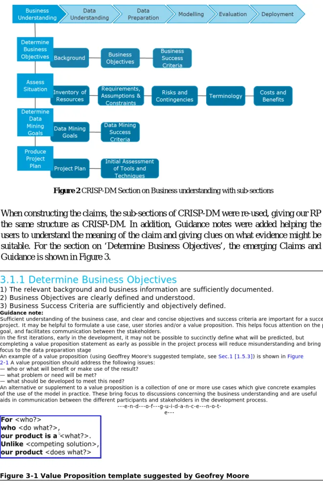
CRISP-DM offers more than the reference model of Figure 1. Each of the lifecycle stages is supported by sub-sections in two levels. In Figure 2 the sub-sections of Business Understanding are shown.
3.1.1 Determine Business Objectives
1) The relevant background and business information are sufficiently documented. 2) Business Objectives are clearly defined and understood.
3) Business Success Criteria are sufficiently and objectively defined.
Guidance note:
Sufficient understanding of the business case, and clear and concise objectives and success criteria are important for a successful project. It may be helpful to formulate a use case, user stories and/or a value proposition. This helps focus attention on the project goal, and facilitates communication between the stakeholders.
In the first iterations, early in the development, it may not be possible to succinctly define what will be predicted, but completing a value proposition statement as early as possible in the project process will reduce misunderstanding and bring focus to the data preparation stage
An example of a value proposition (using Geoffrey Moore's suggested template, see Sec.1 [1.5.3]) is shown in Figure 2-1 A value proposition should address the following issues:
—who or what will benefit or make use of the result? —what problem or need will be met?
—what should be developed to meet this need?
An alternative or supplement to a value proposition is a collection of one or more use cases which give concrete examples of the use of the model in practice. These bring focus to discussions concerning the business understanding and are useful aids in communication between the different participants and stakeholders in the development process.
---e-n-d---o-f---g-u-i-d-a-n-c-e---n-o-t-e---
Figure 3-1 Value Proposition template suggested by Geofrey Moore Figure 2 CRISP-DM Section on Business understanding with sub-sections
When constructing the claims, the sub-sections of CRISP-DM were re-used, giving our RP the same structure as CRISP-DM. In addition, Guidance notes were added helping the users to understand the meaning of the claim and giving clues on what evidence might be suitable. For the section on ‘Determine Business Objectives’, the emerging Claims and Guidance is shown in Figure 3.
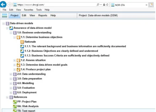
The evidence must obviously be provided on a per -project basis. To facilitate this process, the content of the RP has been translated into the Argumentation tool REASON/4/. This tool can be used in an interactive fashion between all stakeholders. The provider of the algorithm can perform an initial self-assessment, entering all evidence which seems relevant. An independent assessor can then check the provided evidence and enter scores on whether the evidence is sufficient, or what other evidence is needed. Relevant parts of the assessment can be re-run when anything in the algorithm, the basic data or the usage area changes. Figure 4 shows an extract of the RP as it is implemented in REASON.
Figure 4 The RP implemented into the argumentation tool REASON
The stringency of the requirements on the evidence depends on the criticality and the uncertainty the application represents: higher consequence applications have a higher level of rigour, and thus more strict requirements on evidence. For example, an ML algorithm whose job is to suggest classifications of documents to a human user has a low criticality (there is no substantial risk to safety or asset integrity if a suggestion is wrong, since the human user can ignore the suggestion) but an ML algorithm which pre-sorts asset condition data into “OK”/“needs attention” where the human operator only looks at the “needs attention” cases has higher criticality and so has more extensive requirements on evidence. Similarly, if techniques are employed where there is little experience, or where the results are hard to check, the uncertainty increases, giving rise to a higher risk rating and thus more stringent evidence requirements. In a future version of the RP this might be elaborated into requirements tables like Table 1, but more research and development is needed for that.
4. Case Studies
Parallel with the development of the RP, a number of Use Cases have been run. The cases concern practical applications like mooring prediction, wear detection and remaining useful life estimation. The anonymized findings from the use cases are shown in Table 2. The findings demonstrate that Assurance of digital assets is needed and that the areas which are in focus in the upcoming Recommended Practice are relevant.
Table 2 Findings from the Use Cases run during the development of the Recommended Practice
Finding Possible consequences Use cases
affected No baseline model • Model overengineered (a much simpler
model would do) A, B, D
No quantitative evaluation • Unknown performance, impossible to use as
basis of business decisions A, E Model only tested on
simulation data not real data • Jump to real world may include surprises A, D Model’s computational
feasibility is in question • Cannot be used in practice B Not enough training cases • Model is undertrained B Model does not generalize • Model won’t be able to deal with
situations it hasn’t seen before, i.e. it doesn’t really learn anything
B
Intended use not properly
understood • Surprises at deployment time C
Criticality not established • Can’t make business decision based on
quantitative performance C, D, B, A Data available is out of date • Even if project succeeds, not clear path to a
future deployment C
Quality of human-labelled
data unknown • Uncertainty in performance, and “howgood is perfect?” C Evaluation metric is
misleading • “You fool yourself, and you are the easiestperson to fool” D
No held-out evaluation data • Overfitting E
Training data not
representative • Surprises at deployment time E
Retraining plan is adhoc • No systemetic quality E No continuous monitoring of
performance • Performance can degrade E
Susceptibility to security
5. Future Work
With respect to the future of this RP the following is foreseen
• Perform the formal review process for the RP (also including external reviews) prior to finalizing the RP and then publishing within the framework of rules.dnvgl.com
• Use results from the current research programme ‘Assurance of Digital Assets’ (ADA) to improve the RP with more recommendations on methods and techniques which should be used – in dependence on risk if relevant.
• So far, the assurance regime is process-centric, as motivated in Section 2. It does still make sense to add recommendations on how the model/algorithm itself should be validated. A Recommended Practice on Data Quality already exists (see /6/) and the two RPs are closely linked.
• CRISP-DM has been criticised for not including enough on the operational side, as data-driven models are not necessarily stable in this respect and need review and modification to stay useable. The RP should be improved in this respect.
References
[1] IEC 61508. Functional safety of electrical/electronic/programmable electronic safety-related Systems. IEC. Ed. 2. 2010
[2] CRISP-DM 1.0. Step-by-step data mining guide. SPSS. 199
[3] DNVGL-RP-0510. Recommended Practice for the Assurance of Data-driven Algorithms and Models. DNV GL. 2019. To be published.
[4] REASON. NOR-STA support system for achieving and assessing conformance to NORms and STAndards. See www.nor-sta.eu
[5] DNVGL-RP. Set of official Recommended Practice guidelines published by DNV GL. See https://rules.dnvgl.com
[6] DNV GL, DNVGL-RP-0497 Recommended practice: Data quality assessment framework. 2017. http://rules.dnvgl.com/docs/pdf/dnvgl/rp/2017-01/dnvgl-rp-0497.pdf.
Fleet-Based Remaining Useful Life Prediction of
Safety-critical Electronic Devices
Mathias Verbeke, Alessandro Murgia, Tom Tourwé, Elena Tsiporkova Data and AI Competence Lab, Sirris Bd. A. Reyerslaan 80,
B-1030 Brussels BELGIUM
Abstract
Since ever more assets get connected to the Internet, an increasing amount of data is gathered on an asset’s operating environment and its respective usage conditions. This enables one to closely monitor the behaviour of an asset during its lifetime and extract useful insights in a data-driven way. For complex assets operating in safety- critical environments, knowledge on their remaining useful lifetime is often invaluable, for example to proactively schedule maintenance interventions and avoid unwanted downtime. When a new asset type is introduced, however, limited to no historical data on other assets of this new type that were observed towards their end of life and can be used to learn a RUL prediction model is available. Consequently, traditional techniques to perform RUL prediction often fall short in this case. In this paper, a methodology that leverages the data of the entire fleet of assets to predict the RUL of new assets is presented, allowing to generalize across the behaviour of assets in different operating conditions. The methodology was validated on an industrial dataset of a fleet of electronic devices operating in safety-critical environments. Keywords: fleet-based analytics, remaining useful life prediction, electronic devices, new asset types
1. Introduction
An important concept in reliability engineering is the asset’s remaining useful lifetime (RUL), which is defined as the time the asset is likely to operate before it requires repair or replacement. Knowledge on the RUL allows avoiding unplanned downtime, proactively scheduling maintenance and optimizing the asset’s operational efficiency. This is especially relevant for assets that are operating in safety-critical settings.
Due to the trend towards Internet-of-Things, an increasing amount of data is gathered on the asset’s operating environment and the respective usage conditions. This has given rise to an extensive body of research in predicting the RUL of industrial assets in a data-driven way, using statistical or machine learning techniques. The approach to tackle this problem typically depends on the data that is available, for example using a threshold-based approach based on a set of inferred health indicators, or by extrapolating the gathered sensor values and comparing those to run-to-failure data from in-the-lab test setups gathered during product development.
Complex assets are characterized by a high amount of parameter settings and are used in a wide variety of operating conditions. This leads to a large number of degrees of
freedom, due to which it becomes hard to determine fixed health indicator thresholds or generate run-to-failure data for each of these conditions. Furthermore, typically a range of different asset types exists. When a new asset type is introduced, limited to no historical data on other assets of this new type that were observed towards their end of life and can be used to learn a RUL prediction model is available. Consequently, techniques to perform RUL prediction often fall short in this case. In order to meet this challenge, a methodology that leverages the data of the entire fleet of assets to predict the RUL is presented, allowing to generalize across the behaviour of assets in different operating conditions. The methodology was validated on an industrial dataset of a fleet of electronic devices operating in safety-critical environments.
2. Related work
Remaining useful life prediction is one of the activities that is enabled by monitoring product usage. Usage monitoring is a fundamental element in systems that assess the on-going health of a product or system, provide advance warning of failure, and provide information to improve the design and qualification of fielded and future products [1]. It is often denoted to Prognostics and Health Management (PHM) that links studies of failure mechanisms to system lifecycle management.
Usage monitoring has mainly been employed in the context of design and reliability tests, in which electronic devices such as desktops [2], notebooks [3], refrigerators [4], and game consoles [5] have been subjected to different types of loads (thermal, physical, electrical, etc.) to test their resilience. Most of these tests are performed by in-the-lab trials or small-scale field studies with actual users. More recently, Funk et al. [5] have proposed a methodology to build automatic observation modules into products, collect usage data, and analyze these data by means of process mining techniques in order to exploit in-the-field data by actual users and involve them in the development of such products earlier on. Next to (hardware) design and reliability, this also allows to more deeply study the interaction of the user with the product. The main focus of this paper is on remaining useful lifetime prediction of (safety- critical) electronic devices, due to which the attention will be focused on related work in this subdomain. Okoh et al. [6] provide an overview of RUL techniques that are used in Through-life Engineering Services, i.e., services that aim to improve support services by providing run-to-failure information for better decision making. The authors present a classification of techniques used in RUL prediction for optimisation of products’ future use based on current products in-service with regard to predictability, availability and reliability.
An increasing amount of research is also looking into hybrid approaches to predict the RUL. For example, Cheng and Pecht [7] propose a fusion prognostics method for RUL prediction of electronic products. In their approach, the PoF method is used to identify the critical parameters, identify and prioritize the potential failure mechanisms, identify the failure models, and define the failure criteria in terms of the isolated parameters, whereas the data-driven method is used to extract the features from the monitored parameters, create a healthy baseline, and compare the monitored parameters with the baseline to conduct anomaly detection and trend the isolated
Asset
parameters. The approach is validated using a case study to predict the RUL of multilayer ceramic capacitors.
For a full overview of data-driven techniques for RUL prediction, we refer the interested reader to the recent book of Si, Zhang and Hu [8]. The book of Pecht and Kang [9] specifically focusses on prognostics and health management of electronics, including an overview of knowledge-based and data-driven techniques for remaining useful life prediction. To the best of our knowledge, however, no approaches exist to predict the remaining useful lifetime of new asset types on with limited information is available, based on the exploitation of the historic data of the fleet.
3. Case study: safety-critical electronic devices
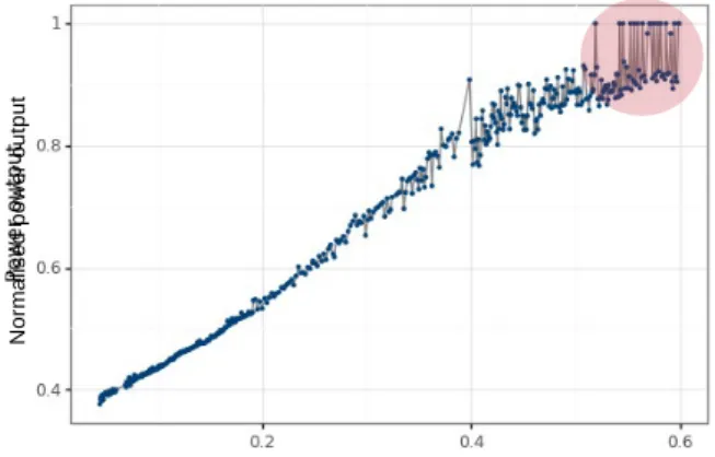
The resulting methodology was validated on a real-world industrial case study. It involves a fleet of commercially available electronic devices that are used in safety- critical environments. From this product around 50 models are available, with a total installed base of around 100k devices. For each of the assets in the fleet, the power output as well as a number of device settings such as energy intensity are available over the lifetime of the device. A number of these device settings are set by the maintenance technician during fixed calibration interventions, as well as during finetuning by the end user. For the case study, we will focus solely on the power output of the asset which increases over time until the asset fails and reaches its end of life. This is illustrated in Figure 1, showing the power output evolution of a single functional unit until it reaches its end of life (marked in red).
End of life
Figure 1: Power output evolution until the end of life of a single asset
4. Methodology
This section describes the methodology on a conceptual level. It consists of three main steps. First, assets operating in similar conditions are clustered together. Subsequently, for each of these groups, a so-called reference curve is calculated. This represents the prototypical behaviour of the assets in that particular group during their lifetime. To predict the RUL of a new asset, the top N most similar reference curves are identified and the average RUL of the assets in that cluster is determined. Finally, the RUL of the new asset is calculated as the weighted sum of these respective
Asset runtime, relative to global maximum
N o rm a lis e d pow er out put
Asset runtime
lifetimes. Each of these steps will now be discussed in more detail, taking the use case as illustrative example to demonstrate the approach.
Step 1: Clustering assets operating in similar conditions
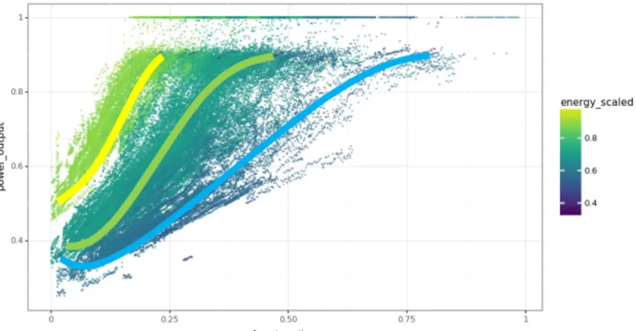
Based on an extensive exploration of the data available on the entire fleet of assets, a clear difference in behaviour can be observed. Figure 2 depicts the energy intensity of the entire fleet of assets and clearly reveals a diverse behaviour across the fleet with several energy intensity modes.
Figure 2: Energy intensity of the entire fleet of assets
To extract distinguishing behaviour across the fleet, the energy intensity curves of the entire fleet of assets are clustered using k-means clustering1 1 . This is an
unsupervised machine learning algorithm which partitions n observations into k clusters. As the name indicates, each asset is assigned to the cluster with the nearest mean, serving as a prototype of the cluster.
The most important hyperparameter of the k-means algorithm is k, denoting the number of clusters to be formed. In the proposed approach, a silhouette cluster validation analysis is used in order to determine the optimal number of clusters. It studies the separation distance between the resulting clusters. The silhouette score
ranges from −1 to +1, where a higher score indicates a better cluster separation.
For the case study, a silhouette analysis was performed in which cluster solutions with 4 up to 15 clusters were tested. The highest silhouette score was obtained using 5 clusters. The resulting clusters are depicted in Figure 3. Each of the clusters shows a different behaviour of the evolution of the energy intensity over the assets’ lifetime. The slope of the curves is the main distinguishing characteristic, representing the speed at which the assets degrade over time.
Figure 3: Clustering of the energy intensity curves with 5 clusters
Step 2: Extraction of a reference curve per cluster
In a second step, a reference curve per cluster is extracted. To calculate these reference curves, the median per timestamp across all energy intensity curves of the assets in the respective clusters are calculated.
The reference curves for the extracted clusters in the case study dataset (Figure 3) are shown in Figure 4. The region within one standard deviation (std) around the reference curves is also marked, showing that this limited boundary already captures quite some behavioural variation in the energy intensity, as these regions largely overlap with the point clouds from the clusters in Figure 3.
Figure 4: Median reference curves per energy intensity cluster
Step 3: Calculation of the RUL of the new asset
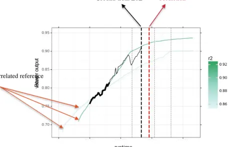
In the third and last step of the proposed approach, the remaining useful lifetime of an asset of a new type is calculated. This entails the following 4-step workflow, which will be illustrated by means of the prediction result on a prototypical asset as shown in Figure 5:
a. First, the available data on the new asset is compared to each of the reference curves. To this end, the coefficient of determination, denoted as R2 is calculated. This coefficient measures the goodness-of-fit between the available new asset data and the corresponding part of each of the reference curves. More specifically, it provides a measure of how well the new asset data points are replicated by the respective reference curve, based on the proportion of total variation of new asset data points explained by the reference curve.
black line at the start) is compared with the respective fragments of each of the reference curves. Note that the thin black line indicates the subsequent evolution of the power output until the asset reaches its end of life. This latter part is however treated as unseen data and is consequently not taken into account in the comparison with the reference curves.
b. Subsequently, the top m most similar reference curves are determined, which have an R2 correlation metric above a fixed threshold. In the example, the top 3 reference curves with an R2 score of above 50% are retained. These curves are shown in green on Figure 5, in which the color intensity indicates the degree of correlation (according to the color scale on the right).
c. In the third step, the end of lifetime of the retained top m reference curves is calculated.
d. Finally, the end of lifetime and the corresponding remaining useful life of the new asset is calculated as the weighted sum of the end of lifetime values of the retained top m reference curves as determined in the previous step. The weight factors are based on the normalized correlation strength. In the example plot, the ground truth end of lifetime is indicated with a vertical black dashed line, whereas the predicted end of lifetime is indicated with a vertical red dashed line.
Ground truth EoL Prediction
Top 3 most correlated reference curves
Figure 5: Prediction of the remaining useful lifetime of an asset of a new type
5. Validation
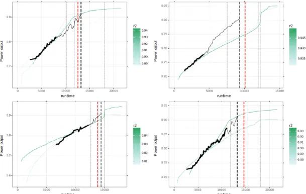
In order to validate the proposed approach, it was tested on two different subsets that differ in the amount of time within which the assets will reach their end of life. The first subset contains assets on which data is available for three quarters of their lifetime, and thus will reach their end of life in the remaining quarter. In the second subset, only data on half of the lifetime of the assets under investigation is available. The training set which was used to extract the reference curves consists of around 8.500 assets. Each of the test sets contains data of 50 new devices. For both the training and test sets, only assets of which the data was sufficiently qualitative (e.g., small percentage of missing data, no user interventions) were considered.
Po w er o ut p ut
For each of the test sets, the end of lifetime and remaining useful life of each of the assets is calculated. For both datasets, an average accuracy of around 3-5% of the average lifetime over all assets in the fleet is obtained. The results for 4 example assets from the test set are depicted in Figure 6. While the current validation results look promising, a more extensive experimental validation will be performed in future work, considering a larger amount of assets from the full range of asset lifetimes. Furthermore, also a comparison to an overall model that predicts the RUL without distinguishing between the different operating conditions of the assets in the fleet is planned.
Figure 6: RUL prediction results on four example assets from the test set
6. Conclusions and Future Work
In this paper, a methodology was proposed to predict the remaining useful lifetime of new types of safety-critical assets on which little information is known at the start of the lifetime. This is done by leveraging the available historical data on the fleet of assets of former product types, which allows one to generalize across the behaviour of assets in different operating conditions. The preliminary validation experiments show that using the proposed approach, it becomes possible to predict the RUL with a reasonable accuracy.
In future work, it will be investigated if the accuracy can be further improved by exploring alternative (machine learning-based) RUL prediction models to complement or replace the current approach based on median reference curves per cluster. Also, the current methodology only takes the energy intensity into account to characterize the behaviour of assets in the fleet. In future work, the aim is to extend this with additional variables, e.g., to better take the variation in parameter settings into account throughout the lifetime of an asset. Finally, a more extensive error
P ow er out put P ow er out put
analysis will be performed to gain deeper insight into how to improve the weighted sum when calculating the remaining useful lifetime of new assets based on the end of lifetimes of the reference curves.
Acknowledgements
A substantial part of this work was performed by dr. Paul Teehan during his time at the Data and AI Competence Lab of Sirris. This work was supported by Flanders Innovation & Entrepreneurship (VLAIO) through the SBO project HYMOP (150033) and the Federal Public Service Economy through the project BitWind.
References
[1] N. Vichare, P. Rodgers, V. Eveloy, and M. Pecht, “Environment and Usage Monitoringof Electronic Products for Health Assessment and Product Design,” Qual. Technol. Quant. Manag., vol. 4, no. 2, pp. 235–250, Jan. 2007.
[2] D. Searls, T. Dishongh, and P. Dujari, “A Strategy for enabling datadriven product decisions through a comprehensive understanding ofthe usage environment,” in Proceedings of the Pacific RIM/ASME International Intersociety Electronic and Photonic Packaging Conference (IPACK’01), Kauai, Hawaii, 2001, pp. 1279–1284.
[3] N. Vichare, P. Rodgers, V. Eveloy, and M. G. Pecht, “In Situ Temperature Measurement of a Notebook Computer—A Case Study in Health and Usage Monitoring of Electronics,” IEEE Trans. Device Mater. Reliab., vol. 4, no. 4, pp. 658–663, Dec. 2004.
[4] X. Yang, P. R. Moore, C.-B. Wong, J.-S. Pu, and S. K. Chong, “Product lifecycle information acquisition and management for consumer products,” Ind. Manag. Data Syst., vol. 107, no. 7, pp. 936–953, Aug. 2007.
[5] M. Funk, A. Rozinat, A. K. Alves de Medeiros, P. van der Putten, H.
Corporaal, and W. van der Aalst, “Improving Product Usage Monitoring and Analysis with Semantic Concepts,” in Information Systems: Modeling,
Development, and Integration, vol. 20, J. Yang, A. Ginige, H. C. Mayr, and R.-D. Kutsche, Eds. Berlin, Heidelberg: Springer Berlin Heidelberg, 2009, pp. 190–201.
[6] C. Okoh, R. Roy, J. Mehnen, and L. Redding, “Overview of Remaining Useful Life Prediction Techniques in Through-life Engineering Services,” Procedia CIRP, vol. 16, pp. 158–163, 2014.
[7] S. Cheng and M. Pecht, “A fusion prognostics method for remaining useful life prediction of electronic products,” in 2009 IEEE International Conference on Automation Science and Engineering, Bangalore, India, 2009, pp. 102–107.
[8] X.-S. Si, Z.-X. Zhang, C.-H. Hu, Data-Driven Remaining Useful Life Prognosis Techniques: stochastic models, methods and applications. Springer, 2019.
[9] M. G. Pecht and M. Kang, Eds., Prognostics and Health Management of Electronics: Fundamentals, Machine Learning, and the Internet of Things. Chichester, UK: John Wiley and Sons Ltd, 2018.
[10] R. Tavenard, Faouzi, Johann, and Vandewiele, Gilles, “tslearn: A machine learning toolkit dedicated to time-series data.” 2017.
Assessing GB Train Accident Risk Using Red
Aspect Approaches to Signal Data
Chris Harrison1, Xiaocheng Ge2, Julian Stow 2 1RSSB, United Kingdom
2University of Huddersfield, United Kingdom
Abstract
On the Great Britain (GB) railway, an event involving a signal passed at danger (SPAD) is one of the predominate hazards. It is important to have a better understanding of the circumstance under which this can happen and the red aspect approaches to signals (RAATS) project has been undertaken to do this. The result of this work is the development of a tool that can estimate the number of times a signal is approached at red by trains on the GB rail network by using a big data approach. This piece of extra information is crucial for understanding the likelihood of a SPAD at individual signals and also for normalisation of SPAD data at different levels, locally and nationally, for trending and benchmarking. The tool has been developed by mining different sources of data from Network Rail, recording and analysing millions of pieces of data from live operational feeds to update and summarise statistics from thousands of signal locations in GB on a daily basis. The tool has amassed several years of data and is now being used to better understand how SPAD risk arises on the GB network. There are also many other potential applications of the tool in understanding rail punctuality performance, timetable design, human reliability along with the refinement of other existing safety analysis tools.
Keywords: big data, human error, rail, red aspect approaches to signals (RAATS), risk, signal passed at danger (SPAD), train accident
1. Introduction
Monitoring is an essential part of any management system. In a railway safety context, such management systems are designed to keep all safety risks under control. In the EU the Common Safety Management (CSM) for Monitoring [1] requires the operators to monitor all the processes of the Management System and the Management System as a whole, which typically involves:
• Strategies and plans for monitoring
• Systems to collect data
• Processes to analyse data, turning it into information
• Use of the information to improve the processes and the management system
In Great Britain (GB), RSSB is one of the key players in terms of rail industry data collection and analytics. The primary aim of RSSB is to enable a better, safer railway and one of the ways we achieve this is by providing the GB rail industry information about safety performance and risk. Good health and safety management relies on good data and analysis. RSSB hold the central position within the industry where the data that underpins good health and safety management is defined, recorded, analysed and reported on. To do this effectively we are constantly evolving and developing new techniques and analysis tools to aid in monitoring and modelling railway safety. The Red Aspect Approaches to Signal (RAATS) tool is one of RSSB’s (in collaboration with the University of Huddersfield) latest developments.
This paper starts by giving some background and context for the RAATS tool, briefly outlining the demand for it and why it is important. It then goes on to describe the development of it to date and presents some examples of the outputs and how they can be used in a risk and safety analysis context in the GB rail industry. The benefits of this approach are then evaluated explaining how doing this provides a more complete picture of the risk along with additional insights above and beyond just analysing incidents that have occurred. Finally the paper will outline the potential further developments and applications of the tool (and how it might interface with other data/tools) and how we see it and the underlying big data approach making further substantial improvements to the understanding, analysis and assessment of train accident risk on the GB railway.
2.
Background
An event where a train passes a signal showing a stop aspect without authorisation is known as a ‘signal passed at danger’ (SPAD). SPADs can range from minor incidents where a signal is passed by only a few metres to serious incidents where longer overruns give rise to the chance of collision with other trains. The causes of SPADs can vary widely from driver error to degraded braking performance as a result of low adhesion [2]. Driver error is frequently cited as a primary cause, often described in terms of the failure to take sufficient action at preceding warning signals (‘misread’) or failure to control the train on the approach to the red signal (‘misjudgement’) [3]. However, it is recognised that there are many underlying technical, organisational and human factors related causes which can contribute to the eventual failure of a driver to stop at a red signal [4, 5]. An example of this is the accident at Ladbroke Grove, UK, in 1999 in which there were 31 fatalities. The accident report [6] identified key failings in the design of the signalling system, signal sighting and driver training as causes of the accident.
For a SPAD to occur, a train must approach the signal at red in the first place. It follows that knowing the number of trains that approach signals displaying a red aspect (the ‘red approach rate’) is fundamental to the understanding of SPAD risk at individual signals and the normalisation of SPAD data, both locally and nationally, for trending and benchmarking. SPAD risk has been
rigorously studied previously using several techniques including fault and event tree analysis (e.g. the RSSB Safety Risk Model [7]) and Bayesian Belief Networks (e.g. by Marsh and Bearfield [8]). These techniques require a knowledge of the red approach rate to provide an accurate quantification of the resulting SPAD risk, but historically they haven’t been able to utilise such information due to the difficulties in obtaining it.
Figure 1: Risk as measured by the RSSB Precursor Indicator Model (PIM)
The chart in Figure 1 shows the current and historic risk from SPADs based on the RSSB Precursor Indicator Model (PIM) [9]. Since 1999 it can be seen that the GB rail industry has reduced SPAD risk from around 7 FWI1/year to the current (2019) value of less than 1 FWI/year. There are many good reasons for this, both from a technological and an operational management viewpoint. New safety intervention systems and engineering controls have been implemented on the network, along with improvements in the operating procedures and principles and better management of the workforce. However, there is still more that can be done and the GB rail industry continues to work to improve safety and reduce risk further. From the chart in Figure 1 it is also apparent that the risk level has plateaued, and the question is now what else can we do, what other tools and techniques can we develop to reduce the residual risk further? The RAATS tool has been developed to help answer this question.
1
Fatalities and weighted injuries (FWI) is a measure of harm that allows different injuries to be aggregated together into a single composite metric. This is done by applying different weights to the different injury outcomes being considered. Further details can be found in reference [9].
3.
Development of the RAATS tool
Network Rail (the GB mainline railway infrastructure manager) provides publicly available live data feeds which give various information on the movement of trains [10]. At the most fundamental level, the source of the information used by the RAATS tool is train describer (TD) data. A TD is an electronic device connected to each signalling panel which provides a description of each train (its ‘headcode’) and which section of track (or ‘berth’) it currently occupies. The TD is responsible for correctly displaying the train movements from berth-to-berth to the signaller and for ensuring that the train’s identity is correctly passed to the next signaller’s panel when it leaves the current signalling area.
RAATS uses two separate TD data feeds, termed C-class and S-class messages. C- class messages record train movements between individual track berths, whilst S- class messages record the times at which signal aspects change. Note that the S- class data only shows whether a signal is ‘off’, showing a red aspect or ‘on’, showing a proceed aspect (single or double yellow, or green). Both C-class and S-class messages are transmitted through the live feed with a combined total of approximately million messages being sent per day. As such, it has many of the characteristics normally associated with big data such as high volume, high velocity and significant value as specified by Attoh-Okine in [11].
Big data is the new frontier for collecting and analysing data and for transforming it into usable information. Although it is difficult to have a clear definition of big data applications, in the literature there are several tentative ways to define this new technology, and all of them rely on the capability of the big data implementations to handle, at high speed, a big volume of data, coming from various sources. Those three elements are summarised using the three V’s approach, namely: Volume, Variety and Velocity:
• Volume is the size of the data sets: the magnitude order can be from Terabytes to Petabytes.
• Variety means that big data is capable of dealing with data coming from different sources and having different or no structure.
• Velocity can be understood as the capability to quickly handle input data (the speed at which data arrives) or to provide real-time information as the output (the speed at which some meaning can be extracted and disseminated).
The first iteration of the RAATS analysis model used the time at which a train enters and leaves each berth and the times at which the corresponding signals change state to classify every train approach to every signal into different categories. The model is designed as a decision tree and further details can be found in reference [12].
In the second iteration the methodology was refined by developing a speed profile algorithm to identify if a train stopped at a red aspect based on the timings of trains
entering and leaving each signalling berth, the timings of signal changes, berth lengths and berth-platform association. For train approaches at berths with known lengths and calculable entrance speed values, the red aspect approaches can be measured using this speed profile method. For train approaches where the berth length was unknown an alternative approach was developed using a classification tree based on the methodology developed in the first iteration mentioned previously. Further details of the approach can be found in reference [13].
The tool is currently undergoing refinement and preparation for the third iteration. This will result in a tool that uses real time data, and which can process and make available the statistics of red aspect approaches for a day within 24 hours. The algorithms have undergone further refinement and optimisation to run in such an environment.
4. Overview of the RAATS tool
The RAATS tool receives real, live data of the movements of every single train in the GB rail network along with information on the status of signals where possible2. There are thousands of records an hour that the tool has to capture, process, analyse and then collate with historic information in a format that can be interrogated.
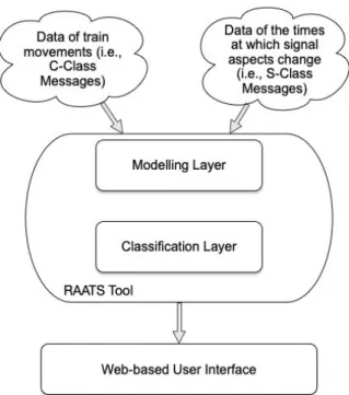
There are two layers in the kernel of the RAATS Tool: a modelling layer that models the scenario of a train approach towards a signal; and a classification layer that classifies the approaches into different classes (see Fig. 2).
Figure 2: Architecture of the RAATS tool
At the model layer, millions of records are processed and those which are related are selected and used to describe the circumstances of a train travelling through three sequential berths. The results from the first layer provide a foundation for the process in the classification layer. In the classification layer, each case of a train approaching a signal is classified into one of several classes based on the timing information of the train’s movement and the status of the corresponding signal.
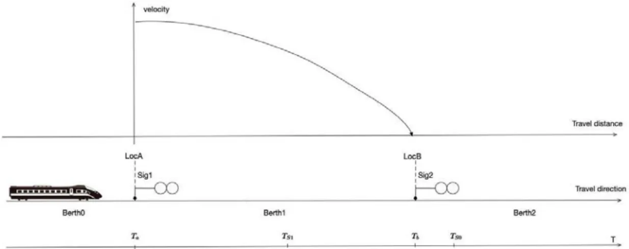
By processing live data streams from Network Rail, we are able to know each train’s movement at the berth level in terms of entry and exit timings. Figure 3 is an illustration of a typical scenario. A train travels into a berth of interest (Berth1 at LocA) at the time Ta. It is a red approach if the signal (Sig2) at the end of Berth1 is displaying a red aspect at time Ta. At time TS1, Signal Sig2 clears and the train moves towards the signal and leaves Berth 1 at LocB at time Tb. A short while later signal Sig2 changes back to red at time TS0.
Figure 3: A typical model of a train moving towards a signal with a red aspect
Based on the knowledge of typical approaches to red signals on the GB rail network and the timings Ta, Tb, TS1 and TS0, the model can estimate a train’s speed when entering the berth (Berth 1) and classify the train’s approach to a red signal (Sig2) into one of the following scenarios:
• NRA (Non-Red Approach): When the train enters the berth, the signal aspect at the end of the berth is showing a proceed (i.e., non-red) aspect.
• CSS (Cleared after Stopping at Signal): Signal clears after the train has come to a stand at the signal and the train departs immediately.
• CBD (Cleared Before Departure): Train enters the platform and stops at the red signal. This is a subset of the CSS category and is where a CSS approach occurs at a platform.
• CAS (Cleared on Approach to Signal): The signal is red when the train enters the berth but it clears (i.e. changes to a non-red aspect) before the train comes to a stand.
• PSS (Possibly Stopped at Signal): The signal possibly clears after the train has come to a stand and the train departs immediately. This class is the 'grey area' between the CSS and CAS classes and covers those train approaches which cannot be confidently classified as CSS or CAS using the currently available data.
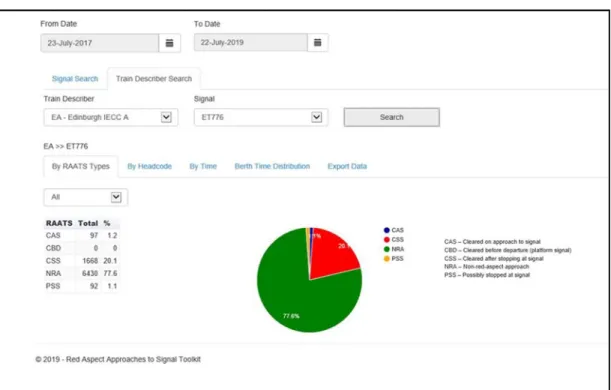
The tool currently exists as web-based application. Figure 4 shows an example of the current interface and some of the results that can be displayed on a signal basis.
Figure 4: RAATS tool interface
5. Current applications of RAATS
A. Using RAATS data to understand risk
The outputs from RAATS are vitally important in risk and safety analysis. They allow a better indication of the chance for a signal to be passed at red than any other normaliser (e.g., train miles, total number of trains passing a signal) that has been used to date. In addition, there are many risk models and tools currently in existence, not to mention the many assessments that have been undertaken that have utilised, or attempted to incorporate within them, parameters related to the red aspect approach to a signal. For such a key parameter, it is important to note that until recently only crude estimates of the
rates or proxies for them have been used as understandably no tool (until RAATS) was available to obtain them. This situation has mainly driven the development of the tool, but note that knowledge of red aspects is not limited to just risk and safety analysis, they also play an integral part in understanding train performance (punctuality and delay). This section of the paper will look at some of these applications in more detail and illustrate how the RAATS data is envisaged to be used and developed in the future.
B. Risk Modelling
Network Rail assesses the SPAD risk associated with every signal on the network using a process which examines the frequency and the potential consequences of passing that signal at danger. A tool has been developed, the Signal Overrun Risk Assessment Tool (SORAT), to undertake signal risk assessments. The risk assessment considers factors such as distance to a conflict point (such as a junction), train speed and passenger loading. This process does not currently incorporate any estimates for the number of red aspect approaches to a signal within the risk assessment; however, it aspires to do so if such information was readily available. Enabling this will improve the granularity of the modelling that the tool undertakes and allow better localisation and estimates of the relative level of SPAD risk at signals to be made.
Another application that will benefit from RAATS data is the RSSB Safety Risk Model (SRM) [7]. The SRM is a mathematical model of the risk arising from the operation and maintenance of the GB railway. It provides the GB rail industry with national estimates of risk through a series of models, some of which consider SPADs and the consequences that can ensue from them. Research is currently underway by RSSB (R&D project T1136 [14]) to look at redeveloping the model and investigating new techniques and ideas that can help improve and refine the risk estimates the model makes. One of the ideas that has been looked at is developing a SPAD Bayesian Network model that will enable a framework of causes, factors, attributes and conditions to be modelled. A demo model has been produced and RAATS data has been used as one of the inputs.
C. Human reliability quantification
A previous study [3] made an observation that signals with a high proportion of red aspect approaches actually have a relatively low chance of a SPAD occurring for each red aspect approach because drivers are accustomed to approaching the signal at red. Conversely, signals with a low proportion of red aspect approaches have a relatively high chance of a SPAD occurring when the signal is approached at red because drivers are not expecting a red signal. There is also the question of SPAD potential based on the frequency of red aspect approaches. Are signals with more red aspect approaches
proportionately more likely to have a SPAD event? It is likely to be a combination of the two factors, the frequency of red aspect approaches and the proportion of approaches to the signal that are red aspect approaches that influence the chance of a SPAD at the signal.
Initial analysis of the RAATS data has also highlighted that the type of train (e.g., express, stopping, empty coaching stock, freight etc) is also a factor that needs to be considered when calculating SPAD probability. The work raises the question of what is meant by SPAD probability, as it really depends on the context in which this is answered. On the one hand we can look at SPAD probabilities associated with different types of train approaches to a single signal, which could be further broken down by operator. Alternatively, looking at it another way, SPAD probability could be calculated from an operator’s perspective along a route, taking into consideration all of the train approaches to signals on a journey across all of the operator’s services.
6. Further applications of RAATS
There are a number of other potential uses of the underlying train TD data that RAATS is based on. The analysis has the potential to assist with understanding performance and capacity constraints on the network. This could be achieved by comparing the theoretical timetable against what actually occurs and assessing if there are areas where it could be optimised or designed better. TD data could also be used to identify changes, locally and nationally, in red aspect demands as a result of timetable changes or as a result of incidents causing disruption. This is particularly important when large scale changes are being made and an example of what happens when it goes wrong was widely reported in the British press over 2018 and led to an inquiry by the Office of Rail and Road [15].
Another use could be in understanding the routing of trains, the positions of points at junctions along with the frequency of their use. This is particularly useful in the context of a signal risk assessment where there are multiple conflict paths that a train could take in the event of passing it at danger. The RAATS data provides a way of calculating the probability that each route could be taken. It also provides a way of counting trains as they pass through the rail network and these statistics have a wide use in understanding usage and normalisation when making comparisons.
Further applications of the data might involve further algorithm development, particularly with regards the braking and acceleration profile of a train as it passes through the berth. The model is relatively simple at the moment, however it could be developed further, possibly by linking to other data on the train or external to understand where and for how long traction is taken or braking is made and then infer from this other metrics like track degradation, energy usage or emissions.
7. Future Development
D. Using RAATS in further big data analyses
RAATS data in itself provides useful information to understand the number of times a signal is approached at red. The main benefit of this data though will be in combination with other data sets, some of which are potentially very large (e.g. train recorder information, weather conditions, delay statistics etc). To make the sort of gains in safety improvement outlined at the start of the paper is likely to require ever more sophisticated and granular modelling techniques. The reason for this lies in the fact that economically viable and justifiable safety improvements tend to need to be identified at quite specific locations (e.g. a particular signal) rather than as a national policy (e.g. all signals). There are of course exceptions, and large-scale fitment of say a new train protection system or equivalent on the GB railway could potentially make a substantial difference, but it would be at cost and perhaps justified in terms of both safety improvement and other wider economic benefits. In terms of identifying improvements solely on a safety basis (and for which there is a legal requirement to do so), there is a need and an emphasis now to model at very specific locations, which in turn increases the amount of data that needs to be collected and the demands on the modelling framework to make sense of it. Utilising the principles of big data analysis and creating a model that has the capability of combining diverse and large data sets is at the forefront of the GB rail industry’s efforts to better understand SPAD risk.
In [16] a first attempt was made at such an approach, bringing together SPAD and RAATS data with signal asset data to assess the characteristics of the GB rail network potentially give rise to SPADs. This method offers some huge opportunity, as it facilitates an analysis framework to be set up where information at signals that have experienced a SPAD can be used to infer information about signals that have yet to experience a SPAD. On the GB rail network there are approximately 30,000 signals and each year around 300 SPADs occur [9]. A lot of these are at signals that have never seen a SPAD before and in some cases upon investigation some additional controls and risk mitigation can be identified to help prevent further occurrences. In the future the aim is to be able to do this pre-incident and use a big data approach to help prevent incidents before they occur by identifying classes of signal based on their characteristics that warrant some sort of intervention.
Some progress has been made in attempting to do exactly that. In the Tavison project
[17] the aim was to try and combine several related data sources (one of which was RAATS) to better understand SPAD risk. Other sources of data included the on-train data recorder (OTDR) and close call incident data within a graph database to assess where the network was vulnerable to SPADs manifesting. The work showed that it was indeed possible and developed a working framework, however it also highlighted that there are several obstacles to