High-Throughput Data Analysis: Application to Micronuclei Frequency and T-cell Receptor Sequencing

(1)

Virginia Commonwealth University

VCU Scholars Compass

Theses and Dissertations Graduate School

2015

High-Throughput Data Analysis: Application to

Micronuclei Frequency and T-cell Receptor

Sequencing

Mateusz Makowski

Virginia Commonwealth University, [email protected]

Follow this and additional works at:http://scholarscompass.vcu.edu/etd

Part of theBiostatistics Commons,Genetic Processes Commons, and theOther Immunology and Infectious Disease Commons

This Dissertation is brought to you for free and open access by the Graduate School at VCU Scholars Compass. It has been accepted for inclusion in Theses and Dissertations by an authorized administrator of VCU Scholars Compass. For more information, please [email protected].

Downloaded from

(2)

High-Throughput Data Analysis:

Application to Micronuclei Frequency

and T-cell Receptor Sequencing

A dissertation submitted in partial fulfillment of the requirements for the degree of Doctor of Philosophy at Virginia Commonwealth University.

by

Mateusz Makowski

B.S. Biology and Mathematics, Dickinson College, USA, 2007

Director: Kellie J. Archer, Ph.D., Professor, Department of Biostatistics

Department of Biostatistics Virginia Commonwealth University

Richmond, Virginia, USA August, 2015

(3)

Acknowledgements

I would like to thank my adviser, Dr. Kellie J. Archer, for her patience in guiding me through the process of my doctoral work. She has been a wealth of information and support and I could not have finished without her. I would like to thank my committee members Dr. Nitai Mukhopadhyay and Dr. Roy Sabo for their time, patience and feedback related to statistics. I would like to thank Dr. Amir Toor and Dr. Masoud Manjili for serving on my committee, providing data for my dissertation and most importantly providing background on the biological aspects of my dissertation.

I also would like to thank my peers in the Department of Biostatistics, we learned as much from each other as from our instructors. I would like to thank the administration of the department for helping guide me through the process as well.

I would like to thank my friends in Richmond, especially the tennis community, for keeping me from doing nothing but sitting in front of my computer. I would like to thank my undergraduate roommates, Andy and Andre, who have always managed to stay in touch despite the many miles separating us. They have always been a shoulder to lean on.

Lastly, but most importantly, I want to thank my family. First I would like to thank my mother, Urszula, for her love and support during this long process. I would also like to thank my dad, Sam, and brother, Marty, for being supportive as well. I would also like to thank all my extended family that always showed interest in my research and progress. Finally, I would like to thank my wife, Maunette, for her keeping me sane during this process and always being there for me. Thank you for being by my side for the last 11 years and the many years to come.

(4)

List of Tables

1 Table of Methods for Analyzing TCR Sequencing Data . . . 26

2 Median Perturbation Using Matched Donor Control . . . 37

3 Median Perturbation Using Mean Control . . . 38

4 Median Simpson’s Diversity . . . 44

5 Median Shannon Diversity . . . 46

(7)

6 Median Alpha Value . . . 51

7 Median of the logit transformed proportion of shared sequences . . . 53

8 Compositional Linear Model p-values . . . 70

9 Common V or J Gene Using Different Analyses . . . 72

10 Genes Identified as Associated with MN Count by both GMIFS and glmpath 91 11 Methylation Loci Identified as Associated with Bud Formation . . . 99

List of Figures

1 VDJ Recombination: A schematic of how separate V,D and J segments are recombined into a functional TCR protein (Adapted from Janeway et al. [2001]). 2 2 CDR3 Region: A diagram of where the CDR3 region occurs in a recombined VDJ segment. . . 3

3 TCR distributions: (A) Shows a typical Gaussian polyclonal distribution. (B) Shows a Gaussian distribution that is also polyclonal. (C) shows a non-Gaussian distribution that is monoclonal [Miqueu et al., 2007] with permission. 4 4 Spectratype Schematic Shows steps taken to run to generate spectratype data. (A) shows using electrophoresis to separate the mRNA by size. (B) shows measuring the band intensity. (C and D) show translating the band intensities into a distribution by size [Miqueu et al., 2007] with permission. . 4

5 Sequencing Assay Strategy SchmaticA generic TCRβCDR3 PCR prod-uct is shown. Primers include parts of the V and J segments and also the Genome Analyzer Cluster station (GA F and GA R). The NDN region rep-resents the CDR3 region. The primers were designed to capture just enough of the J and V segments to allow identification [Robins et al., 2012] with permission. . . 5

(8)

6 Reproducibility PlotsThe plots show frequencies of unique sequences from

different samples. . . 31

7 Distribution of perturbation from matched donor statistic for the 2

signifi-cantly different VDJ combinations. . . 36

8 Distribution of perturbation from mean donor statistic for the 3 significantly

different VDJ combinations. . . 37

9 Distributions of CDR3 lengths from VDJ combination TRBJ2-6 TRBV9

TRBD1-2 donors. . . 38

10 Distributions of CDR3 lengths from VDJ combination TRBJ2-6 TRBV9

TRBD1-2 recipients. . . 39

11 Distribution of CDR3 length for highest Oligoscore in GVHD group. . . 41

12 Distribution of CDR3 length for highest Oligoscore in No GVHD group. . . . 42

13 Distribution of Simpson’s Diversity Index statistic for the 5 significantly

dif-ferent VDJ combinations. . . 43

14 Distribution of Shannon’s Diversity Index statistic for the 6 VDJ combinations

having the smallest p-values. . . 46

15 CDR3 length distribution for each patient of VDJ combination: TRBJ2-1,

TRBV18, TRBD1-1. . . 48

16 CDR3 length distribution for each patient of VDJ combination: TRBJ1-2,

TRBV3-1, TRBD1-1. . . 49

17 Distribution of the non-parametric α statistic for the significantly different

VDJ combination. . . 51

18 Distribution of the logit transformed proportion of shared sequences for the 2

VDJ combinations having the smallest p-values. . . 53

19 Cluster Dendrogram of the 13 HSCT patients. . . 71

(9)

20 Number of Predictors Correctly Identified as Non-zero: This figure shows the distribution of the number of predictors correctly identified as non-zero over 100 simulations. There were 5 predictors had non-zero coefficients. Boxplots are separated by the type of distribution used to generate the data and number

of observations. . . 87

21 Number of Predictors Incorrectly Identified as Non-zero: This figure shows the distribution of the number of predictors incorrectly identified as non-zero over 100 simulations. There were 95 predictors that had coefficients set to zero. Boxplots are separated by the type of distribution used to generate the data and number of observations. . . 88

22 Accuracy of Count Predictions: This figure shows the distribution of the sum of residuals squared over 100 simulations using a learning data set and an independent test data set. Boxplots are separated by the type of distribution used to generate the data and number of observations. The results forglmpath with Gaussian family using an offset are not displayed because both values are above 50,000. . . 89

23 Histogram of MN Counts for cord blood data set. . . 92

24 Plot of actual MN counts versus predicted MN counts using GMIFS. . . 92

25 Plot of actual MN counts versus predicted MN counts usingglmpath. . . 93

26 Plot of actual MN counts versus predicted MN counts using glmpath using 17 non-zero coefficients. . . 93

27 Histogram of MN Counts for breast cancer data set. . . 97

28 Histogram of bud frquencies in the breast cancer data set. . . 98

29 Plot of actual MN counts versus predicted MN counts using GMIFS for breast cancer data. . . 98

(10)

Abstract

High-Throughput Data Analysis: Application to Micronuclei Frequency and T-cell Receptor Sequencing

by Mateusz Makowski

A dissertation submitted in partial fulfillment of the requirements for the degree of Doctor of Philosophy at Virginia Commonwealth University.

Virginia Commonwealth University, 2015

Major Director: Kellie J. Archer, Ph.D., Professor, Department of Biostatistics The advent of high-throughput sequencing has brought about the creation of an unprece-dented amount of research data. Analytical methodology has not been able to keep pace with the plethora of data being produced. Two assays, ImmunoSEQ and the cytokinesis-block micronucleus (CBMN), that both produce count data and have few methods available to analyze them are considered .

ImmunoSEQ is a sequencing assay that measures the β T-cell receptor (TCR)

reper-toire. The ImmunoSEQ assay was used to describe the TCR repertoires of patients’ that have undergone hematopoietic stem cell transplantion (HSCT). Several different methods for spectratype analysis were extended to the TCR sequencing setting then applied to these data to demonstrate different ways the data set can be analyzed. The different methods in-clude CDR3 distribution perturbation, Oligoscores, Simpson’s diversity, Shannon diversity, Kullback-Leibler divergence, a non-parametric method and a proportion logit transformation method. Herein we also demonstrate adapting compositional data analysis methods to the TCR sequencing setting. The various methods were compared when analyzing a set of 13 subjects who underwent hematopoietic stem cell transplantation. The eight subjects who developed graft versus host disease were compared to the five who did not. There was no little overlap in the results of the different methods showing that researchers must choose the appropriate method for their research question of interest.

(11)

The CBMN assay measures the rate of micronuclei (MN) formation in a sample of cells and can be paired with gene expression or methylation assays to determine association be-tween MN formation and other genetic markers. Herein we extended the generalized mono-tone incremental forward stagewise (GMIFS) method to the situation where the response is count data and there are more independent variables than there are samples. Our Poisson

GMIFS method was compared to a popular alternative, glmpath, by using simulations and

applying both to real data. Simulations showed that both methods perform similarly in

ac-curately choosing truly significant variables. However, glmpathappears to overfit compared

to our GMIFS method. Finally, when both methods were applied to two data sets GMIFS

(12)

1 T-Cell Receptors and the Adaptive Immune System

1.1 T-cell Biology

The adaptive immune system is responsible for recognizing foreign and self antigens and mounting the proper response. This is known as acquired immunity because the body “re-members” the specific antigen and can mount a quicker and more potent response each subsequent time the body encounters that antigen. T and B cells are responsible for main-taining an acquired immunity. T cells are a type of cell that maintains the body’s immunity by activating genes that create cell surface receptors that recognize foreign and self antigens. These genes and subsequently receptor proteins are passed on to future generations of cells

during cell division. T-cell receptors (TCR) are heterodimers that contain an α and a β

chain or a γ and a δ chain. The chains are made up of several different regions; a constant

region, a variable region, a transmembrane domain and a short cytoplasmic tail. Further,

the variable region of the β chain of TCR’s is made up of the variable (V), joining (J) and

diversity (D) gene segments [Robins et al., 2009, Rudolph et al., 2006].

T-cells are activated when the TCR recognizes an antigen bound to a major histocompat-ibility complex (MHC) molecule presented to it by an antigen presenting cell (APC) [Avent, 2012]. Once the antigen is recognized an immune response is launched. The first step in a memory response is to have a TCR that recognizes a specific antigen. Because there is a large diversity of antigens the human body can come in contact with, the immune system must have a way to generate a large diversity of TCR’s. Producing a large diversity of TCR’s is accomplished by a process called VDJ recombination (Figure 1). VDJ recombination is the joining of different gene segments to create unique amino acid sequences. Specifically, V, D and J segments that are spread across human chromosomes 2,14 and 22 are combined to make a unique VDJ combination.

In this review we are only interested in VDJ recombination of the β chain of TCR’s

(TCRβ). There are 52 known V gene segments, 2 D gene segments and 13 J gene segments

(13)

[Janeway et al., 2001] in the TCRβ chain. All possible VDJ combinations yield 13×2×52 = 1352 possible combinations. This is not a large variety and further diversity in TCR’s is added by the amino acid sequence encoded in the third complementary-determining region (CDR3) [Robins et al., 2009]. The CDR3 region occurs at the VDJ junction. As can be seen in Figure 2, this junction includes part of the V segment, all of the D segment and the J segment. The CDR3 region undergoes template-independent additions and deletions

of nucleotides during TCR gene rearrangement. This greatly increases TCRβ diversity.

Arstila et al. [1999] reported estimates of 106 unique TCRβ CDR3 sequences per person.

By measuring the abundance of each clone a better understanding of the human immune response can be gained [Carlson et al., 2013].

Figure 1: VDJ Recombination: A schematic of how separate V,D and J segments are re-combined into a functional TCR protein (Adapted from Janeway et al. [2001]).

(14)

Figure 2: CDR3 Region: A diagram of where the CDR3 region occurs in a recombined VDJ segment.

1.2 Technology for Measuring TCR

β

Clones

Historically, measuring TCR abundance was done by spectratype analysis, a process that measures relative abundance of TCR clones. Unfortunately, spectratyping can only distin-guish a particular V, D or J segment. For a specific V or J gene the clones are separated by size rather than sequence [Kepler et al., 2005]. This is useful in general terms to monitor TCR diversity. A more detailed review of spectratype analysis methodology can be found in section 1.6.

Figure 4 shows a schematic of how spectratyping assay is done. First a sample is collected

and the T-cells are isolated. PCR is then used to replicate only a specific TCRβ gene segment

(V, D or J) by using primers specific to a TCRβ segment. The mixture of CDR3 region

clones is then separated by size using electrophoresis. The results are then presented on histograms with number of TCR’s at each specific size [Kepler et al., 2005]. Note that spectratyping separates CDR3 regions by size, if two different CDR3 sequences are of the same length they will be counted in the same bin. Figure 3 shows examples of some common CDR3 length distributions that result from spectratype analysis.

Recent improvements in sequencing technology allow for much greater detail in measuring TCR diversity [Robins et al., 2009]. Adaptive Biotechnologies developed an immune profiling assay, ImmunoSEQ, that uses parallel sequencing to capture 48 possible V segments, 13 J segments and 2 D segments by simultaneous use of PCR primers for each segment [Robins et al., 2009]. This allows for simultaneous sequencing of a large portion of the human T-cell

(15)

Figure 3: TCR distributions: (A) Shows a typical Gaussian polyclonal distribution. (B) Shows a non-Gaussian distribution that is also polyclonal. (C) shows a non-Gaussian distri-bution that is monoclonal [Miqueu et al., 2007] with permission.

reportoire. The assay maximizes throughput by only amplifying and sequencing the region of the TCR that contains the CDR3 region. This allows for short reads, 60 nucleotides in length, to be used to identify each sequence. Further, the assay can be used on both cDNA and genomic DNA [Robins et al., 2009]. Recently, Adaptive Biotechnologies developed a new method to correct for PCR bias caused by using so many different primers [Carlson et al.,

2013]. By using sequencing, researchers can distinguish TCRβ clones down to the level of

unique CDR3 clones.

Figure 4: Spectratype SchematicShows steps taken to run to generate spectratype data.

(A) shows using electrophoresis to separate the mRNA by size. (B) shows measuring the band intensity. (C and D) show translating the band intensities into a distribution by size [Miqueu et al., 2007] with permission.

(16)

Figure 5 shows a schematic of a generic PCR product used by the ImmunoSEQ assay.

13 reverse J primers and 48 forward V primers were designed to capture 13×2×48 = 1248

possible VDJ combinations. All sequences contain small portions of the V and J segments as well as the CDR3 region. This allows not only for gene segment family identification but also unique CDR3 identification.

Figure 5: Sequencing Assay Strategy SchmaticA generic TCRβ CDR3 PCR product is

shown. Primers include parts of the V and J segments and also the Genome Analyzer Cluster station (GA F and GA R). The NDN region represents the CDR3 region. The primers were designed to capture just enough of the J and V segments to allow identification [Robins et al., 2012] with permission.

1.3 ImmunoSEQ Precision, Accuracy and Sensitivity

Robins et al. [2012] conducted experiments using the ImmunoSEQ platform to determine its precision, accuracy and specificity. Samples containing spiked-in clones of known con-centration ranging from 10 to 100,000 cells per million were created. The experiments show that the assay can detect clones reliably at a level of one cell per 100,000.

The spike-in experiments were designed to test the assay’s accuracy and sensitivity. Dif-ferent mixtures of five CD4+ T-cell clones specific for GAD65 were spiked into a background of one million CD4+ T cells. Three different mixtures were made using these five clones. Two other T-cell clones that targeted tumor-associated NY-ESO-1 antigen were also used. These were spiked directly into autologous peripheral blood mononuclear cells instead of sep-arated cells. The titrations that were used were 1/100,000, 1/10,000, 1/1000 and 1/100. The different mixtures were then sequenced using the method described in section 1.2. The raw data results in counts for each unique CDR3 region. Finally, a nearest neighbor alogrithm was used to merge closely related sequences to remove PCR and sequencing errors. The

(17)

cessed data were then used to estimate the frequencies of each spiked in clone. The results show that 6 out of 7 of the clones had an observed frequency very close to the expected. The 7th clone was not detected at all because it contained a 16 nucleotide deletion and the assay is designed to capture all clones with deletions of 14 nucleotides or fewer (this deletion length

accounts for 99% of TCRβ’s) [Robins et al., 2012]. Thus, the assay is extremely accurate in

detecting clones even at low concentrations.

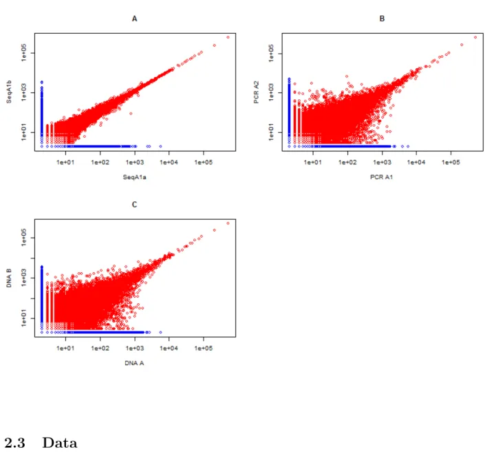
Finally, the reproducibility of the assay was tested. Blood was drawn from one subject and DNA was extracted two independent times (DNA A and DNA B). The DNA A sample was then PCR amplified two independent times (PCR A1 and PCR A2) while the DNA B sample was only PCR amplified once (PCR B1). Finally, sample PCR A1 was sequenced two independent times (SeqA1a and SegA1b) while samples PCR A2 and PCR B1 were only sequenced once (SegA2a and SeqB1a). Robins et al. [2012] showed that sequencing from the the same PCR library is highly reproducible. Robins et al. [2012] showed that sequencing from different PCR libraries is also reproducible but not quite as much. Finally, Robins et al. [2012] showed that sequencing different DNA extractions is also reproducible but again not quite as much as the other two conditions. In the different blood draw samples, approximately 55 % of all reads were obtained from shared sequences. This is probably due to a blood draw being a finite sample so each one is a random subset of all clones [Robins et al., 2012].

1.4 Unseen Species and Estimating the TCR

β

Repertoire using

ImmunoSEQ data

1.4.1 Unseen Species Problem

The unseen species problem is one that has been tackled several times over the years. Efron and Thisted [1976] described a method for estimating unseen species. The unseen species problem was first considered in ecology, where researchers needed to estimate the number

(18)

of different types of species in a given area assuming they could not sample every organism.

That is, if a given area is sampled and n species are found, the unseen species problem

is to estimate how many more unique species are in the area that were missed by the sample. A different application that may help elucidate this concept is to consider William Shakespeare’s vocabulary. Given all the different words he used in his writing, we may want to estimate how many words Shakespeare actually knew assuming he did not use all of them in his works. The unseen species estimation problem in this case is, if a new work from Shakespeare is found, to estimate the number of new words not used in his previous works. Shakespeare’s works are comprised of 884,647 total words, 31,534 of which are unique [Efron

and Thisted, 1976]. Letnxrepresent the number of words occuringxtimes (x= 1 to∞). The

method described by Efron and Thisted [1976] says, assuming the new works are the same size as the old, 11,460 new words would be expected. The basic model uses an empirical Bayes approach and is described later in this section. Recently, this method has been modified to genome sequencing [Ionita-Laza et al., 2009] and T-cell receptor sequencing [Robins et al., 2009].

The methodology described by Efron and Thisted [1976] can be thought about using

species trapping terminology. Suppose there existSspecies and after trapping for one unit of

time we capturexsmembers of speciess. We then assume thatxs has a Poisson distribution

with a mean of λs. It is convenient to consider the time period to be [−1,0] and we wish to

extrapolate to a time t in the future. Let xs(t) be the number of times species s appears in

[−1, t].

Before moving on, it is of relevance to review the Poisson distribution. The Poisson distribution is a widely used discrete distribution for modeling count data. For example, the Poisson distribution can be used to model the number of occurences of a phenomenon in a given time period [Casella and Berger, 2002]. In this case, the number of species seen in a given area in a given time period. The basic assumption the Poisson distribution is built on is that the probability of occurence is proportional to length of waiting time. So the Poisson

(19)

distribution has one parameter λ, sometimes called the intensity parameter [Casella and

Berger, 2002]. A random variable, X has a Poisson(λ) distribution if

P(X =x|λ) = e −λ_λx

x! , x= 0,1,2, ...

where the_E(X) = λ and var(X) = λ. Two useful characteristics of the Poisson distribution

are that the sum of independent Poisson random variables is itself Poisson distributed and a Poisson random variable conditioned on a sum of Poisson variables is binomial. More formally,

Theorem 1. If X ∼ P oisson(θ) and Y ∼P oisson(λ) and X and Y are independent, then X+Y ∼P oisson(θ+λ) [Casella and Berger, 2002].

The Poisson distribution assumption implies, using Theorem 1, that xs(t) is distributed

Poisson(λs(1+t)). Furthermore, we can say that

xs|xs(t)∼Binomial xs(t), 1 1 +t . Proof. Assuming xs ∼P oisson(λs) Then xs(t)∼P oisson(λs(1 +t))

given there are 1 +t time points in the [−1, t] and by Theorem 1. Next to show xs|xs(t) is

binomially distributed, letxs(t) =xs+xs(t−1) where xs(t−1) does not include the interval

[−1,0]. Note that Pr(xs(t−1) = xs(t)−xs | xs) = Pr(xs(t −1) = xs(t)−xs) because

xs(t−1) does not include the interval [−1,0] and therefore is not dependent on xs. So we

(20)

Pr(xs |xs(t)) = Pr(xs, xs(t) =xs+xs(t−1)) Pr(xs(t) = xs+xs(t−1)) = Pr(xs) Pr(xs(t−1) =xs(t)−xs|xs) Pr(xs(t) = xs+xs(t−1)) = Pr(xs) Pr(xs(t−1) =xs(t)−xs) Pr(xs(t) = xs+xs(t−1)) = exp(−λs)λ xs s xs! × exp(−λst)(λst) xs(t−1) xs(t−1)! × xs(t)! exp(−λs(1 +t))(λs(1 +t))xs(t) = xs(t) xs exp(−λs)λxssexp(−λst)(λst)xs(t)−xs exp(−λs(1 +t))(λs(1 +t))xs(t) = xs(t) xs λxs s (λst)xs(t)−xs (λs(1 +t))xs(t) = xs(t) xs λxs s (λst)xs(t)−xs (λs(1 +t))xs(t)−xs+xs = xs(t) xs 1 1 +t xs t 1 +t xs(t)−xs = xs(t) xs 1 1 +t xs 1− 1 1 +t xs(t)−xs

This is a binomial distribution with n =xs(t) and p= ₁₊1_t.

Let G(λ) be the empirical cumulative distribution function of λ1, ..., λS. If nx is the

number of species observedx times in [−1,0], let

ηx =E(nx) = S ∞ Z 0 (e −λ_λx x! )dG(λ), (1)

where λ is the λ associated withG(λ). Next, let ∆(t) be the expected number of species in

(0, t] but not in [−1,0]. Note that using equation 1 the probability of not seeing a species

in a given interval (observing x = 0) is given by exp(−λ). Likewise, the probability of not

seeing a species in the interval [−1,0] is exp(−λ) so that the probability of seeing a species in the interval (0, t] is 1−exp(−λt). Thus,

(21)

∆(t) =S

∞ Z

0

exp−λ(1−exp−λt)dG(λ).

To estimate ∆(t) we can use a Taylor series expansion of 1−exp−λt,

1−exp−λt =λt−λ

2_t2

2! +

λ3_t3

3! −...

and substituting the right hand expression into the expression for ∆(t) we get

∆(t) = S ∞ Z 0 exp−λ(λt− λ 2_t2 2! + λ3_t3 3! −...)dG(λ) which can be rexpressed as

∆(t) =S ∞ Z 0 exp−λλt 1! − exp−λλ2t2 2! + exp−λλ3t3 3! −... dG(λ).

Substituting equation 1 into the right hand side we get

∆(t) = η1t−η2t2+η3t3−...

Thus an estimate for ∆(t) is

ˆ

∆(t) =n1t−n2t2+n3t3−. . . .

This estimate works well when t = 1 but when t > 1 the tx _{values cause wild oscillations}

which may cause convergence issues. Euler’s transformation is one way to force the series to converge. Euler’s transformation is defined [Knopp, 2013] as

∞ X k=0 (−1)kak = ∞ X n=0 ∆na0 2n+1 where

(22)

∆ka0 = k X m=0 (−1)m k m ak−m

which is the form that the unseen species estimate takes. That is

∞ X k=0 (−1)kak = ∞ X x=1 (−1)x+1ηxtx.

Application of this transformation is discussed further in section 1.4.2.

1.4.2 TCRβ CDR3 Diversity

Robins et al. [2009] used the unseen species method described in section 1.4.1 to estimate

the human TCRβ repertoire. Using the same terminology as in 1.4.1, the total number of

unique TCRβ CDR3 sequences in the reportoire is represented by S. Let xs represent the

number of a specific CDR3 sequence,s, observed in an experiment. Further, assuming T-cells

circulate freely in the blood, it can be assumed that each CDR3 count, xs, is distributed

P oisson(λs). Let xs(t) represent the number of times a CDR3 sequence was observed in

sequencing experiment t and every previous experiment. Here, t represents the numbered

experiment, 1,2, ..., that was sequenced. Finally, let nx represent the number of CDR3

sequences observed exactly x times. Once again, we need to estimate ∆(t), the number of

CDR3 sequences expected to be observed in all sequencing experiments except the first one,

t = 1. This gives us an estimate of the total number of unique CDR3 sequences that could

be observed in one subject. Once again the estimate for ∆(t) is

ˆ

∆(t) =n1t−n2t2+n3t3−...

By letting t = u

2−u the following relationship is derived using Euler’s transformation from

section 1.4.1

(23)

∞ X x=1 (−1)x+1ηxtx = ∞ X y=1 ξyuy where ξy = ∞ X x=1 y−1 x−1 (−1)x+1 2y ηx = 1 2yδ y₍_η 1) and δ0 =η1, δ1 =η1 −η2, δ2 =η1−2η2+η3, . . . . Let ∆x0₍_t_{) =} ∞ X x=1 (−1)x+1ηxtx ∆x0₍_u_{) =} ∞ X y=1 ξyuy ∆(t) = lim x0→∞ ∆x0₍_t₎ ∆(u) = lim x0→∞ ∆x0₍_u₎_.

By definition ∆(t) = ∆(u) if both limits exist. Here ∆x0₍_u_{) converges much more quickly to}

the common limit [Efron and Thisted, 1976]. We can estimate ξy by substituting nx for ηx

and then estimate ∆(t) using

∆x0₍_u_{) =} ∞ X y=1 ξyuy = x0 X y=1 1 2yδ y₍_η 1)uy, u= 2t 1 +t.

Using the results from their sequencing experiments, Robins et al. [2009] estimated the

human TCRβ repertoire to be 105 CDR3 sequences. This result is similar to that obtained

(24)

1.4.3 Models for Estimating Population T-cell Diversity

Section 1.6 describes several T-cell receptor analysis methods in detail. This section will briefly describe several other methods present in the literature. Specifically, models to esti-mate overall T-cell diversity rather than just sample T-cell diversity will be presented.

Sep´ulveda et al. [2010] described a series of Poisson abundance models that can be used

to estimate the diversity in the original T-cell population. The clonal size distribution can be described by the following Multinomial law

P [mx|D,η] = D! (D−M) n Q x=1 mx! p_η(0)D−M n Y x=1 p_η(x)mx, (2)

where D is the number of distinct clonotypes in the population which is the population

diversity in this case. mx is the number of clonotypes withxcopies in the sample andpη(x)

is the probabilty of a clonotype being sampled x times and is described by a model with

parameter vector η. M is the sample diversity and n is the sample size. By assuming pη

follows a Poisson distribution, one can obtain the class of Poisson abundance models. The simplest Poisson abundance model is assuming a homogeneous Poisson distribution for all clonotypes. That is

pλ(x) = e−λλx

x! (3)

whereλis the sampling rate. This can then be plugged back into equation 2 forp_η. However,

it is very simplistic to assume all clonotypes have the same sampling rate. Thus, different

distribution can be obtained by applying a distribution to λ.

The first model to consider is the Poisson-Gamma model where λ follows the Gamma

distribution. This assumes clonotypes have different sampling rates based on their clonal size (the number of times a clonotype appears in the sample). By mixing equation 3 with a

Gamma distribution for λ we get

(25)

pα,β(x) = Z ∞ 0 e−λ_λx x! βα_λα−1_e−λβ Γ(α) dλ = Γ(x+α) Γ(x+ 1)Γ(α) β β+ 1 α 1 β+ 1 x , (4)

where α and β are the shape and scale parameters of the Gamma distribution.

Another model is the Poisson-lognormal model. This model assumes that λ follows a

lognormal distribution with parametersµandσ2_{. Using this model the sampling probability}

is pµ,σ2(x) = Z ∞ 0 e−λ_λi x! e(log2λσ−2µ)2 √ 2πσ2 dλ. (5)

This does not have a closed form and a numerical algorithm can be used such as the Newton-Raphson to calculate the probabilities.

The final model assumesλfollows an exponential distribution with paramterµ=e−ω_/₍₁₋

e−ω_{). Further,} _ω _{follows an exponential distribution with parameter} _ρ_{. Thus we get the}

fol-lowing sampling distribution

pρ(x) =ρ

Γ(x+ 1)Γ(ρ+ 1)

Γ(x+ρ+ 2) . (6)

Using the sampling probability equations, the diversity, D, can be estimated by maxi-mizing equation 2. Rempala et al. [2011] and Greene et al. [2013] expand these models to the multivariate setting to estimate population diversity. To choose the model that best fits the data goodness of fit tests can be computed such as the Pearson chi-squared test and AIC measure. Once an appropriate model is chosen, reportoires can be compared. The diversities can be compared by tests such as the Chi-squared or Kolmogorov-Smirnov tests. Because these tests are very sensitive to sample size, Mehr et al. [2012] suggest using machine learning methods such as repoirtoire clustering by similarity.

(26)

1.5 Application of TCR

β

Studies

1.5.1 Hematopoietic stem cell transplantation

Hematopoietic stem cell transplantation (HSCT) is used to treat hematological disorders such as blood cancers. The procedure involves replacing diseased host cells with healthy donor cells. A result of this procedure is graft-versus-tumor effect (GVT), which is when the reconstituted T-cells recognize the blood cancer and mount an immune response. Conversely, the reconstituted T-cells can recognize the new host and mount an autoimmune response known as graft-versus-host-disease (GVHD) [Avent, 2012]. Because GVHD is potentially lethal, it is extremely important to match donors to recipients to minimize the risk of donor

T-cells recognizing the recipients cells. The ability to measure TCRβ clone abundance can

greatly help in understanding the immune system’s requirement for initiating GVT versus GVHD.

1.5.2 Case Studies

Several studies have used the ImmunoSEQ assay to describe the T-cell repertoire in a variety of circumstances such as monitoring minimal residual disease (MRD), measuring diversity pre- and post-treatment and describing the T-cell repertoire during viral infection. This section will briefly describe six studies that have utilized the ImmunoSEQ assay.

Weng et al. [2013] studied the ability of high-throughput sequencing to monitor MRD in T-cell lymphoma patients. Samples from 10 patients were examined using the ImmunoSEQ assay. Tumor clones were identified prior to HSCT treatment and monitored using high-throughput sequencing. By using the ImmunoSEQ, Weng et al. [2013] were able to monitor recurrence of tumor clones that were a precursor of disease relapse using plots of percentage of malignant clone. Spike-in experiments were also performed that showed the assay could detect tumor clones with a sensitivity of 1:150,000.

Cooper et al. [2013] studied howBRAF inhibition affects the T-cell repertoire in patients

(27)

with metastatic melanoma. Serial biopsies from 8 patients were sequenced prior to treatment and 10-14 days after treatment using the ImmunoSEQ assay. T-cell diversity was calculated

pre- and post-treatment and the study found that treatment withBRAF inhibitors (BRAFi)

resulted in an increase in T-cell diversity in 7 out of 8 patients. The study also found that approximately 80% of the clones found in patients post-treatment were not present before treatment suggesting BRAFi treatment results in an influx of T-cells. Finally, the study found that the proportion of dominant clones present both pre- and post-treatment had an association with patient outcome. Patients with a high-proportion of pre-existing clones post-treatment had a better clinical outcome. It was unclear what specific statistical tests were performed.

Robert et al. [2014] also studied patients with metastatic melanoma but investigated treatment with drugs that inhibit cytotoxic T-lymphocyte-associated protein 4 (CTLA4) instead of BRAFi. CTLA4 inhibition can result in tumor remissions due to a T-cell response but this response has not been fully described. This study had two major conclusions. First, T-cell diversity increases post-treatment but does not seem to be related to the patients’ ability to fight cancer. Diversity was calculated using the Shannon diversity index which is defined as H =− L X i=1 pilog(pi) (7)

where pi is the probabiltiy of CDR3 length i. Second, patients with toxicity had a

signifi-cantly higher number of unique productive sequences after treatment. Because the authors had a large enough sample the Wilcoxon signed-rank test was used to compare diversity mea-sures pre- and post-treatment. The authors concluded that these results point to a general activation of the immune system rather than a specific anti-cancer immune response.

Muraro et al. [2014] studied the T cell repertoire post-HSCT in 24 multiple sclerosis (MS) patients. HSCT can be used as a way to reset the immune system in MS patients that have autoimmune disease (an organisms immune response to its own cells). The end point

(28)

of interest is a non-autoimmune repertoire. Samples were sequenced prior to treatment, two months after treatment and one year after treatment. The study found that patients that had a higher T-cell diversity at two months had a better clinical outcome. In this case diversity was the percentage of T cell repertoire that the top 100 clones included. It was unclear what statistical tests were performed to test for differences.

Finally, Zhu et al. [2013] and Neller et al. [2012] used the ImmunoSEQ assay to examine the T-cell repertoire in patients with herpes virus infection. Both studies showed that virus specific clonotypes are persistent in the patient’s T-cell repertoire. This suggests that there is a mechanism to promote a prompt response to viral recurrence.

1.6 Overview of Statistical Methods for CDR3 Data

Spectratype analysis is universally accepted as a procedure to monitor and calculate CDR3 length distributions. However, no agreement has been reached on a method to statisti-cally compare individual repertoires. There are two major hurdles when analyzing CDR3 spectratype data. The first is extracting information from each CDR3 distribution and the second is integrating all of the information from all the CDR3 distributions [Miqueu et al., 2007]. Initially, spectratype analysis was done by “eye-balling” the distribution and plac-ing it into a descriptional category. However, this methodology suffers from variation due to researchers having different ideas about which categories different distributions should fit into. Visual inspection and categorization is also an extremely time consuming method. Hence, researchers have used several computational methods to describe CDR3 distributions. Gorochov et al. [1998] described a method for measuring CDR3 distribution perturbation from a control distribution. This method is applied to T-cell repertoires during progression

of AIDS and describes the distributions as a whole. Collette et al. [2003] took this a step

further and described an OligoScore which describes each peak individually. This method can be used to identify recurrent peaks in different samples. Venturi et al. [2007] adapted a method from ecology called Simpson’s diversity index to measure the diversity in a CDR3

(29)

distribution. This method was applied to assess the T-cell repertoire recovery after HSCT by van Heijst et al. [2013]. All these methods assign scores to which statistical methods can then be applied. Kepler et al. [2005] described a statistical method that used the Kullback-Leibler divergence as a measure of how different CDR3 length distributions are from each other. Most recently, Bolkhovskaya et al. [2014] described a non-parametric method for comparing TCR distributions. In the following subsections each method is clearly described.

1.6.1 CDR3 Distribution Perturbation

The CDR3 length distribution measure was applied to measure T-cell repertoires during pro-gression to AIDS. This is a measure of how different TCR distributions are from each other. Gorochov et al. [1998] used data that was translated into a probability distribution from Immunoscope analysis. The area under each peak was measured to calculate a probability using the following formula

pi = Ai P i Ai (8)

whereAis the area under each peak (CDR3 length) and i= 1, . . . , LwhereLis the number

of amino acid lengths in the data. Modifying this notation, let pf_ik represent the probability

of peak i of TCRβ family f (VDJ combination) from sample k. The method then calls for

a control distribution for each TCRβ family. This was done by taking the average of the

control samples denoted by

pf_ic=X

k∈c pf_ik

|c| (9)

where c represents the indices of the control samples and |c| is the cardinality of c. The

perturbation of each peak from the control for sample k is then defined as

(30)

The sum of the absolute value of the peak perturbations is then

Df_k = 100×X

i

|D_ikf|

2 (11)

for sample k and TCRβ family f which yields an overall measure of perturbation for that

TCR profile in percentages for each TCRβ family. This is the generalized Hamming distance

and measures the distance between two strings of equal size. This measure ranges from 0 to 100 where 0 represents no difference from the control and 100 represents no overlap with the

control distribution. A further measure of overall perturbation for a sample k is defined as

Dk= F X f=1 D_kf F (12)

where F is the number of TCRβ families.

Different statistical tests can then be applied to the measures of perturbation to compare different groups. Gorochov et al. [1998] chose to use the Wilcoxon Rank sum test to compare groups. However, depending on sample size and distributional assumptions, a t-test may be appropriate as well. The the null hypothesis for this test, assuming a Gaussian distribution,

would be that the mean Dk is the same across all groups and the alternative hypothesis

is that at least one group’s mean is different. The hypotheses would be the same when

using D_kf except there would be many tests done, one for each TCRβ family. In this case

a multiple comparisons adjustment needs to be applied. For a more detailed discussion of multiple comparisons see section 1.6.8.

1.6.2 OligoScores

Collette et al. [2003] described a score to measure each peak within a group. The OligoScore

is defined for the ith _{peak of the} _kth _{sample as}

OligoScore(i) = exp(1)× N v u u t N Y k=1 pikexp(−nk) (13) 19

(31)

where pik is probability of the ith peak for the kth sample (as described in section 1.6.1),

nk is the number of peaks in each sample and N the number of samples [Collette and Six,

2002]. This score gives a measure of each peak within a group for each TCRβ family, f.

Oligoscores can be interpreted as a score that measures if the distribution has a major peak or not (higher scores mean a peak is major). Collette and Six [2002] did not do any hypothesis testing and instead ranked all oligoscores within each group. The highest oligoscore peaks were then looked at graphically. This score can be adapted to compute peaks for each VDJ combination.

1.6.3 Simpson’s Diversity Index

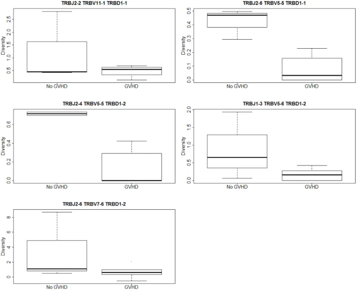
Slow T-cell recovery and low TCR diversity are risk factors for infection, cancer relapse and graft-versus-host-disease (GVHD) after hematopoietic stem cell transplantation (HSCT) [van Heijst et al., 2013]. See section 1.5.1 for a detailed description of GVHD and HSCT. Hence, measuring TCR diversity post-HSCT is an important way to monitor patient health. van

Heijst et al. [2013] suggested using the inverse Simpson’s diversity index (_D1

S). This measure

ranges from 1 to∞ where 1 is no diversity and∞is high diversity. The Simpson’s diversity

index in terms of TCR diversity using unique CDR3 length is the probability that any two TCR’s chosen at random from the sample will have different CDR3 lengths and is defined as DS = 1− L X i=1 nikf(nikf −1) nkf(nkf −1) (14)

wherenikf is the size of theith TCR CDR3 length (the number of copies of each TCR within

a CDR3 length and equivalent to the peak described in section 1.6.1) for the kth _{sample in}

TCRβ family, f. L is the number of different TCR CDR3 lengths in the sample and nkf is

the total number of TCR sequences sampled in sample k of TCRβ family, f. The diversity

index is computed for each TCRβfamily. This measure can then be used to compare groups

(32)

each VDJ combination.

van Heijst et al. [2013] were not interested in comparing groups but time points. Using paired t-tests they found the patient TCR diversity did not change over time. However, using correlations they did find that the composition of the TCR distribution changed drastically. For example, the dominant peak from one time point to the next could be completely different depending on what antigens the patient was in contact with recently.

1.6.4 Kullback-Leibler Divergence Method

Kepler et al. [2005] described this method directly for spectratype data which results in relative abundance measures as described in section 1.2. Let’s consider the multinomial

distribution in terms of CDR3 length distribution. In this case, L is the number of unique

CDR3 lengths, qis a vector of probabilities of each CDR3 length occuring,mi is the number

of counts of the ith CDR3 length and nk is the total number of counts within a sample.

Thus, the probability mass function (pmf) of the relative abundance of the lengths of CDR3 clones, p= m_n is fp(p|nk,q) =nkL−1Cnk(nkp) L Y i=1 qpink i , (15)

whereCn_k(nkp) is the multinomial coefficient andqis a vector of probabilities corresponding

to each category i. Cnk(nkp) = Γ(nk+ 1) L Q i=1 Γ(nkpi+ 1) (16) for L P i=1

nkpi =n and zero otherwise.

The Stirling approximation can then be applied to the multinomial coefficient to simplify its form assuming that for each i,nkpi is large enough.

(33)

logCnk(nkp) = log Γ(nk+ 1)− L X i=1 log Γ(pink+ 1) (17) = L X i=1 −nkpilogpi− 1 2logpi − L−1 2 log 2πnk+O( 1 nk ) (18)

Plugging this back into the pmf for p we get

fr(p|nk,q) = n(_kL−1)/2e−nkD(p;q) p (2π)L−1_ΠL i=1pi δ(0) (19)

where δ is the Dirac delta, p.= Σipi and D(p;q) is the Kullback-Leibler divergence.

D(p;q) = ΣL_i₌₁pilog pi qi

(20)

where p.=q.= 1.

To determine the distribution of the Kullback-Leibler divergence we can apply a cumu-lative generating function method where

h(s) = log Z dLpesD(p;q)fr(p|nk,q) (21) =−λlog(1− s nk ) (22)

This is the cumulative generating function of a gamma random variable withλ= (L−1)/2

and scale = _n1

k. The the distribution of the Kullback-Leibler divergence is given by

fD(D|nk) = n λ k Γ(λ)D λ−1 e−nkD ₍₂₃₎

Using the above derivations we can compare group distributions of the CDR3 length. We

(34)

hypothesis is that the distribution of CDR3 lengths is identical in all groups.

Let pijk represent the relative frequency counts of CDR3 length i = 1, ..., L, where j =

1, ..., G represents the group and k = 1, ..., nij the kth subject of the jth group for CDR3

length i. Then the mean of group j for CDR3 length i is defined as

¯ pij. = 1 ni nj X k=1 pijk (24)

whereni is the number of counts of CDR3 lengthiandnj is the number of subjects in group

j. If Gis the number of groups then the grand sample mean is

¯ pi.. = 1 n. G X j=1 nipij. (25)

where n. is the total number of subjects.

If we denote pjk as the vector that has componentspijk we can partition the total

diver-gence as Dtot = X j X k D(pjk;q) (26) =X j X k [D(pjk;¯pk.) +D(¯pk.;¯p..) +D(p¯..;q)] (27)

Under the null hypothesis that q is the same in all groups the expected values of the

partitioned divergences are

E[D(pjk;p¯k.)] = L−1 nk (1− G−1 n. ) (28) E[D(¯pk.;¯p..)] = L−1 nkn. (1− 1 G) (29) E[D(p¯..;q)] = L−1 n.nk (30) 23

(35)

Finally, because the divergences are distributed Gamma, the following statistic is asymptot-ically distributed as Fisher’s F with (L-1)(G-1) numerator and (L-1)(n.-G+1) denominator degrees of freedom under the null hypothesis.

F = (n.−G+ 1)ΣkD(p¯k.;¯p..) (G−1)ΣjkD(pjk;¯pk.)

(31) Notice that the numerator is a between group divergence and the denominator is within group divergence. This is analogous to the typical ANOVA test. This statistic can be used to compare different groups of subjects that have TCR data collected for them at each VDJ

combination, f.

1.6.5 Non-parametric Method

Bolkhovskaya et al. [2014] described a non-parametric method for assessing the TCR length distribution. To incorporate statistical uncertainty, a non-parametric kernel distribution

estimator is constructed for the cumulative frequency distribution, Ff(p∗)≡Prob(p≥p∗)

ˆ Ff(p) = 1 L L X i=1 Φ(p−pi), (32)

where L is the number of TCR lengths, pi is the frequency of each TCR CDR3 length, p is

a pre-chosen frequency value and Φ(·) is the cumulative normal distribution with mean zero

and standard deviation

σpi = " _S X s=1 σ2_p_i_,s #12 (33)

whereσ_p2_i_,s is the standard deviation present at each ofS steps of repertoire profiling. Three

steps (S) during the sampling process that add to statistical error are sampling T-cells, PCR and sequencing. Each of these steps introduce variation to the final TCR frequency. Bolkhovskaya et al. [2014] assume the sampling process at each step takes on a binomial distribution so

(36)

σ2_p

i,s =

s

pi(1−pi)

Ns (34)

where Ns is the total number of samples at step s. However, this variation can only be

measured at the sequencing stage so S = 1. From here the probability density distribution

can be estimated by

ˆ

W(p) = − d

dp = ˆFf(p). (35)

Finally, the upper 95% confidence interval can be computed using

p0 = 1−(1−0.95)z, z = S X s=1 1 Ns . (36)

Bolkhovskaya et al. [2014] applied this method to patient data and found thatFf(p) follows

a power law decay

Ff(p)∝pαi. (37)

The power law represents a relationship between two variables where one variable varies as the power of another. It can be seen in scenarios where a few values dominate. Many times a TCR CDR3 length distribution is dominated by one or two lengths. Thus, the power may be an appropriate way to compare TCR CDR3 length distributions between groups. This

can be done by calculating and comparing α values between groups.

1.6.6 Proportion Logit Transformation

The proportion of shared sequences between donor and recipient can be considered as a

measure of how closely the donor and recipient are matched. The question posed is if

there is a difference in the proportion of shared sequences between donor and recipient between patients with GVHD and no GVHD. Hence, we can match recipient and donor

(37)

TCR sequencing data by amino acid sequence and calculate the proportion of unique and shared TCR sequences. Proportions do not follow a Gaussian distribution. However, by applying a logit transformation to the proportions, they can be transformed into a value

that follows a Gaussian distribution. If we let π be the proportion of shared sequences, the

logit transformation is defined as:

logit(πkf) = log( πkf

1−πkf

) (38)

where πkf is the proportion of shared sequences for subject k within VDJ family, f. Once

πkf is logit transformed, t-tests can be applied to test for group mean differences. Since each

VDJ combination is to be tested a multiple comparisons correction is needed. A discussion of multiple comparisons can be found in section 1.6.8.

1.6.7 Tabular Summary of Statistical Methods for CDR3 data

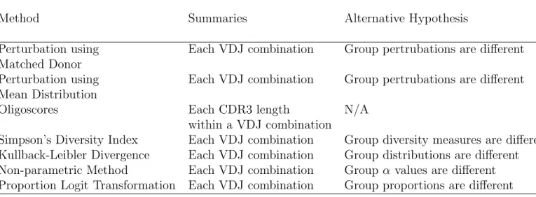
Table 1 shows a summary of the methods described and test that is being performed. Table 1: Table of Methods for Analyzing TCR Sequencing Data

Method Summaries Alternative Hypothesis

Perturbation using Matched Donor

Each VDJ combination Group pertrubations are different

Perturbation using Mean Distribution

Each VDJ combination Group pertrubations are different

Oligoscores Each CDR3 length

within a VDJ combination

N/A

Simpson’s Diversity Index Each VDJ combination Group diversity measures are different

Kullback-Leibler Divergence Each VDJ combination Group distributions are different

Non-parametric Method Each VDJ combination Group α values are different

(38)

1.6.8 Multiple Comparisons

Testing many independent hypotheses runs the danger of identifying significant differences that are the result of random chance. Methods such as the Bonferroni correction aim to control the probability of making a Type I error. This means that these methods also control the simultaneous correctness of all rejections [Benjamini and Hochberg, 2000]. However, the Bonferroni method is conservative and results in a substantial loss in power for individual tests. For high-throughput technologies it is more important to find all possible differences at the cost of getting a few hypotheses wrong.

The false discovery rate is defined as the expected ratio of erroneous rejections to the number of rejected hypotheses. Benjamini and Hochberg [1995] showed that this procedure

has a substantial increase in power over classic α controlling methods. The procedure was

shown to control the FDR at a lower level than desired so the adaptive procedure was created [Benjamini and Hochberg, 2000].

Letmrepresent the total hypotheses that we wish to test andm0 represent those that are

true. LetRdefine the total number of hypotheses rejected andV denote the number of those

hypotheses that were rejected incorrectly. Note that V is an unobservable variable. Using

these definitions the effective error rate is E[_mV

0] and the type I error rate is P(V ≥1). By

testing each hypothesis at level α we guarantee E[_mV

0]≤α but not P(V ≥1)≤α. Using a

procedure such as the Bonferroni by testing each hypothesis at _mα guaranteesP(V ≥1)≤α.

However, in the FDR procedure the error of falsely rejecting a null hypothesis is captured

by the random variable Q = V_R, the proportion of false-positives [Benjamini and Hochberg,

1995]. Thus, F DR=E(Q) =E V R .

Benjamini and Hochberg [2000] showed that when m0 < m the FDR is smaller than or

equal to the Type I error rate. Thus any procedure that controls the Type I error rate also

(39)

controls the FDR. But if you are only controlling the FDR then an improvement in power

is expected. The following procedure is shown to control the FDR at level q and improve

power:

1. Let P(1) ≤...≤P(i)≤...≤P(m) be the ordered p-values.

2. Let k be the largest i for which P(i) ≤ _mi q.

3. Reject all k ordered hypotheses.

The proof that this procedure controls the FDR is based on the lemma that says for

m1 =m−m0 false null hypotheses the test procedure satisfies the inequality [Benjamini and

Hochberg, 2000]

E(Q|Pm0+1 =p1, ...., pm =pm1)≤

m0 m q

Thus, when some of the null hypotheses are rejected the FDR is controlled at a level less

than q. So there is once again room to improve power in this procedure. If m0 was known

then E(V) = m0α and r(α) = v +s where s is the number of null hypotheses rejected

correctly. So the new estimate of the FDR can be [Benjamini and Hochberg, 2000]

ˆ Qe(α) = ˆ v(α) r(α) = ˆ m0α r(α).

Then to control the FDR at level q we can follow the following procedure

1. Let k be the largest i for which P(i) ≤ _m_ˆi₀q.

2. Reject all k ordered hypotheses.

The final problem is how to estimatem0. A graphical method can be used. If you consider

the p-values to be independent, under the null hypothesis they should follow a uniform[0,1]

(40)

origin and slope of S = 1

m+1. When there are false null hypotheses they tend to stack at the

lower end. However, the upper end should continue with a linear relationship. Thus, we can

use the slope of the higher p-values to solve form0. Benjamini and Hochberg [2000] suggest

the estimate of m0 to be calculated as follows.

1. Calculate slopes Si = _m1₊₁−p₋i_i and continue as long asSi ≥Si−1

2. Stop once Sj < Sj−1.

3. Then ˆm0 = min(_S1_j + 1, m).

1.7 Discussion

In this chapter we discussed T-cell biology and the ImmunoSEQ platform used to analyze the T-cell repertoire. Further, different methodologies were described to analyze the high-throughput sequencing data generated by the ImmunoSEQ assay. In the next chapter, we will apply these methodologies to a hematopoietic stem cell transplantation data set. In Chapter 3, we will discuss how high-throughput sequencing data can be considered compositional data and the analytical challenges that can present. Finally, the same HSCT data from chapter 2 will be analyzed as compositional data.

(41)

2 Applications to TCR sequencing data

2.1 Introduction

In this chapter, HSCT data (described in section 2.3) were analyzed using the methodologies described in chapter 1. To determine what pre-processing steps other researchers used, previously published data were reanalyzed. Finally, the differences in the methods were discussed.

2.2 Reanalysis of Published TCR data

We acquired the data from Dr. Harlan Robins’ lab that were analyzed in the 2012 paper titled “Ultra-sensitive detection of rare T-cell clones” [Robins et al., 2012]. This article describes the Adaptive Technologies ImmunoSEQ technology and it’s ability to detect T-cell clones. Thus, it was useful to reanalyze the data to determine the exact process used to perform the analysis. Specifically, we acquired replicate data for one patient but were unable to obtain the spike-in data used in the experiments. The data that we acquired included samples DNA A, DNA B, PCR A1, PCR A2, SeqA1b and SeqA1a.

We performed a similar analysis and compared our results to that reported by Robins et al. [2012]. In the publication, the authors were not specific about their data processing procedures so several different attempts were made to replicate their results. The first step required deciding whether to use all the sequences or a subset. The sequences are flagged by Adaptive Biotechnologies software as productive (usable proteins) or non-productive and through trial and error we discovered both productive and non-productive sequences were used for the analysis performed by Robins et al. [2012]. Next, in order to compare counts between replicates the files needed to be merged. The CDR3 sequences can be merged either by amino acid or nucleotide sequence and through trial and error we discovered Robins et al. [2012] merged by nucleotide sequence.

(42)

log-log plots are almost identical. Thus we established in our reanalysis the specific process the authors undertook. We noted a small difference between the total number of shared sequences between samples SeqA1a and SeqA1b. The authors identified 150,612 sequences but our analysis identified 150,567.

Figure 6: Reproducibility Plots The plots show frequencies of unique sequences from

different samples.

2.3 Data

Thirteen patients with hematological disorders who underwent HSCT were included in this study. This was a randomized phase II trial conducted at Virginia Commonwealth University

(43)

of a reduced intensity condition regimen for patients undergoing HSCT [Meier et al., 2013]. Human leukocyte antigen (HLA) matching was done and only patients with 7 of 8 or 8 of 8 matches were eligible for transplantation. HLA is a protein found on most cells in the body and there are 8 major types. The best transplant outcomes happen when patient and donor HLA’s are closely matched. Note that the TCR’s present are also determined by the protein they recognize along with the HLA’s present. Thus, the sample data could be skewed despite the close HLA matching. Peripheral blood stem cells were collected from the donor and recipient whole blood samples were collected post-HSCT. The goal of this analysis was to identify differences at the molecular level between T-cell repertoires of patients who suffered from GVHD and those that did not. Eight patients suffered from GVHD and five did not. T-cell sequencing data was generated using the ImmunoSEQ technology described in section 1.2. The methods described in section 1.6 were applied to the data and the results are described in the following sections.

All data analyses were performed using the R programming environment version 3.1.1 [R Core Team, 2014]. Only sequences that could result in usable proteins (productive sequences) were used in the analyses. Further, reads per million (RPM) were calculated for each sample and used in the analyses. RPM were calculated by dividing each CDR3 frequency by the total number of CDR3 sequences and multiplying by one million. VDJ combinations were filtered out to keep only combinations that had counts for at least 7 patients, leaving 947 VDJ combinations for analysis. CDR3 length summaries were obtained by summing all the CDR3 RPM’s of the same length within each VDJ combination. Further data management applied to a specific method will be described in the following sections.

2.4 Permutation Tests

Because of the low sample size (13 patients) permutation tests were used to compare groups. In this case, there are two samples that have been drawn from two distributions that may

(44)

independent of the GVHD group from a distribution, G. Thus, the null hypothesis to test is that the two distributions are equal and the alternative is that they are not equal. That is

H0 :F =G

Ha :F 6=G

Under the null hypothesis, any of the 13 observations could have come from either

distribu-tion F or G. All 13 observations were considered as a single set of values. A sample of size

five was drawn without replacement from this set of values to represent the no GVHD group. The remaining eight observations represent the GVHD group. 1000 random samples were

drawn in this manner. The absolute difference between group means, |µˆ∗|, was calculated

for each permutation. The p-value is then calculated as follows

p-value = #(|µˆ

∗_{| ≥ |}_µ_ˆ_|₎

1000 (39)

where |µˆ| is the absolute difference in means using the original sample. Thus, this is the

probability that the statistic was greater than that which was observed using the original sample [Efron and Tibshirani, 1994]. P-values were calculated for all 947 VDJ combinations considered for analysis. The p-values were then corrected for multiple comparisons using an

FDR threshold of 0.05. All permutation tests and FDR corrections were implemented in the

R programming environment.

2.5 CDR3 Distribution Perturbation Results

The CDR3 Distribution Perturbation method described in section 1.6.1 was adapted for

TCR sequencing data and applied to the study data. Each possible VDJ combination, f,

was examined individually. There were 947 perturbations calculated for each sample after filtering. The perturbations were calculated both as a perturbation from each donor’s T-cell

(45)

distribution,D_kdf , and as a perturbation from an average donor T-cell distribution,D_kaf . Df_kd

measures the perturbation from each donor and can be considered as a measure of how similar

the recipient is to the donor. D_kaf measures the perturbation from a control distribution and

can be considered to measure how different the samples are from each other. Depending on which calculation is used the interpretation of the difference between the GVHD and no GVHD groups is slightly different. Permutation tests described in section 2.4 were used to test for differences between the recipient GVHD and no GVHD groups.

The probability of each CDR3 length, i, was calculated using equation 8. The RPM were

summed for each unique CDR3 length and then divided by the total RPM present within

the VDJ combination of interest to calculate the CDR3 length probability, Ai. First, the

perturbation for each recipient was calculated as a perturbation from their matched donor. The donor CDR3 length probabilities were calculated in the manner described above. The perturbations were also calculated as a perturbation from a mean distribution of the 13 donors. The mean distribution was calculated by averaging the probability of each CDR3

length across all 13 donors. The perturbations were calculated using equation 10, wherek is

each sample and cis the control distribution. The control distribution is either an average

donor distribution or the matched donor distribution.

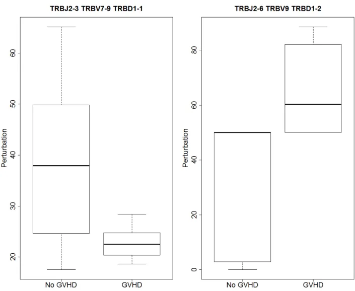
Then statistics were calculated using each matched donor for each VDJ combination and tested for differences between the GVHD and no GVHD groups. After adjusting for multiple comparisons using the Benjamini and Hochberg FDR method described in section 1.6.8, there

were two significant differences (FDR <0.001). The distribution of the statistic for the two

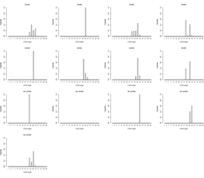
signifcantly different VDJ combinations can be seen in Figure 7. The figure shows boxplots where the median, 25th and 75th percentiles make up the box. The whiskers extend to 1.5 times the interquartile range (IQR) and if there are outliers they are represented by dots outside the whiskers. Table 2 shows the median perturbations and observed FDR for the two VDJ combinations. It was of interest to determine why the differences are in opposite directions. Looking at Figures 9 and 10 it appears as though the VDJ combination

(46)

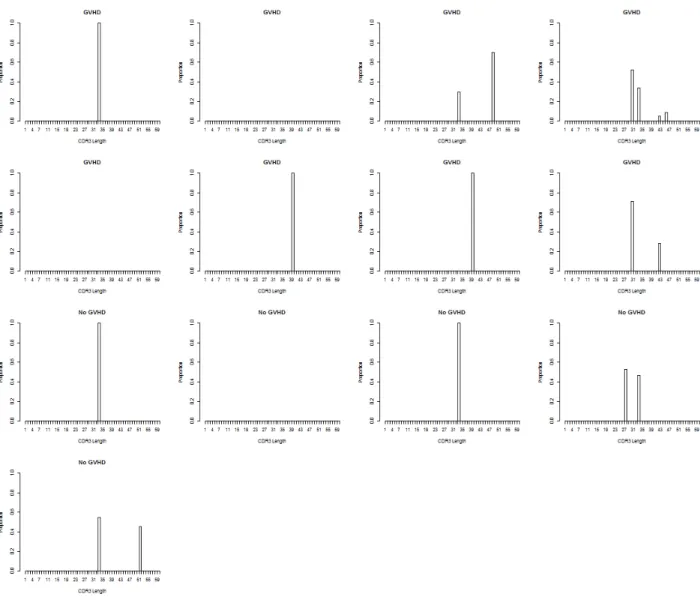
TRBJ2-6 TRBV9 TRBD1-2 is not present in a large number of the samples. Figure 9 shows the CDR3 length distributions in the donors for VDJ combination TRBJ2-6 TRBV9 TRBD1-2 and Figure 10 shows the CDR3 length distributions in the recipients for VDJ combination TRBJ2-6 TRBV9 TRBD1-2. Matched donors and recipients are in the same positions in the 2 figures. The low prevalence of this VDJ combination in the sample population could be causing the results of the test to be skewed.

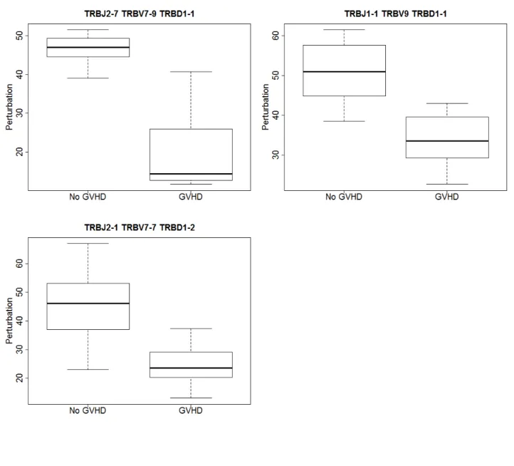
Second the statistics were calculated using a mean donor distribution as a control for each VDJ combination. After adjusting for multiple comparisons using the Benjamini and

Hochberg FDR method, there were three significant differences (FDR <0.001). The

distri-bution of the statistic for the three significantly different VDJ combinations can be seen in Figure 8. This is a measure of how different the No GVHD and GVHD groups are from each other. Table 3 shows the median perturbations and observed FDR for the three VDJ combinations. Note that the two analyses have no VDJ combinations in common.

(47)

Figure 7: Distribution of perturbation from matched donor statistic for the 2 significantly different VDJ combinations.

(48)

Figure 8: Distribution of perturbation from mean donor statistic for the 3 significantly different VDJ combinations.

Table 2: Median Perturbation Using Matched Donor Control

Median Median Observed

JGene VGene DGene No GVHD GVHD FDR<0.05

Perturbation Perturbation

TRBJ2-3 TRBV7-9 TRBD1-1 37.946 22.513 <0.001

TRBJ2-6 TRBV9 TRBD1-2 50.000 60.310 <0.001

(49)

Table 3: Median Perturbation Using Mean Control

Median Median Observed

JGene VGene DGene No GVHD GVHD FDR<0.05

Perturbation Perturbation

TRBJ2-7 TRBV7-9 TRBD1-1 47.001 14.364 <0.001

TRBJ1-1 TRBV9 TRBD1-1 51.051 33.529 <0.001

TRBJ2-1 TRBV7-7 TRBD1-2 46.154 23.571 <0.001

Figure 9: Distributions of CDR3 lengths from VDJ combination TRBJ2-6 TRBV9 TRBD1-2 donors.

(50)

Figure 10: Distributions of CDR3 lengths from VDJ combination TRBJ2-6 TRBV9 TRBD1-2 recipients.

High-Throughput Data Analysis: Application to Micronuclei Frequency and T-cell Receptor Sequencing

Virginia Commonwealth University

VCU Scholars Compass

High-Throughput Data Analysis: Application to

Micronuclei Frequency and T-cell Receptor

Sequencing

Mateusz Makowski

High-Throughput Data Analysis:

Application to Micronuclei Frequency

and T-cell Receptor Sequencing

Contents

List of Tables

List of Figures

1

T-Cell Receptors and the Adaptive Immune System

1.1

T-cell Biology

1.2

Technology for Measuring TCR

β

Clones

1.3

ImmunoSEQ Precision, Accuracy and Sensitivity

1.4

Unseen Species and Estimating the TCR

β

Repertoire using

ImmunoSEQ data

1.5

Application of TCR

β

Studies

1.6

Overview of Statistical Methods for CDR3 Data

1.7

Discussion

2

Applications to TCR sequencing data

2.1

Introduction

2.2

Reanalysis of Published TCR data

2.3

Data

2.4

Permutation Tests

2.5

CDR3 Distribution Perturbation Results