Model misspecification in the time series analysis

Davies, Neville (1977) Model misspecification in the time

series analysis. PhD thesis, University of Nottingham.

Access from the University of Nottingham repository: http://eprints.nottingham.ac.uk/13788/1/453158.pdf

Copyright and reuse:

The Nottingham ePrints service makes this work by researchers of the University of Nottingham available open access under the following conditions.

· Copyright and all moral rights to the version of the paper presented here belong to

the individual author(s) and/or other copyright owners.

· To the extent reasonable and practicable the material made available in Nottingham

ePrints has been checked for eligibility before being made available.

· Copies of full items can be used for personal research or study, educational, or

not-for-profit purposes without prior permission or charge provided that the authors, title and full bibliographic details are credited, a hyperlink and/or URL is given for the original metadata page and the content is not changed in any way.

· Quotations or similar reproductions must be sufficiently acknowledged.

Please see our full end user licence at:

http://eprints.nottingham.ac.uk/end_user_agreement.pdf

A note on versions:

The version presented here may differ from the published version or from the version of record. If you wish to cite this item you are advised to consult the publisher’s version. Please see the repository url above for details on accessing the published version and note that access may require a subscription.

MODEL MISSPECIFICATION

IN TIME SERIES· ANALYSIS

by

Neville Davies, B Sc, M Sc

Thesis submitted to the

University of Nottingham

for the degree of

Doctor of Philosophy

ACKNOWLEDGEMENTS

This research was carried out under the supervision of Dr Paul Newbold. I am extremely grateful for his stimulating guidance, encouragement and helpful criticism at every stage of the work.

I would also like to thank colleagues at the Department of Mathematical Sciences, Trent Polytechnic, for their support throughout; in particular I am most grateful to Mr M B Pate for consultations on many of the computer programs needed in the study. The computing facilities at Trent are also,

greatly appreciated.

Thanks and appreciation are also due to my wife who provided me with uncomplaining moral support during, what must have seemed to her, an unending project.

Finally, I should like to thank Mrs Jo Frampton for her meticulous care and patience in typing this thesis.

CONTENTS CHAPTER 1

I NTRODUCTI ON

1.1 Motivation

1.2 Notation: the Box-Jenkins approach to univariate model building

1.3 Notation: forecasting

1.4 Forecasting with misspecified models

1.5 Summary of chapters 2 - 6

CHAPTER 2

SOME SAMPLING PROPERTIES OF SERIAL CORRELATIONS AND THEIR CONSEQUENCES FOR TIME SERIES MODEL DIAGNOSTIC CHECKING

2.1 Introduction

2.2 Sample moments of the autocorrelations of white noise

2.3 Levels of significance of the portmanteau test statistic

2.4 Sample moments of the autocorrelations of moving average processes

2.5 Conclusions

CHAPTER 3

FORECASTING FROM MISSPECIFIED TIME SERIES MODELS WHEN THE DEGREE OF DIFFERENCING IS CORRECTLY ASSUMED

3.1 Introduction

3.2 Fitting autoregressive models to any time series of the ARMA type

3.3 Fitting mixed autoregressive moving average models to any time series of the ARMA(p,q) type

3.4 Comparison of forecasts for correct and misspecified models with the coefficients in each being given

3.5 Fitting autoregressives when we allow the parameters to be determined by the autocorrelations of the true process 3.6 A property of P(h) for fitting autoregressive models to

ARMA(p,q) processes 1 3 10 13 15 17 20 26 37 52 53 54 60 63 72 77

3.7 Percentage loss for fitting AR(p) models to ARMA(p,q) processes

3.8 Percentage loss for fitting AR(p) models to ARMA(p,q)

processes taking estimation error into account in the fitted model

3.9 Percentage loss for fitting any ARIMA(p',d

,en

model to any other ARIMA(p,d,q) process; d ｾ 1

3.10 Percentage loss for fitting ARIMA(p,d,O) models to ARlMA (p,d,q) processes

3.11 Percentage loss for fitting ARIMA(p',d ,0) to ARIMA(p ,d,q) processes taking estimation error into account in the fitted model

3.12 Conclusions CHAPTER 4

SOME POWER STUDIES OF THE BOX-PIERCE AND BOX-LJUNG PORTMANTEAU STATISTICS

4.1 Introduction

4.2 The distribution of residual autocorrelations from fitting an AR(p) model to any ARMA(p,q) process

,

4.3 The portmanteau statistics Sand S for fitting AR(p) models

82 90 99 104 III 113 128 129 to ARMA(p,q) processes 140

4.4 Simulation results for the power of the portmanteau statistics

4.5 Conclusions

CHAPTER 5

FORECASTING FROM MISSPECIFIED TIME SERIES MODELS WHEN THE ASSUMED DEGREE OF DIFFERENCING IS TOO LOW

151 163

5.1 Introduction 165

5.2 The mean and variance of the sample autocorrelations for an

IMA(l,l) process 168

5.3 The mean and variance of the sample autocorrelations for

any ARIMA(p,l,q) process 178

5.4 Asymptotic forecast error variances and percentage losses

5.5 Conclusions 190

CHAPTER 6

MODEL MISSPECIFICATION IN TIME SERIES ANALYSIS: RETROSPECT AND PROSPECT

6.1 The results of model misspecification so far covered 191

6.2 Unsolved problems in this study 196

6.3 Further problems in misspecifying time series models 198

6.4 Time series error misspecification and spurious regressions 203

6.5 Conclusions 218

ABSTRACT

The Box and Jenkins (1970) methodology of time series model building using an iterative cycle of identification, estimation and diagnostic checking to produce a forecasting mechanism is, by now, well known and widely applied. This thesis is mainly concerned with aspects of the diagnostic checking and forecasting part of their methodology.

For diagnostic checking a study is made of the overall or 'portmanteau' statistics suggested by Box and Pierce (1970) and Ljung and Box (1976) with regard to their ability for detecting misspecified models; analytic results are complemented by simulation power studies when the fitted model is known to be misspecified. For forecasting, a general approach is proposed for determining. the asymptotic forecasting loss when using any fitted model in the class of structures proposed by Box and Jenkins, when the true process follows any other in that same class. specialisation is made by conducting a thorough study of the asymptotic loss incurred when pure autoregressive models are fitted and used to forecast any other process.

In finite samples the Box-Pierce statistic has its mean well below that predicted by asymptotic theory (so that true significance levels will be below that assumed) whilst the Box-Ljung statistic has its mean approximately correct. However, both statistics are shown to be rather weak at detecting misspecified models, with only a few exceptions. Asymptotic forecasting

loss is likely to be high when using even high order autoregressive models to predict certain simple processes. This is especially the case when allowance is made for estimation error in the fitted models.

Finally, some outstanding problems are outlined. One of these, namely the problem of misspecified error structures in time series regression analysis, is examined in detail.

1.1 Motivation

CHAPTER 1

INTRODUCTION

This research was initially motivated by an apparent need to question whether or not a model that had been fitted to a time series was the correct one, and to examine the consequences if the fitted model was misspecified.

Over recent years many sophisticated techniques have been developed to produce superior models that will provide a better fit to the data at hand and (hopefully), therefore, produce a better forecasting mechanism for future, as yet unrealised, values from the same series. In essence, these techniques generally assume, a priori, the model to be fitted (or base model choice on the evidence of the data) and so if a misspecification of the model occurs, for some reason, it would seem reasonable to conjecture that the consequences could be serious from a forecasting point of view. (Moreover, some of these techniques are relatively expensive to use and

implement and so one could also ask whether a less sophisticated and expensive method might not do almost as well from a forecasting point of view. These ideas and problems are really concerned with the philosophy and need for

forecasting via the fitted model and have been raised in the literature before. See, for instance, Granger and Newbold (1975) and Chatfield and Prothero

(l973b)).

We shall, in this study, restrict ourselves to models within the general class of autoregressive integrated moving average (ARIMA) processes, which have been studied thoroughly by Box and Jenkins (1970), and ask the general question whether particular fitted models in this class can forecast as well as the optimum forecast function for the process, which is also assumed to follow from a model in the same class. For certain models in this class, the Box and Jenkins procedure can be expensive in time and money for

adequate analysis and also in the expertise needed to apply the techniques (see, for example the conclusion in Chatfield and Prothero (1973a, p 313».

In one sense, then, we shall adopt the attitude of "doing all the wrong things", which on the face of it seems certainly sub-optimal, but is

eminently more sensible if one views the whole model building procedure after the event and asks whether or not the "true" model for the data has been produced by the techniques employed. Of course, these techniques usually have built-in checks to test whether the model produced can be considered to be the 'correct' one. By their very nature. model checking tests cannot

entertain all possible alternative models that could have been fitted, so that they will naturally not be equally powerful against all alternatives. One of the objectives, therefore, will be to try to isolate some of the model misspecifications which are more serious and which could be ignored (for some reason or another) by some of the diagnostic checks on model adequacy.

Furthermore, some authors in the recent past (Chatfield and Prothero (1973a),Prothero and Wallis (1976» who have fitted Box-Jenkins type models have doubted the ability of the so called portmanteau statistic (Box and Pierce (1970» to detect model misspecification. The need to analyse in detail this doubt about this particular diagnostic check was another motivation for examining model misspecification.

Chatfield (1977) does not believe there is a "true" model, but rather that a fitted model can provide a simple and useful approximation to some far more complicated truth. This view seems entirely reasonable. However, in this study an underlying assumption will be that there does exist some relatively simple true model. We will then examine the consequences which follow when the analyst fails to correctly specify this model. Such an approach seems well worthwhile, and moreover it would seem reasonable to argue that the results derived would continue to be useful in a more general context which would allow for Chatfield's objection. This more general view would be that although reality is typically exceptionally complicated, it is nevertheless the case that a particular simple model will generally provide a sufficiently good approximation to that reality for practical purposes (for example, forecasting). This simple model could then, in practice, be

regarded as "truth", and the consequences of operating with other simple models could safely be examined as if this original simple model were indeed a "true model". After all, since model selection is generally based on sample evidence, it is reasonable to expect that the analyst will on occasions fail to find the appropriate simple model. Furthermore, in those situations in which an underlying model is assumed a priori, it may often be the case that the assumed model differs appreciably from the particular simple model which is appropriate.

One of the more recent developments in time series analysis has been the practical applications of multivariate time series techniques as a natural extension of the univariate work of Box and Jenkins (1970). In a recent paper Haugh and Box (1977) fit a multivariate Box-Jenkins model and suggest that the possibilities of making errors in the first stage of the multivariate procedure, namely fitting univariate models in the ARIMA class to each series under consideration, deserves further research. This thesis attempts to show the results of univariate misspecifications in this class of models.

Another area which has aroused interest lately is the possibility of misspecifying the residual structure in a time series regression analysis (Granger and Newbold (1974), Pierce (1977», and the former paper provided the stimulus for examining residual error misspeci fication.

1.2 Notation: the Box-Jenkins approach to univariate model building

We summarise here the general approach to univariate model building as advocated by Box and Jenkins (1970) as an introduction to the general

notation used throughout this study. If appropriate in later chapters, the notation may be restated for clarity of exposition. More detailed reviews of the Box-Jenkins approach are given by Nelson (1973), Newbold (1975), Chatfield

(1975) and Granger and Newbold (1977). Specific examples may be found in papers which include Chatfield and Prothero (1973a),Bhattacharyya (1974), Brubacher and Wilson (1976) and Saboia (1977). A summary of many Box-Jenkins analyses may also be found in Reid (1969) and Newbold and Granger (1974).

For a review of the current state of time series analysis in general see Chatfield (1977) or Newbold (1978).

Denote by (X

t ), or simply Xt , a discrete time series at equally spaced instants of time. Available for study is a sample of n observations of X

t , X ,X , ••• ,X and we shall assume the prime objective is to forecast 1 : 3 n future values Xn+h (h ｾ _{1). The series Xt is said to follow an ARIMA(p,d,q)}

process if

where B is the backshift operator such that BX t -X t -J ., and

.0(B)

Q(B)

=

1 -

P.

B -

.0

B:3 -1 :3

=

1 + 9 B + 9 B:3 + 1 :3

...

(1.1 ) X t -1 ,and by repeated

with p, d and q non-negative integers. Here at is a process with zero mean, fixed variance 0a2, and with corr{at,a

s)

=

0 , t I s . Such processes are called "white noise". The roots of the polynomial equations in B,

.0(B)

=

0

and 9(B) = 0 will be required to lie outside the unit circle IBI = 1 to ensure stationarity and invertibility conditions (see Box and Jenkins (1970) pp 73-74). The constants

p.

,.0 , •••

,p

are said to be the autoregressive (AR)

1 2 P

parameters whilst 9 ,9 , ••• ,9 are termed the moving average (MA) parameters.

1 : 3 q

A pure AR process has d

=

0 and q

=

0, whilst a pure MA process has d

=

0

and p

=

O. The integer d indicates the order of differencing required to reduce the process to stationarity. If d

=

0, with

pI

0 and q

I

0 the structure (1.1) is said to be an ARMA(p,q) process.

The Box-Jenkins methodology for constructing ARIMA(p,d,q) models is based on a three step iterative cycle of (i) model identification (ii) model

estimation (iii) diagnostic checking on model adequacy. After this cycle has been successfully completed the model fitted is then ready to be used in a rather important way, namely to forecast future observations of the series giving rise to structure (1.1).

(l)The notation used here differs slightly from that of Box and Jenkins (1970), who use 9(B)

=

1 - 9

1B - ••• - 9qB q

, but is in line with that of Granger and Newbold (1977).

We briefly describe here the ideas behind (i) and (ii) but the main theme in this thesis is to examine the consequences of misspecifying (1.1) by looking in detail at one technique commonly employed in the stage (iii) of diagnostic checking and the comparative quality of forecasts obtained from the misspecified model.

(i) Identification

At the identification stage one selects values of p,d,q in the model (1.1) and obtains initial, rough estimates of

p.

,p , ..•

,p, ,

9 ,9 , ••• ,9 using

1 2 P 1 2 q

procedures which are in general, inexact, and require a good deal of judgement. The two main tools for doing this are the autocorrelation function and partial autocorrelation function.

Let Yk

=

｣ ｯ ｶ ｛ ｾ Ｌ ｘ ｴ Ｋ ｫ ｝ ［ then the autocorrelation at lag k is

(1.2)

where y will be the variance of the process. The partial autocorrelation at

o

lag k, usually denoted ｾ ｫ ｫ Ｇ is the partial correlation between X

t and Xt_k'

given X

t -J . (j = l, •••

,k - 1),

and may be derived by solving the set of

equations

k

Pj =

ｩ

ｾ

ｬ

ｾ

ｫ ｩ

_{Pj - i} (j = 1, ••• ,k) ( 1.3)

Using the given set of data X ,X , ••• ,X ,

Y

k is estimated by ck' where 1 2 n n-k C_{k :}

ｾ

J:

1 (Xt - X)(Xt+k - X) (1.4) n

and

X

= ｾ Xt/n. The sample autocorrelation

(1.5)

is then used to estimate P

k• (Note that, in general (1.4) is defined with a mean subtracted off. We shall, in later chapters, use (1.4) and (1.5) without

a sample mean subtracted when it is clear the true mean of the process is zeroJ Thus, the estimates of

P

kk are obtained by substituting rk for Pk in (1.3). Based on the characteristic behaviour of the autocorrelation and

partial autocorrelation functions of different members of the class of stochastic models (1.1) (as summarized, for example by Box and Jenkins Ｈ Ｑ Ｙ Ｗ Ｐ ｾ

p 79 or Granger and Newbold (1977), p 74) and using the sample estimates, a tentative identification of the orders p,d and q can be made.

Clearly the extent to which one can reasonably hope for success in model identification depends on the degree of similarity in the behaviour of the parent and sample autocorrelation and partial autocorrelation functions. All other things being equal, the longer the data set, the better the chances of success. It is generally held that for samples of less than about 45-50 observations, sampling variability is likely to render all but the simplest members of the ARIMA class virtually impossible to detect. Moreover, even with samples of 50-100 observations, commonly found in Box-Jenkins analyses, it seems reasonable to expect that misspecification, of the kind to be studied in this thesis, will occur fairly frequently.

(ii) Estimation

Once the orders p,d,q have been identified, the next stage in the cycle is to efficiently estimate the tentatively identified parameters to produce

/ \ " I' It II ,.

estimates

p.

Ｌ ｾ

, •••

Ｌ ｾ

,

Q ,Q , ••• ,Q • A least squares minimisation procedure

1 2 P 1 2 q

is usually employed on the conditional expectations of the residuals. It can be shown that the least squares procedure, for moderately large sample sizes, produces estimates which are very nearly maximum likelihood. (See Box and Jenkins (1970), Chapter 7 or Newbold (1974) for details.) The main problem with the procedUre is that since the function that has to be minimised is not a simple function of the parameters to be estimated, the numerical minimisation can be rather expensive in computer time. other problems such as obtaining the starting up values for the procedure may be solved by methods given by

Granger and Newbold (1977), p 88. (iii) Diagnostic checking

Box and Jenkins (1970) recommend several post-estimation checks that may be employed to attempt to detect a misspecification in the class (1.1). They do emphasise that individually the tests have certain disadvantages, implying perhaps that each should not be used in isolation. However, one of these,

to be described shortly, has been used extensively in the literature apparently as the only diagnostic check to be tried on fitted models. One of the main objectives in this thesis will be to attempt to show this particular test in isolation is rather inadequate at detecting a mis-specification in the class (1.1).

The method of overfitting is concerned with adding in extra coefficients in the estimated ARMA(p,q) model for the differenced series, so that a new ARMA(p+p*,q+q*) model could be estimated in the manner indicated above. If the original ARMA(p,q) model is adequate for the differenced data, the estimation procedure should reject the extra coefficients ｾ +" (j = l, ••• ,p*)

p J

and Q " (j

=

l, ••• ,q*), so that their estimates differ insignificantly from q+J

zero. However, Granger and Newbold (1977) recommend fitting two different models namely ARMA(p + p*,q) and ARMA(p,q + q*) as alternatives since they

show in their section 3.4, p 80, that the addition of extra coefficients to both sides of a correct model can lead to indeterminacy. This will cause the point estimates of the coefficients to be meaningless and their estimated

standard deviations to be very large.

If the fitted model is of the form (1.1) and it is the true model, the residuals

constitute a white noise process. Anderson (1942) has shown that the sample autocorrelations of the residuals a ,a , ••• ,a , given by

1 2 n

n n

r k

=

.Jk+1 atat-k/.Jl at 2

are, for moderately large samples, uncorrelated and normally distributed with standard deviations n-

t .

Thus we see that knowledge of the at and hence the r

k would provide us with information on the process. However, the fitted model (1.1) has to be estimated, as indicated in (ii) above so that the residuals become

with the sample autocorrelations now given by

A Box and Pierce (1970) derived the asymptotic distribution of the r

k and showed that the standard deviations can be much less than n-

t

for small values of k. Some thoughlon this latter point shows that it comes as a result of actually fitting the time series model; the parameters in the model are so estimated that the residuals for the fitted structure are as much like white noise as possible. Hence the first few autocorrelations of

the residuals will be close to zero.

To make this point rather more concretely, suppose we attempt to fit a pure AR(l) model to white noise. From Box and Jenkins (1970), p 278 an asymptotically efficient estimate of the autoregressive parameter will be the first sample autocorrelation of the process X_t

=

at. Hence this will be given by r above.

1

It follows that the residuals from the fitted model will be

x -

_t r X

1 t - l

whereas the true model that fits this data is the AR(l) process

in which

p.

=

o.

1

(1. 6)

(1. 7)

Hence r is effectively being used to estimate

p.

=

O. Simulation

1 1

stUdies were conducted in which samples size 50 were generated from a white noise series and (1.7) was estimated over 1000 simulations, calculating the

...

mean and variance of the residual autocorrelations r

k for (1.6). This was repeated for a further 1000 series for 'residuals' created by (1;7) in which

¢.

=

O. We note that in connection with (1.7) we are assuming we know the

1

correct parameter value whereas in (1.6) we are not. Results of the two simulation studies are given in Table 1.1.

Mean rA for k Mean r"-_k for 50.var[r k

J

50.var[rk

J

TABLE 1.1

EMPIRICAL MEAN AND VARIANCE OF THE SAMPLE RESIDUAL

AUTOCORRELATIONS OF (1.6) AND (1.7) k 1 2 3 4 (1.6) -0.001 -0.017 0.003 0.004 (1.7) 0.000 0.002 0.003 0.006 for (1. 6) 0.036 0.930 0.881 0.919 for (1. 7) 0.954 0.961 0.922 0.958 5 6 0.000 -0.001 0.000 0.000 0.891 0.809 0.916 0.825

We see that the empirical means agree reasonably and so do the values of n ｶ ｡ ｲ ｛ ｾ ｫ ｊ for k ｾ 2. But at k

=

1 we can conclude that the fitting procedure has caused the variance of the first residual autocorrelation to be greatly deflated. This deflation was noted initially by Durbin (1970).

It therefore seems that for the general fitted model of the form (1.1) a comparison of

ｾ

ｫ

with

±

2n-

t

will be unreliable for low values of k, but should provide a general indication of possible departure from white noise in the residuals, provided it is remembered the bounds will tend to under-estimate the significance of any discrepancies.

The Box-Pierce portmanteau statistic

Box and Pierce (1970) showed that the statistic

is asymptotically distributed as X2 with (m - p - q) degrees of freedom, (where m is usually about 20 for reasons given in Chapter 2) and its use in model diagnostic checking has been advocated by Box and Jenkins (1970), p 291. The hypothesis of adequate model specification would be rejected if the

autocorrelations of the residuals overall departed significantly from white noise, so that a high value of S could be taken as an indication of model misspecification. As notedin section (1.1) many authors have doubted the

ability of S to detect model misspecification and Chapters 2 and 4 concentrate

on the problem of applications of S when the model is correctly and incorrectly specified respectively. We merely note here that in the simulation studies reported above the empirical mean value of S over the 1000 simulations, with m

=

20, was for the fitted model (1.6), 13.94.

Clearly, this value is rather a long way from the asymptotic mean of 20 - 1

=

19 and so we would not expect the use of S in the above situation to be able to detect any misspecification if we were fitting an AR(l) model. The sample size n

=

50 is certainly considered 'moderate' in practical time series analysis and so a closer look (at least) at the exact mean of S, as defined above, is certainly warranted.

Wilson (1973) has defended the above statistic by claiming it cannot be expected to detect model inadequacies outside the class of models (1.1) for which it is designed; we shall show in Chapters 2 and 4 that it is weak even at detecting misspecifications within the class (1.1).

1.3 Notation: Forecasting

We summarise here some of the main results in the theory of optimal linear forecasting techniques, following closely the notation of Granger and Newbold (1977). Also given is a brief review of Box-Jenkins forecasting methods

together with some comments on the well known exponential smoothing techniques for forecasting. (For a Bayesian approach in forecasting see Harrison & Stevens Ｈ Ｑ Ｙ Ｗ Ｖ ｾ Ｉ

Let X

t be a zero mean stationary invertible ARMA(p,q) process

which may be written

=

at + d ₁ at _-1 + d _{2 - 2} at + .•••

By seeking a linear forecast of X h (h ｾ 1) in the form

n+

co

f _n, h

=

_J=O .E w. _J, h X _n-J .

(1.8)

and using a least squares criterion, Granger and Newbold (1977), p 121, show that the optimum forecast is of the form

<Xl

f _n, h = _{J=O J+ n-J} .E d. ha . d = 1

o

Let e h be the h step forecast error X h - f h; then if V(h)

n, n+ n,

(1. 9)

denotes the variance of this error (equivalently sometimes known as the asymptotic mean square error), Granger & Newbold show that e h is an

n, MA(h - 1) process with

h-1

V(h) _{= ｊ}Ｎ_ｾｾ _ｏ d.2 2 _{J O"a} (1.10)

and that forecast errors from the same base, n, are typically correlated with (for k ｾ 0)

h-1

E[en,h en,h+k

J

=

ｪ

ｾ

ｏ

､ ｪ ､ ｪ

Ｋ

ｫ

ｏ

Ｂ

｡

Ｒ

(loll)

Also from the MA(h - 1) process that the h step forecast errors follow one may obtain the updating formula

f = f + d (X - f )

n ,h n-1 ,h+1 h n n-1 ,1 ( 1.12)

which can be very useful in generating the new optimal h step forecasts given the forecasts up to time (n - 1) and the most recent observed value in the series, X • This can save a considerable amount of computational

n

work in the calculation of new forecasts.

If, for example X_t is a pure MA(q) process

the theory leading to (1.9) gives (with Q = 1) o

f _n,h

=

This may be expressed in the form q-h

f h = .E Q. h(X . - f . )

n, J=O J+ n-J n-J-1,1

h>q

(1.13)

and can be used to generate forecasts given the infinite past. Starting up values will be a problem in practice although this will be mentioned later.

A useful formula can be derived for the sequence of optimal forecasts for given n and increasing h. It is easy to see that the coefficients on the

right hand side of (1.8) satisfy the following recurrence relation with the ARMA coefficients

I.

,p , ...

,1. ,

Q ,9 , ••• ,9 •

1 2 P 1 2 q

P d

k - J=l J

.E

p.dk -J .

=

Qk d. J = 0 (j < 0), k = 0,1, •• (1.14)

Thus, from (1.9) we can show that p f _n, h - _{J=l J} .1:

p.

f _n, h . _-J = where f .

=

Xn+' for j s;

o.

n,J J <XI .,l;: Q. ha . 1-0 1+ n-1 0, i > q

The sequence of forecasts may be obtained by replacing a . by

n-1

x . -

f . in (1.15).

n-1 n-1-1 ,1

(1.15 )

The above theory has assumed the process to be forecast is stationary; section 3.9, Chapter 3 generalises the previous methods to obtaining the

variance of the h step forecast error when the process followed is ARlMA(p,d,q). (See equation (3.88).) A forecast function similar to (1.9) and updating

formula similar to (1.12) may be derived easily although we do not need them here.

This section, so far has been concerned with univariate forecasting theory in a particular class of time series models. The fitting of a member of this class of models involving the identification, estimation and

diagnostic checking outlined in section 1.2 together with the above indicated forecasting functions, has become known as the Box-Jenkins forecasting

procedure.

For practical illustrations of forecasting using this procedure a very clear exposition is given in Granger and Newbold (1977), section 5.2, p 149.

As has been pointed out by many authors, this particular class of models is particularly flexible in its possible application to many commonly

occurring time series. These techniques tend to be a little complex to apply in practice and for that reason other, less sophisticated methods are

employed sometimes, though they are not typically optimal. The most commonly used of these is the exponential smoothing procedures which have the

Of course, with these techniques one generally sacrifices forecasting accuracy for simplicity of models, as the latter can be shown to be a very restrictive set of processes. (See, for example Harrison (1967).) In any case most of the exponential smoothing models can be shown to be special cases of a technique called Kalman filtering Ｈ ｋ ｡ ｬ ｭ ｡ ｮ Ｈ Ｑ Ｙ Ｖ ｡ ｾ Ｌ Ｑ Ｙ Ｖ Ｓ ｾ which has been known to engineers for some time.

Exponential smoothing methods have been proposed and developed by Holt (1957), Winters (1960), Brown (1962), Theil and Wage (1964), Nerlove and Wage (1964), Trigg (1964), Harrison (1965, 1967), Trigg and Leach (1967), Harrison and Stevens (1971), Cogger (1974). For a summary of the methods and comparison of these techniques from a forecasting point of view with Box-Jenkins methods see respectively Granger and Newbold (1977), pp 163-179 and

,

Newbold and Granger (1974).

Some of the results presented in this thesis may, at least indirectly, be of relevance to exponential smoothing since the great majority of these procedures assume a priori an underlying model. It will therefore

frequently be the case that to some degree or other the models assumed will be misspecified.

Our main concern in this thesis will be to assess the consequences for forecasting of misspecified models within the ARIMA(p,d,q) class.

1.4 Forecasting with missspecified models

One could regard all fitted models in time series analysis as misspecified since they will be estimated from sample data and one could never be sure

whether the fitted model is the 'last word' at describing the structure from which the sample was derived. Surprisingly little seems to have been done in the region of the consequences of misspecification of time series models in practice. Box and Jenkins (1970) p 298 indicate how the residuals may be used to modify a misspecified model; their diagnostic checks suggested in Chapter 8 should, in theory detect a misspecification so that a new cycle of

identification, estimation and diagnostic checking could be started, although these checks themselves depend in one sense on knowing the correct model.

Bloomfield (1972) has applied spectral techniques to the problems of

misspecification in autoregressive series, while Granger and Newbold (1977) derive the asymptotic mean square error for prediction using a misspecified model. Yamamoto (1976 a,b) derives the asymptotic mean square error of prediction in the class of ARMA(p,q) models taking estimation error into account in the fitted coefficients, but his methods assume the model is correctly specified. It would seem an investigation which combines and

extends the above methods of Granger

&

Newbold (1977) and Yamamoto (1976 a,b) by looking at misspecified models within the ARIMA(p,d,q) class would yield fruitful and interesting results.

Initial evidence for this is provided by McClave (1973) who conducted an empirical study of pure autoregressive approximations to first order moving average processes. His motivation for doing this was given by Durbin (1959) who used high order AR approximations to derive efficient estimates for moving average coefficients. McClave concluded that a significant bias was present in estimating the fitted AR coefficients, which would certainly have adverse implications for Durbin's procedure and for autoregressive spectral estimation techniques such as proposed by Parzen(1969).

In fact in this study we concentrate on fitting pure autoregressives when another model in the ARIMA(p,d,q) class is appropriate. (We could be accused at this stage of being guilty of 'assuming' the appropriate structure, a practice we have already stated in this chapter is a cause for concern; the best we could do would be to take the estimation of the 'correct' model into account, which although we do not do explicitly in this study, for reasons given in Chapter 3,we can expect our results to be little altered by this extra complication.)

The attraction of examining pure autoregressive fits stems from many areas. Firstly, provided the roots of the moving average polynomial 9(B) in

(1.1) lie outside the unit circle the process X_t can always be expressed as an infinite autoregressive process. This fact has led Kendall (1971) in his review of Box and Jenkins (1970) to conclude that we might as well be content\ with autoregressive series and let the order of the fitted AR model be high

enough to ensure independence of the residuals. Box and Jenkins (1973) disagreed, arguing their case for a parsimonious model for the time series, pointing out that problems might arise with a large number of parameters to be estimated. Of course, pure AR processes are very simply fitted and

estimated by least squares (see Box and Jenkins (1970), p 277) whereas mixed models in the ARIMA(p,d,q) class cause problems in estimation as we have already seen. The implication of Kendall's comments are that one will do progressively better by increasing the order of AR fit. This is certainly true if one considers fitting only, but we shall show in Chapter 3 that when one takes estimation error of the AR parameters into account one ｾ do

progressively ｾ by estimating more coefficients.

Along the same lines as the notation in section (1.3), we suppose our fitted model is within the ARlMA(p,d,q) class, say ａ ｒ ｉ ｍ ａ Ｈ ｰ ｾ ､ Ｚ ｱ Ｉ in the form

,

I(B)(l - B)dXt

=

@(B)rt (1.16)

where ｾ ｴ is now not necessarily white noise. The model (1.16) is developed fully in terms of obtaining forecasts, gn,h (say) and our basis of comparison is between f h from the correct model (1.1) and g h from the misspecified

n, n,

model. Specialisation to the case @(B)

=

1 takes place when we examine pure autoregressives.

1.5 Summaries of Chapters 2-6

Chapter 2 examines in detail the Box-Pierce statistic as advocated by Box and Jenkins (1970); in particular exact expressions are derived for the mean and variance of the statistic under the null hypothesis of adequate specification for the fitted ARMA(p,q) model. Using a central aXv2 approxima-tion theoretical significance levels are derived for fitting AR(I) models to AR(l) processes and these are compared with simulation studies. Some of the deficiencies of the Box Pierce statistic are overcome by a modification of the statistic and this is also examined in detail. Finally low order moments of the sample autocorrelations of moving average processes are derived for use in a later chapter.

Chapter 3 studies the asymptotic loss from a forecasting point of view of fitting a misspecified model in the ARlMA class to any other model in the same class when the order of differencing is correctly specified and looks in detail at the case of fitting autoregressives both with and without estimation error in the fitted coefficients.

Chapter 4 uses some of the misspecified models in Chapter 3 to examine the performance of the Box-Pierce statistic, and its modification, in

detecting the given misspecification. The asymptotic distribution of the residuals from a misspecified AR model are derived together with the asymptotic mean and variance of the Box-Pierce statistic under this mis-specified model. Empirical power studies are conducted on the ability of the two diagnostic statistics to detect misspecified autoregressive models when the true process follows particular models in the ARMA(p,q) class.

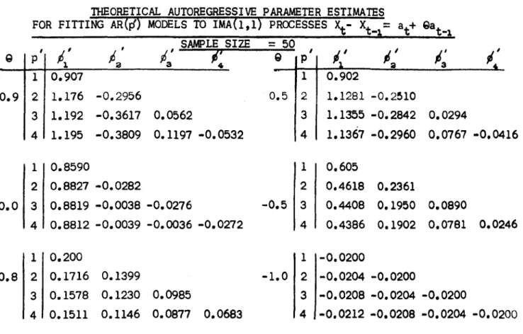
Chapter 5 considers the problem of underdifferencing a process in the ARIMA (p,d,q) class and examines in detail the case- of fitting AR models to the

lMA(l,l) process X_t - X_t

-1

=

at + 9at_1 • Expressions for the mean and variance

for the sample autocorrelations of the latter process are derived and used in the context of fitting the AR models. Finally, an approximate expression is derived for the asymptotic percentage loss of forecasting for this mis-specification, the result being verified by simulation studies.

Chapter 6 summarises the findings of Chapters 2-5 and suggests further areas of research in model misspecification. One of these areas, namely mis-specified error structures in regression analyses is looked at in the case of the error process being IMA(l,l) when the Durbin-Watson d statistic {Durbin and Watson Ｈ ｬ Ｙ Ｕ Ｐ ｾ Ｌ which is optimal for an AR(l) error structure, is used in an attempt to detect autocorrelation in these residuals and analysis proceeds under the (false) assumption that an AR(l) error structure is appropriate. Extensive simulation studies are reported.

CHAPTER 2

SOME SAMPLING PROPERTIES OF SERIAL CORRELATIONS AND THEIR CONSEQUENCES FOR TIME SERIES MODEL DIAGNOSTIC CHECKING

Summary

This chapter studies the sampling properties of serial correlations of white noise and, using these, explains why surprisingly low values of the Box-Pierce portmanteau statistic for testing model inadequacy (which have been reported in the literature recently), are very often obtained even when it is known a given model is inadequate. The main reason is that. even for moderately large sample sizes, the true significance levels are much lower than those predicted by the asymptotic theory on which the test is based. Approximations to the low order moments of the sample

auto-correlations of moving average processes are also derived for finite sample sizes in terms of the derived moments of the serial correlations for white noise.

2.1

Introduction

Suppose that a time series [X

t } follows a stationary ARMA (p,q) model ¢(B)X

t

=

Q(B)at

(2.1)

where BXt

=

\-1' ¢(B)

=

1 - ¢1 B - •••• - ¢pBP, 9(B)

=

1 + _{91 B} + ••• + _9qBq, [at} is a sequence of zero mean white noise which is assumed independent ｎ Ｈ ｏ Ｌ ｾ Ｉ Ｎ X

t in general could be the dth difference of an observed time series. In fitting to data ARMA(p,q) models of the type

(2.1)

an integral part of the methodology of Box

&

Jenkins (1970) involves diagnostic checks based on the residuals

(2.2) where the least squares estimates of the coefficients

$ ,$ , ... ,$

Ｌ ｾ Ｂ Ｂ ｾ ｱ

1 <3 P 1

are based on the observed series X ,X ""'Xn' 1 2

The auto correlations

k

=

1,2, ••• (2.3)

are calculated as a basis for the model checking. Box & Pierce

(1970)

studied their joint distribution. They initially examined the AR(p) model

and showed that approximately for moderately large nand m

r

=

(I - Q)r

...

...,

(2.4)

,,, ("

"

) where r = r , ••• ,r - 1 m , ..., r'= (r ,r , •• ,r) 1 2 m with n ｾ ata t_k t=k+t r k = n k = 1,2, .•• ,m

(2.5)

J1 a t :a and Q

=

X(X'X)-l X' with X= 1 0

'1

1

_(2.6)

'a '1 'm-1 'm-a 'm-p where (1 + • B + ••• )(1 - ｾ B

1 1

...

- ｾ p BP)

=

1. The approximation depends

upon m being moderately large, so that

'j

is negligible for j > m - p. Asymptotically the r

k are distributed as independent N(O,l/n) (see Anderson

(1942),

Anderson and Walker

(1964)

or Bartlett

(1946»)

from which it follows, since the matrix (I - Q) is idempotent of rank (m - p)

that the portmanteau statistic

(2.7)

is asymptotically distributed as X2 with (m - p) degrees of freedom. To deal with mixed processes of the form (2.1), Box and Pierce note that for moderately large n, the residual autocorrelations do not differ substantially from those of the autoregressive process

where

(1 - TI B - ••• - TIp+ BP+q) = (1 - ｾ B - ••• - ｾ BP)(l + g B + ••• + g Bq)

1 q 1 P 1 q

so that in the more general case the statistic (2.7) is distributed

｡ ｳ ｾ ｰ ｴ ｯ ｴ ｩ ｣ ｡ ｬ ｬ ｹ as X2 with (m - p - q) degrees of freedom.

However, in practice perhaps the most common sample sizes in Box-Jenkins analyses are of the order 50-100. In such circumstances it would be desirable to check whether asymptotic theory for the distribution of the r

k, and consequently of S, provides an adequate approximation.

It would thus seem important to have the exact moments of the r k together with the covariances between the r

k 2

, which could then be used to study the exact mean and variance of S, with a view to examining the

latter's departure from the X2 distribution for finite sample- sizes likely to occur in practice. The moments are obtained in Section 2.2 whilst section 2.3 studies the mean and variance of S and the consequences of the

normality assumption for the distribution of the r_k being dropped.

One of the problems with S will be shown to be that its mean is some-what lower than that predicted by the X2 distribution and, as a result, rather low values of S will be observed in practice. A way round this problem has been suggested by several authors (Ljung (1976), Prothero and Wallis (1976». They suggest defining a modified statistic

m

S'

=

n(n + 2)Jl (n - k)-l

r

k

2 _(2.8)

We shall see that while the mean of this statistic is closer to that predicted by the X2 approximation, its variance can be greatly inflated.

In Chapters 3 and 4 a study is made of the possibility of fitting an ARMA (pi ,q') model to a series which really follows the form (2.1). A special case of this is when one fits an AR(p') model to an MA(q) series; it is shown that the residuals from that fit follow an MA(p'+ q) process. Consequently if one still uses a statistic of the form (2.7) or (2.8) to

detect the model inadequacy, the autocorrelations (2.5) are the sample autocorrelations for an

MA(p+

q) process. Hence to be able to study the mean and variance of 5 or 5' in these circumstances it is essential to have the (finite) sample moments of the sample autocorrelations for a moving average process. Also, since these autocorrelations are themselves correlated, the mean and variance of 5 or 5' would involve these correlations •

.

'"

The moments and covarances of these sample autocorrelations are obtained

/I

in Section 2.4.

2.2 Sample Moments of the autocorrelations of White Noise We need to evaluate, for the moments of (2.5),

ｾ

n ) ' . t ata t_k J E[r_kJ]

=

E

ｴ

］

ｫ

ｾ

2

.Jlat

j = 1,2, •••••

and for the covariances between the r j and r i

k s

j

=

1,2, •••

i = 1,2, •••

(2.9)

(2.10)

We need to show that the denominators of the right hand sides of both (2.9) and (2.10) are independent of their corresponding left hand sides; in those cases the expectations of the ratios will be the ,ratio of the expectations.

For j

=

1 in (2.9) Moran (1948) and Anderson (1911), p.304, have

n

provided proofs of the ｩ ｮ ､ ･ ｰ ･ ｮ ､ ･ ｮ ｾ ･ of r

k and ｾ ｬ at

8

• However, the

general cases for (2.9) and (2.10) follow from the following general theorem:*

Let ｻ ｾ ］ ｃ ｾ ｃ ｯ ' k = l, ••• ,n} be a set of ratios of quadratic forms, where C - a'Pa

_{0-- - '}

C - ｟ ｡ Ｇ ｐ ａ ｫ ｐ ｾ Ｇ _a'= (a a a) the matrix P is

k-

l'a'···'n'

symmetric and idempotent, and the matrices ｾ are symmetric. Then for all positive integers t, q., j

=

I, ••• ,!

J

* I am extremely grateful to C M Triggs for providing the proof; see also Davies, Triggs & Newbold (1911).

[ t

qi1

E

.IT

(c ) J J=l k. _{] (2.11)} t where Q

=

.E qjand 1 ｾ k. ｾ n , j

=

1, ••• ,t J=l J (2.12)

Thus, with P the identity matrix, ｾ a banded matrix with unity on the kth super and subdiagonals, Rk = r_k• For (2.9) take t

=

1 and ｾ = j and for (2.10) take t = Ｒ Ｌ ｾ = j , q:a = i. Hence,

n j . E[ Ｈ ｴ ］ ｾ Ｋ ｊ Ｎ _{atat _k) ]} E

[r

J ]

=

Ｍ Ｎ Ｎ］ＮＺ Ｚ ［Ｎ［ＮＺＮ Ｎ Ｎ Ｎｾ［Ｎ Ｎ Ｎ Ｎ［ ［Ｎ［Ｎ Ｎ Ｎ k n . E [ Ｈ ｾ at:a) J ] n j = 1,2, •••• j

=

1,2, ••• i

=

1,2, ••• Now ｾ a

t2 has a

Xo

2 distribution so that, assuming without loss of generality that E[at2] = 1,

n . . ｅ ｛ Ｈ ｴ ｾ ｬ ｡ ｴ Ｒ Ｉ ｊ ｝ :r(n/2 + j)2J/r(n/2) = n(n + 2)(n + 4) •••• (n + 2j - 2) as given by Moran (1948). Odd moments of r_k (2.13) (2.14)

We now show that, since the at's are independent normal, for j odd,

n-k .

E[CJl atat+k)J] = O.

The multinomial expansion of the expression within the expectation brackets has its general term as

n-k j ja jn k j:(a a +k) 1 (a a +k) • •• (a ka) -1 -1

_.

_,.

:a

_,

a

_{. ,}

n- n J .J ••••• J k' l:a

n-subject to ｾ ｬ ｪ ｴ = j. This general term may be rewritten in the form

J' ! J ' : 1 a •• 0 ° In_ko . ,

where we have blocked the middle (n - 2k) terms from the left, each block being of length k with the exception of the last which may have less than k terms depending upon whether or not (n - 2k)/k is an integer.

Since j is odd an odd number of the jt will be odd. The following argument shows that there will always be an odd power of at in the above general term so that the latter has zero expectation.

If any of the j1 ,j:a , ••• ,jk or jn-:ak+l , ••• ,jn-k are odd the general term has zero expectation. Hence, suppose all these are even; examining successive powers in the second block of at's, viz jl + jk+1' j:a + jk+2' •• ·,jk + j2k we see that if any of the jk+1 , •• ·,j2k are odd an odd power of at exists in that block so that the general term again would have zero expectation. Suppose the jk+1 , ••• ,j2k are all even; the next block will have an odd power of at if any of j:ak+l , ••• ,j3k are odd, otherwise we must assume they are all even. Continuing this argument through each successive block we arrive at the penultimate block which contains x terms, say,

where 1 ｾ x ｾ k. But this block must contain x powers from the set of powers {j k ,j k , ••• ,j k} in the last block, which are assumed all even.

n-2 +1 n-2 +2

n-Hence if all previous blocks contain no odd powers this block must do so, since some of the jt must be odd.

Consequently the general term has zero-expectation for j odd and from (2.13) it follows that for j odd. Even moments of r k We have n-k n-k E[ CJ1 at at +k)2]

=

E[J1 at 2at+k 2J = (n - k) Also, for k ｾ n/2 n-k n-k n-:ak ｅ ｛ Ｈ ｾ _{at at +k})4] = _{E[J1 at4at+k4 +}

Ｖ

ｾ

Ｑ

｡

ｴ

Ｒ

｡

ｴ

Ｋ

ｫ

Ｔ

｡

ｴ

Ｋ

Ｒ

ｾ

(2.15) The total number of terms in the last expression within the expectation brackets on the right hand side of (2.15), allowing for the moment

I ( 2 I I

t = t is n - k) • Terms with suffices (t + k) and t , (t + k) and t, and t and t' coincide (n - 2k), (n - 2k) and (n - k) times respectively.

,

Hence, the number of terms for which t i t is (n - k)2 - 2(n - 2k) - (n - k). Using the fact that the at are normal so that E[a_t2]

=

1, E[a

t

4

]

=

3, the

right hand side of (2.15) then becomes 9(n - k) + 18(n - 2k) + 3(n - k)2 - 2(n - 2k) - (n - k)} which reduces to 3«n - k)2 + 6n - 10k).

For k > n/2 the second term within the expectation brackets on the right hand side of (2.15) is not present and the number of times for which t i t ' in the third term is (n - k)2 - (n - k). Hence the right hand side of (2.15) becomes 9(n - k) + 3«n - k)2 - (n - k)) which reduces to

3«n - k)2 + 2(n - k)).

Thus from (2.13) and (2.15) we get E[rk2] = (n - k)/n(n + 2) { 3( (n - k)2 + 6n - 10k)/n(n+2) (n+4) (n+6)

Er

r

4J

=

- k 3«n - k)2 + 2(n - k))/n(n+2) (n+4) (n+6) k s; n/2 k > n/2 (2.16) (2.17)

For a normally distributed variable, x, ｾ (x)

=

3(var[x])2, so that if

4

we assume the r

k are normal, using (2.16) we get

ｾ Ｔ (r

k) = 3(n - k)2/(n(n + 2))2

and (2.17) is clearly always less than (2.18) for all n,k, the discrepancy getting worse when k is large relative to n.

We also see that for n large, k small var[rkJ

=

(n - k)/n(n + 2)

ｾ l/n

(2.18)

(2.19)

Equation (2.19) shows that for k large relative to n, var[rkJ can be much less than l/n. (In this study we shall only need the expression in (2.17) for which k s; ｮ Ｏ ｾ

Higher order even moments are possible but the algebra involved becomes rather cumbersome, and for our purposes, these are not needed.

Oovariances between the r k

j

and rsi

Using similar reasoning to that on pages 21 and 22 , and by examining the general terms from the multinomial expansion of both

n-k . n-s . CJl atat+k)J and _{CJl atat+s )} 1

and looking at products of terms, we see that for j odd or i odd (or both)

n-k . n-s .

E[ _{(Jl atat+k)J (Jl atat +s )}

1]

= 0 k -:J

5

Hence, from (2.14), for j odd, i odd or both odd

It therefore follows that, in this case, co v[ r k j ,r s i ] = 0

For j

=

2, i

=

2, we need to evaluate

n-k n-s

E[

Ｈ ｾ _{atat +k)}2 _{(Jl at at+s})2]

(k

:I

s)

(k -:J s)

The product of terms within the expectation bracket is

n-k n-s

(Jlat2at+k2 +

Ｒ

ｴ ｾ ｾ

atat+kat,at+k)(tJ; at2at+s2 +

Ｒ

ｴ ｾ ｴ

Ｌ

｡

ｴ

｡

ｴ

Ｋ

ｳ

｡

ｴ

Ｇ

_at

+

_{s )} Consider the contribution in terms of expectations, from

n-k n-s

Ｈ

ｾ

at 2 _{at +k} 2) CJl at 2 _{at +s} 2) (2.20) (2.21) (2.22) (2.23) The total number of terms in this product is (n - k) (n - s) and if we assume k > s, the number of terms that will contribute in the form

at 4 at 2 at 2 for \

'I

t2

'I

ta will be 2( (n - k - s) + (n - k)) for

1 2 a

k + s ｾ n. Since the only possible form of the other terms that will contribute in this expression is at 2 at 2 at 2 at 2 for tl -:J t2 -:J ta -:J t

4 ,

1 2 3 4

they will number [(n - k)(n - s) - 2({n - k - s) + (n - k)}. Hence the expectation of (2.23) is

6( (n - k - s) + (n - k)) + [(n - k) (n - s) - 2( (n - k - s) + (n - k)}

=

(n - k) (n - s) + 4(2(n - 1<) - s)

Similar reasoning gives the contribution from the terms in

Ｈ Ｒ ｴ ｾ ｴ Ｇ _{atat+kat , at}

+

k) Ｈ Ｒ ｴ ｾ ｴ Ｇ atat+sat , at

+

s ) as 4(n - k - s).

All other cross product expectations are zero. Thus, (2.22) becomes

(n - k)(n - s) + 12(n - k) - 8s and from (2.14)

E[rk2rS2]

=

((n - kpn -

ｳ ｾ

Ｋ Ｇ

ｬ

Ｒ

ｾ

ｮ

-

ｫ

ｾ

- 8s) n n + 2) n + 4) n + 6 Finally, we have

[ 2 2]

(n-k) (n-s) + l2(n-k) - 8s fn-k) (n-s) cov r k ,rs

=

n(n+2) (n+4) (n+6) - n(n+2)}2 (k > s) 2 A normality assumption for the r

k would give that the rk

(2.24) are

asymptotically independent and hence uncorrelated. This is seen to be true in (2.24) by letting n - 00. However, even though each individual

covariance term in (2.24) is 0{1/n2) we shall see in section 2.3 that a substantial contribution is possible from many terms of this form.

Higher order covariances are possible, but the algebra becomes intractible, and for our purposes these are not needed. (Indeed, to

evaluate these higher order covariances it is best to write the numerators of r

k

j _{and rsi as powers of quadratic forms in normal variables and to} employ methods of Kumar (1975).)

An important property of these covariances, which is utilized in section 2.3, is that all these covariances are positive if k ｾ n/2; the following argument establishes this result.

From the right hand side of (2.24) all covar.ences are positive provided n(n+2)(12{n-k) - 8s} > (n-s) (n-k) (n+4) (n+6) - n(n+2)}

=

(n-s){n-k){8n+24) After some algebra this condition reduces to

(n-k)(n2+2ns+6s) - 2n(n+2)s > 0

Writing (2.25) as a linear function of s, As + B (say) where

A = 2 (1 - k) n - 6k < 0,

(2.25)

we see (2.25) is a decreasing function of s; it must therefore take its lowest value at s

=

k - 1. Substituting in (2.25), we get the condition needed as being

2{k - l){n - kn - 3k) + n2 {n - k) > 0 (2.26)

Note that the left hand side of (2.26) is a quadratic in k, F{k), say where

F(k) = -2(n + 3)k2 + (_n2

+ 4n + 6)k + n3 - 2n and

dF { 2

dk = -4k (n + 3) + -n + 4n + 6).

In the range 1

ｾ

k

ｾ

ｮ

Ｌ

ｾ ｾ

is always negative and so F is a decreasing

function of k for fixed n. F(n/2) is positive while F(n/2 + 1) is negative. It therefore follows that (2.26) is satisfied for k ｾ n/2 and so all

covariances given by (2.24) will be positive for k ｾ n/2. 2.3 Levels of significance of the portmanteau test statistics

Recent stUdies by Chatfield and Prothero (1973a), Nelson (1974) and Prothero and Wallis (1976) have shown that, even when several different models are fitted to the same set of data, very low values of the statistic S given by (2.7) often result. Moreover, in the analysis of the 106 series reported in Newbold and Granger (1974), it was found that only rarely did they encounter a value of S sufficiently high to cause concern.

We thus examine in detail the behaviour of S for the sample sizes likely to occur in practice so that the adequacy of the asymptotic theory, on which its derivation is based, can be checked. It is shown that for moderate sample sizes, the mean and variance of S differ substantially from the values predicted by asymptotic theory, the mean being far too low. The mean and variance of S

Using the matrix representation of r

k given by (2.4) we see that Scan be written in the form

(2.27) where A

=

(I Q) and we have used the fact that (I - Q) is idempotent syrrunetric.

Using (2.16) we see that, since the r

k are uncorrelated from (2.21),

E[SJ = Tr AV (2.28)

where V is a diagonal matrix with jth diagonal element (n - j)/(n + 2). Using a theorem of Theobald (1975),

m

Tr AV ｾ ｩ ｾ ｬ A(i) (A) A(i) (V)

where A(i){Y) denote the ordered eigenvalues of Y. Consequently, if, for example, we are fitting an AR(p) process

m-p

E[S] ｾ (n +

2)-1.E

(n _ .) - (m _

){--D--

m - p +

I}

1=1 1 - P n + 2 - 2(n + 2) (2.29)

Thus, unless m is small relative to n, it follows from (2.29) that the mean of S will be well below the asymptotic value (m - p). For example, for n

=

50, m

=

20 and p

=

1, (2.29) gives E[S] ｾ 0.77(m - p).

To obtain the variance of S, note that (2.27) may be written out in full in the form

m m-l m

S

=

_{nIJl bkrk} 2 - 2nJl

ｫ

］

ｾ

Ｋ

ｬ

qsk r srk (2.30)

where qij is the (i,j)th element of Q and b_k

=

1 - qkk is the kth diagonal element of (I -

Q).

( , ) -1 '

We note, in passing, that (I - Q) = I - X X X X is of the form of a variance-covariance matrix for any X and so has all its diagonal elements positive. That is, bk ｾ 0 for all k.

The equivalent of (2.28) is m

E[S]

=

_{nJJl bk E[rk}2] (2.31)

using (2.20) with i

=

j

=

1.

By squaring (2.30), taking expectations and using arguments similar to those on page 21 to obtain

and we find E[rirjrkr.t]

=

0

=

0

=

0 (i

I

j

I

k i t ) , (i

f

j

I

k) , (i

I

j) , m m-l m E[S2]

=

n2

,J:

b k 2 E[r k 4 ] + n2 E ,j: ... (2b b k + 4q k2)E[r 2rk2] 1\.-1 5=1 1\.-S , .L S S s

A little algebra then gives, for the variance of S, using (2.31)

m m-l m m-l m

(2.32)

V[S]

=

n2

,J:

bk2var[rk2}t2n2 E,j: ... b bkcov[r 2,r

k2]+4n2 E Ｌ ｾ + q k2E[r 2rk2]

1\.-1 5=1 ｾ ｳ Ｍ Ｇ Ｎ ｌ S S 5==l.&v-s 1 S s

(2.33) Expression (2.33) was obtained without any assumption concerning the

distribution of the r

k and so it would be illuminating to compare it with

'"

the expression for V[S] when normality is assumed (VN[S], say) in the r k at the stage of equation (2.27).

Assuming £ is multivariate normal, the quadratic form (2.27) has variance given by 2Tr(AV)2 (see for example Koch, (1967».

Writing A

=

_{{ask} and the diagonal elements of V as Vkk , we get} AV

=

_{{askVkk } so that} A VN[S]

=

2 Tr(AV)2 m m = 2Jl ｾ ask Vkkaks V 5S m m-l m

=

2IJl akk2Vkk2 +

Ｔ

ｾ

ｬ

ｊ ｊ

Ｕ

Ｋ

Ｑ

askVkkaksVss

m m-l m

=

2Jl akk2Vkk2 +

Ｔ

ｾ

ｊ

ｓ

Ｋ

Ｑ

ask2vkkVss

m m-l m

= 2n2JJlbk2(E[rk2J)2 + 4n2 J1I£s-+1. qSk2E[rk2JE[rs2]

n - k [ 2 J

since Vkk

=

(n + 2)

=

_{nE r k and akk}

=

_{bk with ask}

=

-qsk·

(2.34)

Assuming normality in (2.33) (viz ｾ Ｔ _(rk) = _3(var[rk])2

=

3(E[rk2])2) gives

m m-l m m-l m

V_N[ S}:2n2

J1

_bk 2 _(E[rk 2 ])2+2n2 ｾ ｬ ｾ ｳ Ｍ Ｋ Ｑ Ｎ bsbkcov[r s 2 _,rk 2 ]+4n2

Jl

t&S-+1. qsk 2E[rs 2rk 2J (2.35) Note the second term in (2.34) is always smaller than the third term in (2.35) provided m ｾ n/2 (see p26 ). Thus the normality assumption taken initially, at the very least ignores all the covariance terms given in the exact expression (2.33). FUrthermore even though each individual cov[rs2,rk2] is O(n-2 ) (see p25 ), if m ｾ n/2 all the covariances are positive; the

covariance component in (2.33) and (2.35) involves (m - l)(m - 2) such

terms multiplied by 2n2 and so their contribution could be substantial since all b_k ｾ O. The exact variance of S from {2.33} does not use any normality assumption and it takes into account these covariance terms.

Example Fitting an AR(l} process

For fi tting an AR( I} process X_t -

PX

t _1

=

at' we find bk

=

1 - pak-2 (1 -

p:a)

and qsk

=

ps+k-2(1 -

pa)

so that b

k > 0 for all

p.

The exact mean, using (2.31) becomes

m

E[S]

=

nIJ

1 (n - k)(1 - pak-2(1 - pa»)(n + 2)-1

_ m ( _ (m+ 1) _ n (1- j3m) + 1-

t

m (l +In (1-

f ))

- (n+2) n 2 ----rn+2) n+2) 0-;<2