www.ssoar.info
Simple nonparametric estimators for
unemployment duration analysis
Wichert, Laura; Wilke, Ralf A.
Veröffentlichungsversion / Published Version Arbeitspapier / working paper
Zur Verfügung gestellt in Kooperation mit / provided in cooperation with: SSG Sozialwissenschaften, USB Köln
Empfohlene Zitierung / Suggested Citation:
Wichert, L., & Wilke, R. A. (2007). Simple nonparametric estimators for unemployment duration analysis. (FDZ Methodenreport, 9/2007). Nürnberg: Institut für Arbeitsmarkt- und Berufsforschung der Bundesagentur für Arbeit (IAB) Forschungsdatenzentrum (FDZ). https://nbn-resolving.org/urn:nbn:de:0168-ssoar-379231
Nutzungsbedingungen:
Dieser Text wird unter einer Deposit-Lizenz (Keine Weiterverbreitung - keine Bearbeitung) zur Verfügung gestellt. Gewährt wird ein nicht exklusives, nicht übertragbares, persönliches und beschränktes Recht auf Nutzung dieses Dokuments. Dieses Dokument ist ausschließlich für den persönlichen, nicht-kommerziellen Gebrauch bestimmt. Auf sämtlichen Kopien dieses Dokuments müssen alle Urheberrechtshinweise und sonstigen Hinweise auf gesetzlichen Schutz beibehalten werden. Sie dürfen dieses Dokument nicht in irgendeiner Weise abändern, noch dürfen Sie dieses Dokument für öffentliche oder kommerzielle Zwecke vervielfältigen, öffentlich ausstellen, aufführen, vertreiben oder anderweitig nutzen.
Mit der Verwendung dieses Dokuments erkennen Sie die Nutzungsbedingungen an.
Terms of use:
This document is made available under Deposit Licence (No Redistribution - no modifications). We grant a exclusive, non-transferable, individual and limited right to using this document. This document is solely intended for your personal, non-commercial use. All of the copies of this documents must retain all copyright information and other information regarding legal protection. You are not allowed to alter this document in any way, to copy it for public or commercial purposes, to exhibit the document in public, to perform, distribute or otherwise use the document in public.
By using this particular document, you accept the above-stated conditions of use.
Methodische Aspekte zu Arbeitsmarktdaten
No.
9/2007
Simple Nonparametric Estimators for
Unemployment Duration Analysis
Laura Wichert (University of Konstanz)
Simple Nonparametric Estimators for
Unemployment Duration Analysis.
∗
Laura Wichert
†Ralf A. Wilke
‡September 2007
∗This paper is forthcoming in the Journal of the Royal Statistical Society Series C. We thank Eva M¨uller for research assistance and Hidehiko Ichimura, No¨el Veraverbeke, Chris Skinner, an associate editor and anonymous referees for useful remarks on the paper. The authors gratefully acknowledge financial support by the German Research Foundation (DFG) through the research projectMicroeconometric modelling of unemployment duration under consideration of the macroe-conomic situation while they were employed at the ZEW Mannheim, Germany. This work uses the IAB Employment Subsample (IABS 2001-R01) of the Research Data Centre at the Institute of Employment Research (IAB). The IAB does not take any responsibility for the use of its data. †University of Konstanz, Department of Economics, Box D 124, 78457 Konstanz, Germany, E-mail: [email protected]
Abstract
We consider an extension of conventional univariate Kaplan-Meier type estimators for the hazard rate and the survivor function to multivariate cen-sored data with a cencen-sored random regressor. It is an Akritas (1994) type estimator which adapts the nonparametric conditional hazard rate estima-tor of Beran (1981) to more typical data situations in applied analysis. We show with simulations that the estimator has nice finite sample properties and our implementation appears to be fast. As an application we estimate nonparametric conditional quantile functions with German administrative un-employment duration data.
1
Motivation
More and more national governments make samples of administrative individual data available to the research community. As these data sets are large, applied re-searchers can use flexible statistical models for detailed data exploration. Existing estimators, however, are not always applicable because administrative data comes with important limitations as its data generating process can cause, among other things, various forms of censoring. The most common example in administrative data is an individual’s wage, which is not observed below and above a certain limit. In this paper we suggest simple nonparametric estimators for conditional hazard rates and conditional quantile functions in the presence of censoring. We demon-strate that they can be directly applied to German administrative unemployment duration data.
Economic theory is often not fully conclusive for the specification of an econo-metric model as results are generally limited to partial effects. Being left without a full parametrization of the problem, empirical economists commonly apply clas-sical models that are available in the main econometric software packages. In the case of unemployment duration these are, for example, the accelerated failure time or the proportional hazard model. These models impose restrictive conditions on the relationship between the regressors and the response that may not be met by the underlying empirical distribution (Koenker and Geling, 2001, Portnoy, 2004, Fitzenberger and Wilke, 2006). For this reason quantile regression is emerging as a popular alternative in applied economics, see Koenker and Bilias (2001), Machado and Portugal (2002), and others. In a (censored) quantile regression framework, however, the response may depend on the regressors in a variety of ways and it is difficult in an application to determine an appropriate functional form specification. For this reason this paper considers nonparametric estimators as they can provide beneficial information in this respect. In particular, we focus on conditional hazard rates and conditional quantile functions without imposing shape restrictions on the conditional density of the response. The resulting estimates provide insights into whether the shape of the functional is invariant across quantiles or they may de-tect important nonlinearities. We follow the nonparametric conditional hazard rate
estimator of Beran (1981) with the main difference that we use a nearest neigh-bour estimator (Yang, 1981) design. Akritas (1994) considers a similar estimation strategy and he derives asymptotic properties for this class of estimators.
We aim to convince applied researchers that our estimation strategy is an applica-ble solution to common empirical proapplica-blems and take unemployment duration analy-sis as an example. A small application to German administrative data demonstrates the applicability of the estimator and it highlights the need for flexible functional form specifications. We perform simulations to study finite sample performance and computing time.
2
The Estimator
We consider a model for a pair of random variables (Y, X) with unknown joint distri-bution, where Y is a discrete response or duration andX is a continuous regressor. Let C denote a censoring variable. The duration Y and censoring C are assumed conditionally independent given x. Suppose there are i= 1, . . . , n independent re-alisations Yi, Xi and Ci. In our data, however, we have i = 1, . . . , n observations
(τi, νi, di), where di is an indicator for censoring of Yi with di = 0 if Yi is censored
and τi =min(Yi, Ci). The censoring of X can be from below and from above. If a
realization ofX falls below (or above) a thresholdcl (orcu), it is set to any number
xl < cl (or xu > cu): νi = xl if Xi < cl Xi if cl ≤Xi ≤cu xu if Xi > cu.
Let F(y|x) be the distribution function of Y given x and S(y|x) = 1−F(y|x) is the conditional survivor function. Let h(y|x) = f(y|x)/S(y|x) be the conditional hazard rate with f(y|x) as the conditional probability (mass) function. Our aim is to estimate the unknown conditional hazard rate and the conditional α quantile function qα(x) = inf{y|S(y|x)≥α}.
haz-ard rate of the distribution of Y,h(y), is hn(y) = Pn i=11τi=y1di=1 Pn i=11τi≥y , (1)
where 1θ is the indicator function for the event θ. The numerator divided by n
estimates the conditional probability P(Y =y|d= 1) and the denominator divided by n estimates the survivor function of the responseP(Y ≥y). If in an application
Y is continuous, it may be useful for finite sample reasons to use an evaluation grid on the support of Y and uniform weights in the neighborhood of each grid pointyj.
The ordered grid points yj satisfyyj−yj−1−2∆ = 0 with ∆>0. The numerator in
equation (1) is then Pni=11τi∈[y−∆,y+∆]1di=1 and the denominator is
Pn
i=11τi≥y−∆. This is in fact rounding of τi towards the closest grid point. Alternatively, one may
use kernel smoothing in the dimension of Y as done by e.g., McKeague and Utikal (1990) and Van Keilegom and Veraverbeke (2001).
In order to study regression problems with censored data, Beran (1981) suggests the so-called conditional Kaplan-Meier estimator (see also Van Keilegom, 1998). Beran assumes for simplicity ordered design pointsxon [0,1]. In case of no censoring his estimator is equivalent to Stone’s (1977) estimator. In the case of uniform weights 1/n it is the univariate Kaplan-Meier estimator.
Our estimation strategy additionally accounts for possible censoring of the re-gressor. For this reason we adopt the nearest neighbour design of Yang’s (1981) SNN estimator. The SNN estimator for the density of the marginal distribution of
X, g(x), is defined as: gn(x) = 1 nbn n X i=1 K µ Gn(x)−Gn(νi) bn ¶ , where Gn(x) = (1/n) Pn
i=11νi≤x is the empirical distribution function and bn is a bandwidth. In our modelGn(x) is a uniformly consistent estimator for the marginal
distribution of x for x ∈ [cl, cu]. The estimator gn has also nice properties for
other censoring schemes of X than considered in this paper if there is a consistent estimator for the marginal distribution. For example in case of random censoring of X, one can use the univariate Kaplan-Meier estimator. Yang (1981) shows mean squared and uniform convergence ofgnunder several conditions onK and the choice
of bn. For this reason we assume that K is a continuous density function and the
bandwidth goes to zero as the sample size tends to infinity. We suggest the following estimator for h(y|x): hn(y|x) = Pn i=11τi=y1di=1K µ Gn(x)−Gn(νi) bn ¶ Pn i=11τi≥yK µ Gn(x)−Gn(νi) bn ¶ (2)
for x∈[cl, cu]. The numerator and the denominator estimate the conditional
prob-abilities P(Y = y|d = 1, X = x) and P(Y ≥ y|X = x) which are smoothed in the dimension ofx. While Beran’s (1981) estimator and our estimator can be used for the same purpose, our implementation is very intuitive and it does not require distinct values τi. The advantages and disadvantages of Yang’s estimator carry over to the
estimation of conditional hazard rates: it is sufficient to have a consistent estimate of the rank of the Xi. The SNN smoothing works like a variable bandwidth which
extenuates the boundary problems of the locally constant smoothing approach. We do not present a rule for the bandwidth choice here, since in exploratory data anal-ysis an eye ball based bandwidth choice is justifiable. Note that in case of arbitrary uniform weightsK the estimator becomes the conventional Kaplan-Meier estimator. According to Kaplan and Meier (1958), one can estimate the univariate survivor function with the product limit estimator:
Sn(y) = Y yj≤y ¡ 1−hn(yj) ¢ ,
with hn(yj) as defined in equation (1), where yj are the j = 1, . . . , m points of
support of Y. In our framework the S(y|x) can then be estimated by
Sn(y|x) = Y yj≤y ¡ 1−hn(yj|x) ¢ , (3)
for x∈[cl, cu] and qα(x) can be estimated by
qnα(x) = inf{y|Sn(y|x)≥α}. (4)
Akritas (1994) derives asymptotic properties for the estimator of the conditional survivor function (3). Weak convergence can be established by an appropriate choice
of the bandwidth and under some technical assumptions. The numerator and the denominator of our estimator then converge to the conditional probabilities P(Y =
y|d = 1, X = x) and P(Y ≥ y|X = x), respectively. Akritas (1994) also derives an expression for the covariance function, but it is alternatively possible to use the bootstrap (Akritas, 1992). We follow the second approach because it appears to be more simple.
3
Simulation
We analyse the behaviour of estimator (4) for different functional relationships be-tween X and Y and different distributions of error terms. We draw 500 random samples of size n = 500 or 5,000 for the models given in table 1. The specifica-tion of model 2 is adapted from Fan (1992) who investigates the behavior of kernel estimators in the mean regression model. In the following we focus mainly on the 0.3, 0.5 and 0.7 quantile function. As the kernel function we use the Epanechnikov kernel K(x) = max{0.75(1−x2); 0}. As Y and C are continuous we round the τ
i’s
to the first decimal point. We use three different bandwidths to analyze the sensi-tivity of the estimates with respect to the bandwidth choice. The mean runtime for one simulation is about 0.5 seconds for 500 observations and 2.5 seconds for 5,000 observations (AMD64 1.4 GHz, 64 Bit Linux, 64BIT Matlab v7.01) where we have
l = 1, . . . ,50 grid points in the interval [cl, cu] and 50 grid points on the support of
y. This is evidently fast enough for real world applications.
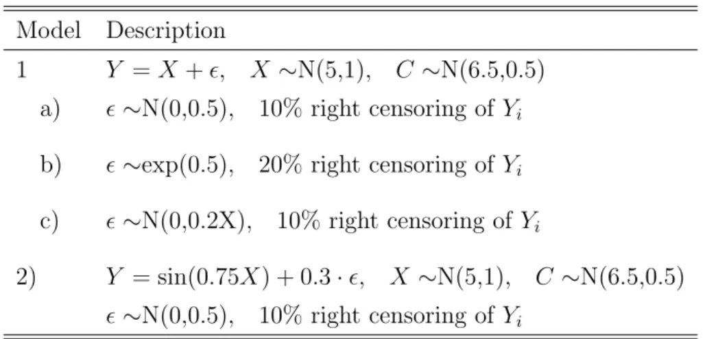
In order to investigate the properties of our estimator in presence of a censored regressor, we censor the distribution of X on both sides. νi = 0 if Xi < 3 and
νi = 10 if Xi > 7. Figure 1 illustrates the distribution of X and ν for one sample
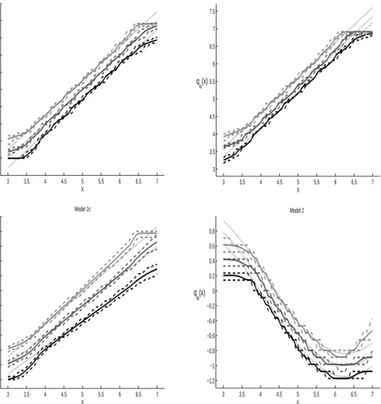
used in the simulation. 5% of the observations are on average affected by this data manipulation. Figure 2 presents the mean 0.3, 0.5 and 0.7 quantile functions as well as the 2.5%- and the 97.5%-quantile of the simulation distribution with bn = 0.1
and the true quantile functions. The estimator generally recovers the true shape of the conditional quantile functions. The bias at both sides of the support of ν is due to two reasons: first, our estimator fits locally a constant. Therefore we have
Model Description
1 Y =X+², X ∼N(5,1), C ∼N(6.5,0.5) a) ²∼N(0,0.5), 10% right censoring of Yi
b) ²∼exp(0.5), 20% right censoring of Yi
c) ²∼N(0,0.2X), 10% right censoring of Yi
2) Y = sin(0.75X) + 0.3·², X ∼N(5,1), C ∼N(6.5,0.5)
²∼N(0,0.5), 10% right censoring of Yi
Table 1: Models for simulation study.
a boundary bias that starts at a distance of the bandwidth apart of the edge of observations. Second, Gn is inconsistent below cl and above cu. This aggravates
the boundary bias but it does not affect interior estimates. Since we use the SNN smoothing we have a variable bandwidth given ν. The low density of ν at the boundaries implies a larger bandwidth given ν than in the interior of the support of
ν.
Table 2 presents the mean squared error (MSE), the squared bias and variance of the estimator for the different models. We only present the result for the median as the results for other quantiles (α = 0.3 and α = 0.7) do not differ remarkably. The MSE is calculated by using
MSE = 1 500·50 500 X k=1 50 X l=1 (ˆqk(xl)−q(xl))2.
It is apparent from the table that the estimator has the typical behaviour with respect to the bandwidth choice. In particular, there is a bandwidth which minimises the MSE. In our small numerical exercise it takes on the smallest value for bn= 0.1
Model n Bandwidth MSE Bias2 Variance 1a) 500 0.02 0.0307 0.0049 0.0258 0.1 0.0133 0.0038 0.0095 0.2 0.0436 0.0365 0.0071 5,000 0.02 0.0056 0.0019 0.0038 0.1 0.0047 0.0028 0.0019 0.2 0.0404 0.0389 0.0014 1b) 500 0.02 0.0485 0.0289 0.0197 0.1 0.0229 0.0169 0.0060 0.2 0.0541 0.0487 0.0054 5,000 0.02 0.0204 0.0175 0.0029 0.1 0.0153 0.0143 0.0010 0.2 0.0484 0.0473 0.0011 1c) 500 0.02 0.1248 0.0209 0.1041 0.1 0.0394 0.0087 0.0307 0.2 0.0395 0.0221 0.0174 5,000 0.02 0.0339 0.0211 0.0129 0.1 0.0116 0.0076 0.0041 0.2 0.0218 0.0194 0.0024 2) 500 0.02 0.0210 0.0011 0.0199 0.1 0.0039 0.0009 0.0030 0.2 0.0570 0.0034 0.0023 5,000 0.02 0.0028 0.0010 0.0018 0.1 0.0020 0.0013 0.0008 0.2 0.0046 0.0040 0.0006
1 2 3 4 5 6 7 8 9 0 50 100 150 200 250 x 0 2 4 6 8 10 0 50 100 150 200 250 300 350 ν
Figure 1: Distribution of X (left) and observed distribution of ν (right) used in the simulation study.
4
Empirical Results
We estimate conditional quantile functions with a sample of German administrative individual unemployment duration data. It is extracted from the IAB-Employment Sample 1975-2001 (IABS-R01) which contains employment trajectories of about 1.1 million individuals from West-Germany and about 200K individuals from East-Germany. It is a 2% random sample of the socially insured workforce. It contains daily information about periods of employment subject to social security taxation and periods of receipt of unemployment compensation. See Hamann et al. (2004) and Drews et al. (2006) for further details on this data such as the sampling design and the data structure. For estimation we use the same sample of unemployment spells that is used by Fitzenberger and Wilke (2007). However, we restrict the set of regressors to the age, gender and last daily wage before unemployment for all ”nonemployment” spells starting in 1996 or 1997 in West-Germany. A nonem-ployment spell contains periods of unemnonem-ployment compensation transfers and un-observed periods after an employment period. It requires at least one day of income transfers and it ends with a transition into employment. Otherwise it is right
cen-3 3.5 4 4.5 5 5.5 6 6.5 7 2.5 3 3.5 4 4.5 5 5.5 6 6.5 7 7.5 X qα(x) Model 1a 3 3.5 4 4.5 5 5.5 6 6.5 7 3 3.5 4 4.5 5 5.5 6 6.5 7 7.5 X qα(x) Model 1b 3 3.5 4 4.5 5 5.5 6 6.5 7 2.5 3 3.5 4 4.5 5 5.5 6 6.5 7 7.5 8 X qα(x) Model 1c 3 3.5 4 4.5 5 5.5 6 6.5 7 −1.2 −1 −0.8 −0.6 −0.4 −0.2 0 0.2 0.4 0.6 0.8 X qα(x) Model 2
Figure 2: Mean of the simulation estimates of the quantile functions qα(x) for
α=0.3;0.5;0.7 (from bottom to top), the 2.5%- and the 97.5%-bootstrap quantile for each estimate (dashed lines) and the true model (lighter lines) for 5,000 observations and a kernel bandwidth b= 0.1.
sored at the last observed day of income transfers. See Fitzenberger and Wilke (2004) for more details on the definition of unemployment periods in this data. Our sample comprises 21,685 observations with less than 150 individuals generating more than one spell.
We use the estimator defined in (4) to estimate smooth nonparametric condi-tional quantile functions of the distribution of unemployment duration condicondi-tional on age or previous wage level. According to our simulations, the bandwidth should not be too large or too small. After checking that the quality of our results does not change with small variations in the bandwidth, we decided to use bn = 0.1.
For the estimation of the standard errors we use the bootstrap method by drawing 500 resamples with replacement and plot the 5%− and the 95%- quantiles of the bootstrap distribution.
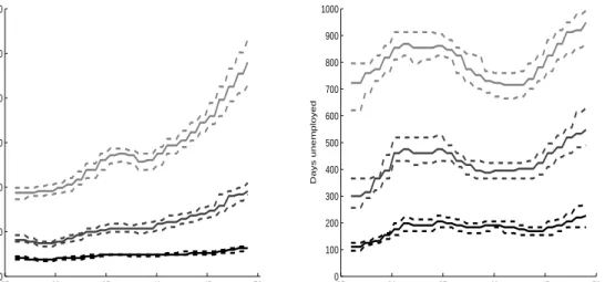
Figure 3 shows the estimation results conditional on age for the 0.3-, 0.5- and the 0.7-quantile for males (left) and females (right) with the 5- and 95%-bootstrap quantiles for each quantile. While age plays a less important role for the short-term unemployed men and women, there is a strongly positive influence of age in the group of the long-term unemployed men. The pattern for the longer unemployed women isn’t as clear as it is for men, especially not for the 0.7-quantile. According to Lechner (1997), in Germany the probability of fertility has its maximum between the age of 26 and 30 in 1995. This fact could offer a possible explanation for the peak of the curve at the age of 32: At that age, mothers have passed their maternity leave and claim remaining entitlements for unemployment benefits. However, some of them may not actually look for a job. Note that both ends of the estimated curves can have some boundary bias.
For the estimations conditional on the previous daily wage we only use the males. This is because of some lack of information about part-time work which is rather frequent for females. The histogram in figure 4 (left) shows the distribution of the variable ”previous wage”. The value ”0” means an income below and the value ”200” means an income above the social security contribution ceiling (”Beitragsbe-messungsgrenze”). For this reason we only plot results for the 10%−90%-quantile of former income. The right panel of Figure 4 shows a weakly decreasing conditional
25 30 35 40 45 50 0 200 400 600 800 1000 1200 Age (years) Days unemployed 25 30 35 40 45 50 0 100 200 300 400 500 600 700 800 900 1000 Age (years) Days unemployed
Figure 3: Estimated quantile functions conditional on age (for α = 0.3; 0.5; 0.7 from bottom to top); left: males, right: females; dashed lines: 5%- and the 95%-bootstrap quantile for each estimate.
0.3 quantile function. At the 0.5 and 0.7-quantiles, the decrease is much stronger until a previous wage level of 65 Euro per day. As discussed in detail by Fitzen-berger and Wilke (2007), the much longer long-term unemployment periods for low wage individuals are probably related with high and almost time invariant wage replacement rates. The income transfers for this group generally do not decrease after expiration of unemployment benefits as they often do not exceed the level of social benefits. It is unlikely that presented estimates have a boundary bias as we only report them in the range 20-120 EUR.
Biewen and Wilke (2005) and Fitzenberger and Wilke (2007) estimated the semi-parametric hazard rate model, the accelerated failure time model and Box-Cox quan-tile regression to similar or the same data. While there is no evident contradiction between their and our results, we claim that the estimated conditional quantile functions of this paper give more detailed insights on the conditional distribution of unemployment duration.
0 50 100 150 200 0 200 400 600 800 1000 1200
Previous daily wage (in EURO)
20 40 60 80 100 120 0 200 400 600 800 1000 1200
Previous daily wage in EURO
Days unemployed
Figure 4: left: Histogram of the previous wage for males; right: Estimated quantile functions conditional on the previous wage (forα = 0.3; 0.5; 0.7 from bottom to top) for males; dashed lines: 5%- and the 95%-bootstrap quantile for each estimate.
5
Conclusion and Outlook
This paper proposes simple nonparametric estimators for the conditional hazard rate and the conditional quantile function when the distribution of the response and of the regressor are both censored. Our simulations and our application show that these estimators are a meaningful and fast tool for data exploration that works without strong assumptions. Resulting estimates can be used for the specification of a statistical model of more structure.
There are several interesting topics for future research that may be beneficial for applied analysis: one could introduce a partially linear approach or one may establish a link to the approach of Portnoy (2004). One could allow for discrete regressors or an additive nonparametric structure. In our application we found some evidence that the conditional quantile functions possess different shapes across quantiles. Therefore one may also develop a test for shape invariance of those functions. Such a test would then provide elaborate information whether a more structural model, such as censored quantile regression, would require different model specifications
across the quantiles. It would also be straightforward to extend the estimator given in (2) to multivariate X of dimension k = 1, . . . , D by applying the idea of product kernels. The estimator for the conditional hazards rates is then
hn(y|x) = Pn i=11τi=y1di=1 Q kK µ Gn(xk)−Gn(νik) bnk ¶ Pn i=11τi≥y Q kK µ Gn(xk)−Gn(νik) bnk ¶ .
Note that this estimation strategy, however, suffers from the curse of dimensionality. For multivariate regressors see also Dabrowska (1995).
References
Akritas, M.G. (1992) Boostrapping the nearest neighbor estimator of a bivariate function. unpublished manuscript.
Akritas, M.G. (1994) Nearest neighbor estimation of a bivariate distribution under random censoring. Annals of Statistics, 22, 1299–1327.
Beran, R. (1981) Nonparametric Regression with Randomly Censored Survival Data. Technical Report, University of California, Berkeley, CA.
Biewen, M. and Wilke, R.A. (2005) Unemployment duration and the length of entitlement periods for unemployment benefits: do the IAB employment sub-sample and the German Socio-Economic Panel yield the same results?. All-gemeines Statistisches Archiv, 89(2), 409–425.
Dabrowska, D.M. (1995) Nonparametric regression with censored covariates. Jour-nal of Multivariate AJour-nalysis, 54(2), 253–283.
Drews, N., Hamann, S., K¨ohler, M., Krug, G., W¨ubbeke, C., Autorengemeinschaft ’ITM-Benutzerhandbuecher’ (2006) Variablen der schwach anonymisierten Ver-sion der IAB-Beschaeftigtens-Stichprobe 1975–2001. FDZ Datenreport 01/2006. Fan, J. (1992) Design-adaptive Nonparametric Regression. Journal of the
Fitzenberger, B. and Wilke, R.A. (2004) Unemployment Durations in West -Germany Before and After the Reform of the Unemployment Compensation System dur-ing the 1980ties. ZEW Discussion Paper 04-24.
Fitzenberger, B. and Wilke, R.A. (2006) Using Quantile Regression for Duration Analysis. Allgemeines Statistisches Archiv, 90(1), 103–118.
Fitzenberger, B. and Wilke, R.A. (2007) New Insights on Unemployment Duration and Post Unemployment Earnings in Germany: Censored Box-Cox Quantile Regression at Work. ZEW Discussion Paper 07-007.
Hamann, S., Krug, G., K¨ohler, M., Ludwig-Mayerhofer, W. and Hacket, A. (2004) Die IAB-Regionalstichprobe 1975-2001: IABS-R01. ZA-Information 55, S. 36-42
Kaplan, E. L., and P. Meier (1958) Nonparametric estimation from incomplete observations. Journal of the American Statistical Association, 53, 457–481. Koenker, R. and Bilias, Y. (2001) Quantile Regression for Duration Data: A
Reap-praisal of the Pennsylvania Reemployment Bonus Experiments. Empirical Economics, Vol.26, 199–220.
Koenker, R. and Geling, O. (2001) Reappraising Medfly Longevity: A Quantile Re-gression Survival Analysis. Journal of the American Statistical Association, Vol.96, No.454, 458–468.
Lechner, M. (1997) Eine empirische Analyse der Geburtenentwicklung in den neuen Bundesl¨andern. Beitr¨age zur angewandten Wirtschaftsforschung, No. 551-97. Machado, J.A.F. and Portugal, P. (2002) Exploring Transition Data through Quan-tile Regression Methods: An Application to U.S. Unemployment Duration. In:
Statistical data analysis based on the L1-norm and related methods – 4th
In-ternational Conference on the L1-norm and Related Methods (Ed. Yadolah
McKeague, I.W. and Utikal K.J. (1990) Inference for a Nonlinear Counting Process Regression Model. Annals of Statistics, 18, 1172–1185.
Portnoy, S. (2004) Censored Regression Quantiles. Journal of the American Sta-tistical Association, Vol.98, No.464, 1001–1012.
Stone, C.J. (1977) Consistent nonparametric regression. Annals of Statistics, 5, 595–645.
Van Keilegom, I. (1998) Nonparametric Estimation of the Conditional Distribu-tion in Regression with Censored Data. Ph.D. Thesis, Limburgs Universitair Centrum, Belgium
Van Keilegom, I. and Veraverbeke, N. (2001) Hazard Rate Estimation in Non-parametric Regression with Censored Data. Ann. Inst. Statist. Math., 53, 730–745.
Yang, S. (1981) Linear functions of concomitants of order statistics with appli-cations to nonparametric estimation of a regression function. Journal of the American Statistical Association, 76, 658–662.
Nr. 9/2007
Imprint
No. 9/2007
Publisher
The Research Data Centre (FDZ) of the Federal Employment Service in the Institute for Employment Research Regensburger Str. 104
D-90478 Nuremberg
Editorial staff
Stefan Bender, Dagmar Herrlinger
Technical production
Dagmar Herrlinger
Copyright
Reproduction – also in parts – only with permission of the FDZ Download http://doku.iab.de/fdz/reporte/2007/MR_09-07.pdf Internet http://fdz.iab.de/ Corresponding author Laura Wichert
University of Konstanz, Department of Economics, Box D 124, 78457 Konstanz, Germany