SEQUENTIAL CLUSTERING VIA RECURRENCE
NETWORK ANALYSIS
by
Zhang Zhang
B.S. in Statistics, Wuhan University, 2010
M.A. in Statistics, University of Pittsburgh, 2012
Submitted to the Graduate Faculty of
the Kenneth P. Dietrich School of Arts and Sciences in partial
fulfillment
of the requirements for the degree of
Doctor of Philosophy
University of Pittsburgh
2017
UNIVERSITYOFPITTSBURGH DIETRICH SCHOOL OF ARTS AND SCIENCES
This dissertation was presented
by
Zhang Zhang
It was defended on
Dec 06, 2017
and approved by
Satish Iyengar, PhD, Department of Statistics
Wilbert Van Panhuis, PhD, Department of Epidemiology
Kehui Chen, PhD, Department of Statistics
Yu Cheng, PhD, Department of Statistics
Copyright cby Zhang Zhang 2017
SEQUENTIAL CLUSTERING VIA RECURRENCE NETWORK ANALYSIS Zhang Zhang, PhD
University of Pittsburgh, 2017
In this dissertation, we propose a new sequential clustering method based on nonlinear dynamic theories and exponential random graph models (ERGMs), a class of social network models. In particular, we convert each sequence to its recurrence network and make use of the flexibility and information of the network. Our algorithm shows good performance on simulated data, real-world data and public benchmark data based on clustering evaluation metrics.
To make sure the connection between a sequence and a network is reliable, we also conduct a study to examine whether the network contains enough information of the original sequence. We consider recurrence networks as images and build state of the art convolutional neural network (CNN) models based on image data to predict the labels of original sequences. Our method is very competitive compared with other advanced sequential classification methods. This also ver-ifies that recurrence networks are very informative and give us enough information for real-world applications.
Keywords: Sequential clustering; Nonliear dynamical systems; Recurrence networks; Exponen-tial random graph models; Recurrence image classification; Convolutional neural networks.
TABLE OF CONTENTS
1.0 INTRODUCTION . . . 1
2.0 SOME SEQUENTIAL CLUSTERING APPROACHES . . . 3
2.1 Baseline Approaches . . . 3
2.2 ARIMA based Approaches . . . 4
2.3 HMM based Approaches . . . 4
2.4 Other Approaches . . . 5
3.0 BACKGROUND . . . 7
3.1 Nonlinear Dynamic Systems . . . 7
3.2 Recurrence Plot and Recurrence Network . . . 8
3.3 Recurrence Image . . . 11
4.0 SEQUENTIAL CLUSTERING VIA RECURRENCE NETWORKS AND EXPO-NENTIAL RANDOM GRAPH MODELS . . . 12
4.1 Exponential Random Graph Models . . . 12
4.2 Proposed Method . . . 13
4.2.1 Testing of Nonlinear Dynamics . . . 14
4.2.2 Construction of Recurrence Plots . . . 16
4.2.3 ERGM Model Terms . . . 17
4.2.4 Method Evaluation . . . 19
4.3 Recurrence Network Analysis for ARMA models . . . 21
4.4 Simulation Study . . . 24
4.5 Application . . . 28
4.5.2 UCR Time Series Data . . . 29
5.0 HOW MUCH INFORMATION IS CONTAINED IN A RECURRENCE NET-WORK? . . . 37
5.1 Motivation . . . 37
5.2 Introduction . . . 37
5.3 Related Work . . . 39
5.4 Proposed Method . . . 40
5.4.1 Recurrence Images and Why CNN Works . . . 40
5.4.2 Image Scaling and Data Augmentation . . . 41
5.4.3 CNN Architectures . . . 43
5.5 EXPERIMENTAL EVALUATION . . . 46
5.5.1 Model Configuration . . . 46
5.5.2 Performance Evaluation . . . 46
5.6 Conclusions and Future Work. . . 54
LIST OF TABLES
1 Accuracy rates of different methods, using U(-0.1,0.1) noise . . . 25
2 Adjusted Rand Index of different methods, using U(-0.1,0.1) noise . . . 25
3 Accuracy rates of different methods, using U(-0.2,0.2) noise . . . 25
4 Adjusted Rand Index of different methods, using U(-0.2,0.2) noise . . . 25
5 Performance comparison of different methods . . . 35
6 Performance evaluation on Coffee Data . . . 35
7 Performance evaluation on Gun Point Data . . . 36
8 Performance evaluation on Wafer Data . . . 36
9 Performance evaluation on FaceFour Data . . . 36
10 Performance evaluation on CinC ECG Data . . . 36
11 Summary of the CNN network 1. . . 44
12 Summary of the CNN network 2. . . 45
13 Datasets information and optimal model hyperparameters . . . 52
LIST OF FIGURES
1 Four common patterns of recurrence plots . . . 10
2 Upper left: Ulam map time series; upper right: square of AR(1) time series; lower left: surrogate nonlinearity testing of Ulam map; lower right: surrogate nonlinearity testing of square of AR(1). . . 15
3 Four points lines: Simulation results of mean edge density for= 0.05, 0.1, 0.2, 0.3; Four solid lines: The real mean edge density for= 0.05, 0.1, 0.2, 0.3 . . . 23
4 Top: RN-ERGM clustering; bottom: raw sequences with Euclidean distance . . . . 26
5 Top: LPC cepstral coefficients clustering; bottom: correlation based clustering by Kollias . . . 27
6 Mutual information againstτ of 46 sequences . . . 30
7 FNN statistics againstmof 46 sequences . . . 31
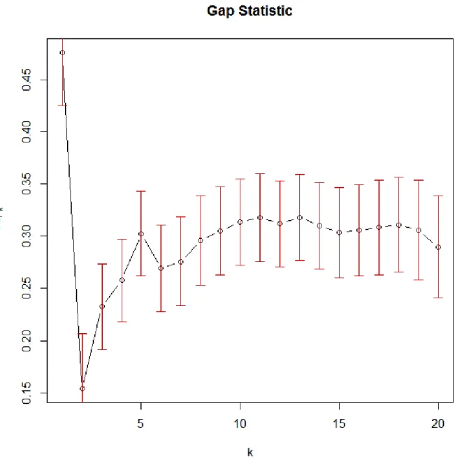
8 Gap statistic . . . 32
9 Map of clustering by RN-ERGM approach . . . 33
10 Map of clustering by dynamic time warping distance . . . 33
11 Map of clustering by Maharaj model-based Dissimilarity . . . 34
12 Map of clustering by Piccolo model-based Dissimilarity . . . 34
13 Recurrence images and time series of class mean for Coffee . . . 47
14 Recurrence images and time series of class mean for Wafer . . . 48
15 Recurrence images and time series of group mean . . . 49
16 Recurrence images and time series of class mean for GunPoint. . . 50
1.0 INTRODUCTION
Benefiting from rapid development of technology, sequential data have been collected and ana-lyzed in more and more domains with different goals. In contrast with common static data in feature space, sequential data usually has dynamic properties. If we regard each sequence as an observation point and each time stamp as a coordinate, sequential data also has high dimensions in general. In addition, all the components are temporal and many of them are highly correlated.
Sequential clustering, as an unsupervised learning task, has been shown to be effective in providing useful information in various domains such as biology Ernst et al.(2005), ecology Li et al. (2001), astronomy Ng and Huang (1999), finance Maharaj (2000), economics Van Wijk and Van Selow(1999) and information scienceNiennattrakul and Ratanamahatana(2006). It can help us gain insight into the mechanisms that generate the sequences and find common features for each cluster. Although sequential clustering is very important, there is little literature on sequential clustering as sequential classification. This may result from the fact that we do not have ground truth for clustering analysis. It is harder to evaluate performance of clustering analysis on some benchmark data sets.
There are several different ways to consider and process sequential data, such as time series, longitudinal data and functional data. The goals and models used in these different areas not only share some common elements but also have many differences. Nonlinear dynamic time series is a subclass of time series that is based on nonlinear dynamical systems and chaos theory. Although it is called time series, the models used here are quite different from some common time series models such as ARIMA and GARCH which are widely used. An observed nonlinear dynamic time series is considered as a sequence of scalar measurements which is a projection of a trajec-tory in a nonlinear dynamic system. Nonlinear dynamic theory regards the stochastic element as a small contamination of an essentially deterministic, nonlinear process. Many sequential
cluster-ing approaches work well for linear time series and linear systems. However, many systems are nonstationary and nonlinear in real-world problems. And those powerful linear tools usually do not work well for these systems. To the best of our knowledge, there is no literature on sequential clustering based on rigorous nonlinear dynamic theories.
With the emergence of online network communities, such as Facebook, Twitter and LinkedIn, social network analysis has become one of the fastest growing fields in recent years. Social network analysis is used to investigate social structures through the use of networks and graph theory. It characterizes networked structures in terms of nodes and edges.Goldenberg et al.(2010) provided an overview of many models and techniques in this field.
In this thesis, we propose a sequential clustering method based on social network models. In particular, the proposed method is based on nonlinear dynamic theory and recurrence network anal-ysis (RNA) using exponential random graph models (ERGM). The main steps of the method are as follows: we would convert the nonlinear time series into a recurrence plot, which is equivalent to a conversion to an adjacency matrix. ERGMs, with appropriate network statistics, are fitted and selected for each adjacency matrix, and the sequential clustering are completed based on ERGM profiles (model coefficients).
The rest of the dissertation is organized as follows: In Chapter 2, we review some previous methods in the field. Chapter 3 gives the related definitions and background techniques for our research including nonlinear dynamics, recurrence plots and recurrence images. Chapter 4 is de-voted to our proposed sequential clustering method in detail, with a simulation study, real-world application and benchmark datasets evaluation. Chapter 5 conducts a study to check whether recur-rence networks contain enough information from the original sequences via corresponding image classification. It also provides a tool for common sequential classification tasks.
2.0 SOME SEQUENTIAL CLUSTERING APPROACHES
Clustering is to organize unlabeled subjects into homogeneous groups using algorithms and dis-tance (similarity) measures. There has been a lot of literature written concerning sequential clus-tering over the past 20 years. Liao(2005),Rani and Sikka(2012) provided fairly complete surveys about sequential clustering from the perspective of time series. McNicholas and Murphy(2010),
Kom´arek et al.(2013) andCoffey et al.(2014) focused on clustering longitudinal data which usu-ally refers to shorter sequential data.
2.1 BASELINE APPROACHES
It is hard to enumerate all sequential clustering approaches due to the extensive of literature in this field. It is even difficult to classify all those approaches perfectly. Here we will discuss some of the most popular ones. Perhaps, the most common but simplest class of approaches is to use the traditional clustering algorithms for static data on the raw sequential data directly. By doing so, each temporal measurement of the sequence is considered a feature of that subject. The most commonly used algorithms in this category are K-means, hierarchical clustering and spectral clustering. Euclidean distance is chosen as the dissimilarity measure in most of cases. Many researchers still use traditional clustering methods on raw data. Sometimes they do provide adequate results. Although traditional algorithms often provide acceptable performance in certain cases, they usually do not provide a reasonable interpretation. They are hardly considered the best choice in one’s toolbox. They are often considered baseline approaches instead.
2.2 ARIMA BASED APPROACHES
One traditional class of approaches is based on the Autoregressive Integrated Moving Average (ARIMA) models, considered classical time series models. Piccolo (1990), Maharaj (2000) ,
Baragona (2001) and Kalpakis et al. (2001) did time series clustering based on ARIMA mod-els. Although their approaches varied in their details, they had similar ideas. Given a time series, an ARIMA or subclass of ARIMA model was fit based on their autocorrelation function (ACF) and partial autocorrelation function (PACF). Then a distance measure was built based on either fitted ARIMA coefficients or residuals by Euclidean distance or p-value of an appropriate hypoth-esis test. Finally, traditional clustering algorithms such as hierarchical clustering were used on the pairwise distance matrix to get homogeneous groups. This class of approaches has very rigorous and extensive theoretical foundation due to our thorough understanding of ARIMA models and experience with them in time series analysis. Although this class of approaches performs well in many simulation studies, it does not perform well on many read-world data sets. In fact, the naive baseline approaches sometimes outperform this class of approaches in some applications based on our test.
Bad performance may be due to several reasons. First of all, this class of approaches is very sensitive to nonstationarity. The integrated parameter cannot always cope with some complicated global trends well. However, purely stationary time series are hard to observe in real world prob-lems. Secondly, fitting an ARIMA model is sometimes fairly subjective. Although some R pack-ages fit a group of ARIMA models automatically, the generated ARIMA orders may not be the ones the users select themselves via ACF and PACF. In general, lower order models are preferred if several models are comparable. However, lower order models also give smaller sets of coeffi-cients. They might make some time series hard to separate from others.
2.3 HMM BASED APPROACHES
Hidden Markov Models (HMM) are another class of model - based approaches. HMM assumes that the observed sequence is governed by an unobserved sequence which follows a Markov
pro-cess. It has the advantage of modeling state changes in sequential data, thus sequence clustering with HMM is of interest to many researchers. Smyth et al. (1997) first used HMM in sequential clustering. HMM was fit to each sequence to obtain the transition matrix and emission parame-ter estimates. For each pair of sequences, the log-likelihood of one sequence given the estimated transition matrix and emission parameters of another sequence was calculated. The symmetrized log-likelihood was used to measure the dissimilarity between two sequences. Finally hierarchi-cal clustering was applied on the resulting distance matrix. Other researchers considered various metrics to compute the distance or similarity between HMM sequences. Panuccio et al. (2002) developed a model-based method and Bicego et al. (2003) proposed a similarity-based method.
Jebara et al.(2007) combined spectral clustering with the mixture of HMM.Coviello et al.(2014) proposed a variational hierarchical EM algorithm for clustering HMM, using the parameters to characterize the cluster centers.
Perhaps HMM is the class of models that statisticians, computer scientists and engineers all accept. It not only has mature model-based theoretical foundation but also performs well in many applications in the machine learning and data mining community. However, this class still has several limitations. Firstly, the number of states of an unobserved sequence is not easy to confirm without further study. For many problems, a finite number of states does not exist, but is a useful conceptualization only. Moreover, the assumption of Markov property may not be satisfied for given data and almost all of applications only considered using a first-order model which may not be the best choice. Finally, this class does not scale well for large data problems.
2.4 OTHER APPROACHES
In addition to those two model-based classes of approaches mentioned above, there are also many nonparametric or data driven approaches. Sakoe and Chiba (1978) first proposed a dynamic time warping (DTW) algorithm. It is a parameter free approach initially used for speech recognition. The basic idea is to find out an optimal match between two given sequences with certain restric-tions. DTW also has several variants proposed byKahveci and Singh(2001),Kahveci et al.(2002),
cluster-ing approaches based on frequency domain. Vlachos et al.(2003) presented an approach to per-form incremental clustering of time series at various resolutions using the Haar wavelet transper-form.
De Lucas(2010) considered a distance measure based on the integrated periodograms. There does not exist an approach that could outperform all other approaches. In this thesis, we will focus more on model-based approaches.
3.0 BACKGROUND
3.1 NONLINEAR DYNAMIC SYSTEMS
The nonlinear dynamic time series discussed in this thesis is mainly based on the theory of dynami-cal systems. Compared with common stochastic linear time series models, nonlinear dynamic time series can be regarded as an essentially deterministic, nonlinear process with some small stochas-tic elements. We could also consider a purely determinisstochas-tic system as a limiting case of a Markov process on a continuum of statesKantz and Schreiber(2004).
We will first introduce some notation for dynamical systems in phase space. Consider a state vectorx ∈ Rm. The dynamical systems can be defined either by an m dimensional map in the discrete case:
xn+1 =F(xn), n ∈ Z
or in the continuous case:
d
dtxt=f(xt), t∈ R
The solutions of the differential equations above are called trajectories of the dynamical systems. In the autonomous case, the trajectory is known to exist and to be unique if the vector field f is Lipshitz continuous, given the initial conditions. The behavior of the trajectory depends on bothf
orF and initial conditionsx(0)orx0. The observation of a real system usually does not generate
all possible state variables. Not all of them can be measured or are visited by the process up to that time. Usually only one scalar sequenceunis available:
un =u(x(n4t)) +εn
That means we can only observe the dynamic system through some measurement functionuwith some random noiseεn. We therefore have to convert the observations into state vectors through
phase space reconstruction Abarbanel et al. (1993). The most commonly used method is to re-construct a time delay trajectorys(t): si = (ui, ui+τ, ..., ui+(m−1)τ)T, where m is the embedding dimension andτ is the time delay parameter. Takens(1981) pointed out that ifm ≥ 2d+ 1, the topological structure of the original trajectory can be preserved, where dis the dimension of the underlying attractor.
Both embedding parameters, the dimensionmand the delayτ, have to be chosen carefully. A precise knowledge ofmis desirable since we want to exploit determinism with minimal computa-tional effort. Ifmis too small, the assumption of Taken’s embedding theorem is unlikely to satisfy, i.e. the topological property of reconstructed systems may be different from the original systems. If m is too large, not only will the computational cost be too expensive, but also the redundant information will degrade the performance of clustering or other related algorithms. Kennel et al.
(1992),Kantz and Schreiber(2004),Cao(1997) proposed approaches for the determination ofm. A good estimate of the delay parameter τ might be more difficult to obtain. Random noise and temporal correlations can lead to a linear dependence between the successive components. Therefore the delay has to be chosen in a way that such dependence vanishes. However, ifτ is too large, successive components become almost independent, and we will lose too much information.
3.2 RECURRENCE PLOT AND RECURRENCE NETWORK
In this section, I will briefly introduce the recurrence plot (RP) and its connection with a network. An RP is an advanced analysis technique for nonlinear dynamic time series, which was first intro-duced byEckmann et al.(1987). It is a graph of a square distance - like matrix in which the matrix elements correspond to those times at which a state of a dynamic system recurs. Technically, the RP shows all the times when the phase space trajectory visits roughly the same area in the phase space. Formally, it is defined as a matrix:
Ri,j(ε) = Θ(ε− ||xi−xj||), (3.1) where|| · ||is a suitable norm (usually the Euclidean norm) in the considered phase space,Θ(·)is the Heaviside function andεis a threshold parameter that is reasonably small.xiis the phase space
vector observed at timeifor the trajectoryx(t). As mentioned in last section, usually we can only observe a scalar time series u(t) and need to use the embeddingsi = (ui, ui+τ, ..., ui+(m−1)τ)T, wheremis the embedding dimension andτ is the time delay parameter.
Equation 3.1 shows that a recurrence is defined as a state xj is sufficiently close to xi. The threshold distanceε defines how close we think ”sufficiently close” is, i.e., if xj falls into an m-dimensionεball ofxi, xj is a recurrence point ofxi. εis a crucial parameter in the RP analysis. Ifεis too small, many recurrences and recurrence structures will be lost. On the other hand, if ε
is too large, redundant information or random noise will distort any existing structure in the RP. In general, the optimal choice ofεdepends on the applications and heuristic studies, but a smaller threshold is desirable in most of cases.
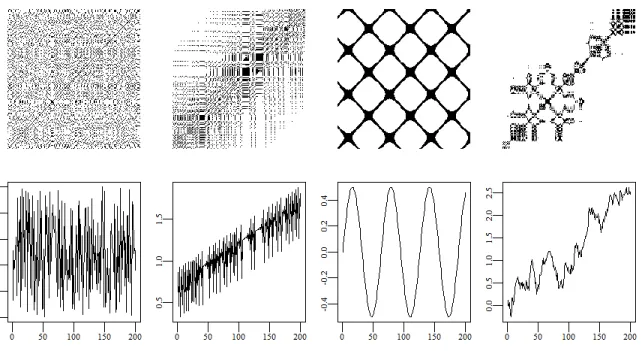
The original purpose of RPs was to visualize higher dimensional phase space trajectories. Structural patterns in RPs reveal hints about the dynamics of these trajectories. RPs can be not only used on noisy data, but also applied to nonstationary data. The RPs show characteristic large scale and small scale patterns. From left to right, Figure1 shows four common patterns of recurrence plots, from left to right: homogeneous (uniformly distributed noise), drift (logistic map with linear global trend), periodic (sine function) and disrupted (Brownian motion). The length of all four time series areN = 200. No embeddings are used and the thresholds areε = 0.1. In the plots, a pixel shows black when the correspondingRi,j(ε) = 1.
In addition to global structures, RPs can also show local structures which consist of a combi-nation of isolated dots (chance recurrences), dots forming diagonal lines (deterministic structures) as well as vertical/horizontal lines or dots clustering to inscribe rectangular regions (laminar states, singularities). These local structures are the basis for network analysis of the RPs. In fact, RPs preserve all topological properties of the system, such that we can reconstruct a time series from its recurrence matrix (Thiel et al.,2004a), (Robinson and Thiel,2009).
The recurrence matrixR(ε)can be converted to an adjacency matrix naturally:
Y(ε) = R(ε)−IN, (3.2)
whereY(ε)is the adjacency matrix representation of some undirected binary network. It is easy to see that this conversion in fact just removes the self-similarity in the undirected network. Thus all the topology properties and dynamics are preserved. A RP is equivalent to a undirected unweighted
Figure 1: Four common patterns of recurrence plots
network. The advantage of doing recurrence network analysis (RNA) is that we can currently deal with a dynamic system as a complex network, where plenty of network statistics, theories and models are available. Donner et al.(2010),Marwan et al.(2009) tried to connect network statistics and recurrence plots. However, their works only discussed some common network descriptive statistics without any model settings.
Moreover, the definition of recurrence networks should not be confused with recurrent neural networks (RNN), a class of artificial neural networks where connections between units form a directed cycle. In recurrence network, each node denotes a time point subject while each edge denotes the revisiting property of the trajectory. Recurrence networks are used to study the global and local relationship between different time nodes. However in a recurrent neural network, each node denotes a mathematical function whose inputs are some transformations of variables. In other words, a recurrence network is a special case of social network while a recurrent neural network is a special case of graphical model. We will study time series and their corresponding recurrence networks from the perspective of social network models in Chapter 3.
3.3 RECURRENCE IMAGE
In the last section, we showed that a recurrence plot (RP) is equivalent to an undirected binary net-work. A natural question arises: How much information is contained in a RP?Thiel et al.(2004b) discussed this problem. They stated that under some conditions, it is possible to reconstruct an attractor of a dynamical system from the recurrence plot, at least topologically. However, they admitted the results are of mainly theoretical relevance. We want to study this problem from a practical perspective: can we use the information of a RP to solve some real-world time series related tasks, such as time series classification? If we could classify time series purely using recur-rence plots with high accuracy compared with other time series classification algorithms, we could quite confidently say that recurrence plots contain enough information and even more than its time domain form of the original time series.
The binary edges of RPs come from setting the threshold parameter which could help reduce noise. This also leads to unavoidable information loss, although some methods for efficiently choosing hyperparameters have been proposed to minimize the loss. To make the problem some-what easier, we would use unthresholded RPs, i.e., weighted recurrence networks, as our input training data. To differentiate these with original RPs which are binary networks, we will call them recurrence images since each edge in a weighted network has a continuous value like a pixel in an image. We will study time series and their corresponding recurrence networks from the perspective of image recognition in Chapter 4.
4.0 SEQUENTIAL CLUSTERING VIA RECURRENCE NETWORKS AND EXPONENTIAL RANDOM GRAPH MODELS
In this chapter we will first introduce exponential random graph models (ERGMs) in section 4.1. Then we will propose our sequential clustering method which is based on recurrence networks and exponential random graph models (RN-ERGM hereafter) in section 4.2. Our method is initially intended for clustering of nonlinear dynamic time series. Although we will use a surrogate data testing method to test nonlinear dynamics of the sequences for reference, it is generally very hard to judge whether the data are generated from linear stochastic models like ARIMA models, or from nonlinear dynamic systems. Moreover linear stochastic time series can be considered as a special case of nonlinear dynamic time series with much noises. Thus we will try to connect our proposed method with linear stochastic time series and check the robustness of our method in section 4.3. Section 4.4 presents some simulation results. In section 4.5, a case study about measles time series clustering is presented followed by applying our proposed method on several famous benchmark data sets.
4.1 EXPONENTIAL RANDOM GRAPH MODELS
Exponential random graph models (ERGMs) are a family of statistical models for analyzing net-work data. Since they are the basis of our clustering algorithm, we will introduce it first in this section. Frank and Strauss(1986) proposed the following characterization for the probability dis-tribution of undirected networks:
P(Y =y) = exp n−1 X k=1 θkSk(y) +γT(y) +c(θ, γ) ! , (4.1)
where y is the observed adjacency matrix, θks and γ are parameters, c(θ, γ) is the normalizing constant, the statisticsSkare the number ofk-stars andT is the number of triangles defined as:
Sk(y) = X 1≤i≤n yi+ k ! , T(y) = X 1≤i≤j≤h≤n yijyihyjh
Here yi+ is the centrality degree of ith node. Whenk = 1, S1(y)degenerates to the number
of edges in the network. Frank and Strauss(1986) used primarilyS1(y) andS2(y), i.e. they set
θk = 0fork ≥3. Although the models fairly look like the common generalized linear regression models (GLMs) with exponential family, they are quite different. In GLMs, all covariates might be correlated, but they are observed separately. In network models above, all covariates are dependent since they are different statistics calculated from the same adjacency matrix.
Wasserman and Pattison (1996) proposed a generalized class of network models that is the current formulation of Exponential Random Graph Models (ERGM):
P(Y =y) =expθTu(y)−φ(θ), (4.2) whereu(y)can be a vector of any network statistics andφ(θ)is the normalization constant. This setting highly extends ERGM family and makes this class of models more flexible. Morris et al.
(2008) summarized most commonly used ERGM statistics. The estimation of ERGMs is not a trivial problem due to normalization constant. Snijders(2002) proposed a MCMC based method to estimate parameters in ERGMs. Hunter et al. (2008) estimated likelihood ratios for nearby θi using a MCMC procedure related to the work ofGeyer and Thompson(1992).
4.2 PROPOSED METHOD
The steps of our proposed RN-ERGM sequential clustering method are summarized below:
(1) Given a set of sequences, test whether each sequence has nonlinear dynamic structure against null hypothesis that the sequence is a linear stochastic process.
(2) Construct recurrence plots and then recurrence networks for all sequences with selected em-bedding parametersm, time delay parameterτ and threshold distanceε.
(3) Fit an ERGM for each sequence and obtain a vector of ERGM parameter estimates. For N se-quences, there are N vectors of parameter estimates. Build a distance (affinity) matrix, where each entry is the distance (similarity) between each pair of vectors of estimates. Apply hi-erarchical clustering (spectral clustering) on the obtained distance (similarity) matrix to get clusters.
We will show the details of each step in following.
4.2.1 Testing of Nonlinear Dynamics
Given a set of time series, the first step is to confirm whether they are linear stochastic processes or nonlinear dynamic time series. For former cases, we should always try linear approaches first, since linear approaches are more mature and interpretable. For latter cases, our approaches will work better. The hypothesis testing we need to do is:
H0: the time series is a Gaussian linear process
Hα: the time series is a nonlinear dynamic time series
We will use the surrogate data testing first proposed by Schreiber and Schmitz (2000). The test is implemented by generating several surrogate data according to H0 and comparing the values
of a discriminating nonlinear statistic between the original data and the surrogate data. If the statistics value of original series are far from the surrogate ones, the null hypothesis is rejected and nonlinearity is concluded.
Generating surrogate data sets is a challenging step. Adequate surrogate data sets must contain correlated random numbers which have the same power spectrum as the original data. This is the case if the Fourier transforms of the original data and the surrogates differ only in their phases but have the same amplitudes which go into the power spectrum. Roughly speaking, we will generate a surrogate time series that has almost the same power spectrum as original data and also follows Gaussian assumption, by using fast Fourier transform (FFT) and phase randomization.
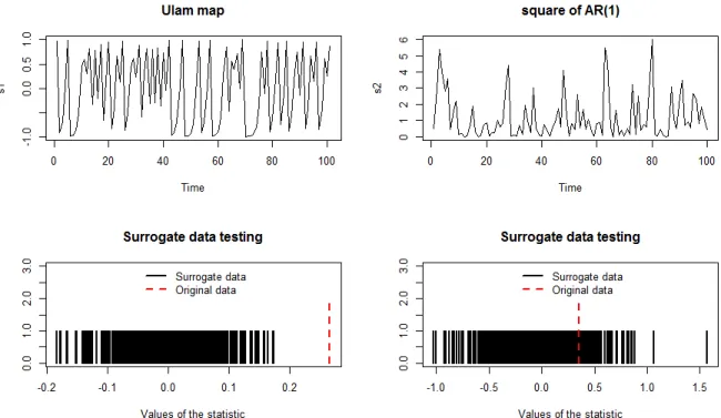
Consider the example in Figure2. We simulate two time series: the first one is a Ulam map, a special case of logistic map:
Figure 2: Upper left: Ulam map time series; upper right: square of AR(1) time series; lower left: surrogate nonlinearity testing of Ulam map; lower right: surrogate nonlinearity testing of square of AR(1).
The second one is a quadratic transformation of AR(1):
yn =a2n, an = 0.5an−1+ηn
From the two bottom graphs in Figure 2, we can observe that the test for Ulam map is sig-nificant, while for the square of AR(1) is not. Although we did a quadratic transformation for a AR(1) time series, there is still no nonlinear dynamics in the process, i.e., all the dynamics are contained in the linear AR(1) part and the nonlinearity is purely static. This illustrates the surro-gate testing works well when we want to differentiate nonlinear dynamics and common nonlinear transformation of linear processes.
4.2.2 Construction of Recurrence Plots
To construct recurrence plots and then recurrence networks for all sequences, we need to select the embedding parameterm, time delay parameterτ and threshold distanceεappropriately. Since we have a set of sequences, those parameters should be at a global level, otherwise, the comparison of generated networks will be unfair.
For embedding parameterm, the basic idea is that by decreasing them an increasing amount of phase space points will be projected into the neighborhood of any phase space point. Points whose coordinates which are eliminated by the projection differ strongly, are good candidates for false neighbors in the lower dimensional space (Kantz and Schreiber, 2004). More formally, for each point of the time series, we could take its closest neighbor inmdimensions, and compute the ratio of the distances between these two points inm+ 1dimensions and inmdimensions. If the ratio is larger than a thresholdr, the neighbor is false:
Xf nn(r) = PN−m−1 n=1 Θ |s(nm+1)−s( m+1) k(n) | |s(nm)−s(km(n))| −r ! Θσr − |s(m) n −s (m) k(n)| PN−m−1 n=1 Θ σ r − |s (m) n −s(km(n))| , (4.3)
where s(km(n)) is the closest neighbor to sn in m dimensions. From our experience in simulation studies and real-world cases, the embedding dimensions are usually overestimated. Heuristic study helps a lot in choosing embedding parameters. Since we have a set of sequences, we usually
would choose an embedding parameter that gives both small Xf nn(r) and smaller Xf nn(r)than
Xf nn(r−1)for most of sequences.
For time delay parameterτ, we would choose it by calculating the mutual information (Fraser and Swinney,1986): I(τ) = − X ui,ui+τ pui,ui+τ(τ) log pui,ui+τ(τ) puipui+τ (4.4)
The mutual information here measures the average shared information between current timeiand a later delay time i+τ. Smaller value means that we could not get too much information for a latter delay time given current values. Thus we should take theτwhereI(τ)is fairly small. Again, this approach tends to give overestimates of the delay time parameter. We will choose the smallest
τ among estimatedτ’s of all sequences.
For the threshold distance parameter ε, several works have given some ideas for choosing it (Thiel et al., 2002), (Matassini et al., 2002), (Marwan et al., 2007), however a general and systematic solution on the remains an open task for future work. For our specific clustering task with ERGM, we need to consider what kinds of values that could fit ERGM well. More specifically, we would like to chooseεthat matches the ERGM terms well. In general, the values should make the edge density of a network less than1%and make the degree distribution highly right skewed, i.e., we tend to use lower order centrality degree to represent a network.
4.2.3 ERGM Model Terms
There are a lot of available model terms in ERGMs. In fact, any network statistics can be consid-ered as predictors and put into ERGMs in the model setting. It is very hard to use a global model selection algorithm or a stepwise model selection algorithm. First, there can be infinite network statistics in principle. Second, the network statistics can be highly dependent. The selection of model terms is mainly based on both heuristic study and some goodness-of-fit statistics. However, not all network statistics are appropriate to represent the networks. Since we are talking about recurrence networks, we tend to use network statistics that have direct or indirect interpretations in theory of nonlinear dynamics. Here we will talk about some network statistics that we use in our models.
The edge density, ˆ ρ(ε) = 1 N(N −1) N X i,j=1 Yi,j(ε) (4.5)
is defined as the average of the degree densities of all nodes and characterizes the proportion of possible edges that are present in the network. It is easy to show that ρˆ(ε) is a monotonically increasing function of the threshold parameterε. It also can be interpreted as the recurrence rate of the underlying trajectory.
The edge density is one very important term. Since it has a direct connection with correlation dimension of the system:
D = lim
ε→∞Nlim→∞
∂ln ˆρ(ε)
∂lnε . (4.6)
Correlation dimension is one commonly used type of fractal dimensions to characterize dynamic systems. It is an invariant nonlinear statistic, i.e., its value would not change under smooth trans-formations such as state space reconstructions. Although edge density is not an invariant statistic, it still provides some information about the correlation dimension.
The centrality degree of a nodev in an undirected network is:
ˆ kv(ε) = N X i=1 Riv(ε) (4.7)
We could then use the number ofk-degree statistics:
d(k) =
N
X
i=1
I(ˆki(ε) =k), (4.8)
whereI(·)is an indicator function. d(k)calculates the number of nodes in the network of degree
k. Using bothk-degree statistics and edge density, we could represent a network in edge-level. Another type of network statistics are path-level statistics. A commonly used one is the average path length: ˆ L(ε) = 2 N(N −1) X i<j li,j(ε), (4.9)
whereli,j(ε)is the shortest path length between time pointiandjgivenε. The shortest path length is set to zero for disconnected pairs of nodes. AlthoughDonner et al.(2010) pointed out that the zero length definition has no major impact on the corresponding statistics, it would be biased when characterizing a network. In recurrence networks, if the distance between two states is small, there would be a short path between them. However if the distance is large, the path length between two
states becomes zero by this definition. That contradicts the monotonicity. We will use a more local path-level statistics instead:
l2 =
N
X
i<j<k
RijRjk (4.10)
This statistic will calculate the number of paths that have length 2 in the network.
Most of the network statistics above characterize the geometric instead of dynamical properties of underlying systems. (Marwan et al., 2007) summarized some recurrence quantification (RQ) statistics that could characterize the dynamical properties. Those statistics in general are not used in ERGM models and some of them would make model degenerated in our experiments. However, the histogram of the lengths of the diagonal structures in the RP is one important RQ statistics that contributes to our method. It is defined as:
HD(l) = N X i,j=1 (1−Ri−1,j−1) (1−Ri+l,j+l) l−1 Y k=0 Ri+k,j+k, (4.11) whereldenotes the length of diagonal lines in the recurrence plot. If the trajectory visits the same region of the phase space multiple times at different time stamps, the count of diagonal lines would increase. The diagonal line length is determined by the duration of such similar local evolution of the trajectory segments. In general, we want to count length 2 or length 3 diagonal lines in the recurrence plot.
After fitting the ERGM models, we get ERGM coefficients profiles for all sequences. We calculated the Euclidean distance matrix between the coefficients profiles of all the networks and used them to cluster the set of networks using complete-linkage hierarchical clustering.
4.2.4 Method Evaluation
Evaluating the performance of a clustering algorithm is not as trivial as counting the number of errors or the precision and recall of a supervised classification algorithm. There are several evalu-ation metrics but most of them require the knowledge of the ground truth labels which are almost never available in practice.
If the true labels are not known, evaluation must be performed based on the models themselves. The Silhouette Coefficient (Rousseeuw,1987) is such an evaluation metric, where a higher Silhou-ette Coefficient score relates to a model with bSilhou-etter defined clusters. The SilhouSilhou-ette Coefficient is
defined for each data pointias:
S(i) = b(i)−a(i)
max{a(i), b(i)}, (4.12)
wherea(i)is the mean distance between a data point and all other points in the same class andb(i)
is the mean distance between a data point and all other points in the next nearest cluster. From the definition, it is clear that−1 ≤ s(i)≤ 1. The Silhouette Coefficient for a set of samples is given as the mean of the Silhouette Coefficient for each sample. Thus the average Silhouette Coefficient over all data of a cluster could measure of how tightly grouped all the data in the cluster are and the average Silhouette Coefficient over all data of the entire data set could measure how appropriately the data have been clustered.
Although Silhouette score cannot be considered as a well regarded criteria such as AIC, BIC in model selection, it does not need ground truth and it is metric free, i.e., it works for any distance function. The Silhouette score is higher when generated clusters are dense and well separated, which relates to the common definition of a cluster. We used the mean silhouette coefficient to compare several methods for the measles case study where no ground truth exists.
For the data sets that have ground truth, accuracy rate could still be used for binary labeled data. However for multiclass clustering problems, calculating accuracy rate is impossible since we could not match the true labels and cluster labels. There are several evaluation metrics, such as the adjusted Rand index, mutual information based scores and homogeneity indexes. We used the adjusted Rand index to evaluate and compare methods on simulation study and several data sets of UCR time series database in later chapters. It is defined as:
ARI = P ij nij 2 −[P i ai 2 P j bj 2 ]/n2 1 2[ P i ai 2 +P j bj 2 ]−[P i ai 2 P j bj 2 ]/n2 (4.13)
wherenij, ai, bj denote cell count, row summation and column summation respectively, of a two way contingency table generated based on the true partition and clustering partition of all data.
4.3 RECURRENCE NETWORK ANALYSIS FOR ARMA MODELS
Although recurrence network analysis (RNA) was proposed for nonlinear dynamic time series originally, it is worthwhile to do RNA for ARMAs. In this section, we will explore the relationship between ARMA coefficients and some common network statistics.
Lemma 1For a causal ARMA (p,q) model,φ(B)xt=θ(B)wt, ifφ(z)6= 0for|z| ≤1,
P(|xi−xj|< ) = 2Φ
C|i−j|
!
−1,
whereC|i−j|2 =P|i−j|−1
j=0 ψj2+
P∞
k=0(ψk+|i−j|−ψk)2,ψ(z) = θ(z)
φ(z).
Proof: Ifφ(z)6= 0for|z| ≤1, an ARMA (p,q) iscausalso that it can be written as a one-sided linear process: xt = P∞j=0ψjwt−j, whereP∞j=0|ψj| < ∞. Without loss of generality, leti < j,
h=j−i. We have: xi+h−xi = h−1 X j=0 ψjwi+h−j + ∞ X j=h ψjwi+h−j− ∞ X k=0 ψkwi−k = h−1 X j=0 ψjwi+h−j + ∞ X k=0 ψjwi−k− ∞ X k=0 ψkwi−k = h−1 X j=0 ψjwi+h−j + ∞ X k=0 (ψk+h−ψk)wi−k
Since the model is causal, P∞
k=0(ψk+h −ψk)2 converges. ByLevy’s continuity theorem and char-acteristic functions, the second term converges in distribution. Since first term and second term are independent, we havexi+h−xi ∼N(0,Ph−j=01ψ2j + P∞ k=0(ψk+h−ψk)2) P(|xi+h−xi|< ) =P(− < xi+h−xi < ) =P(− Ch < Z < Ch ) = 2Φ Ch −1
Since for ARMA models, the coefficients polynomials are the ratio of the MA and AR coef-ficients polynomials, it is very difficult to represent the mean edge density by ARMA coefcoef-ficients directly. We will give a simple expression of mean edge density for AR(1) model.
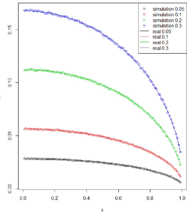
Theorem 1The mean edge density of an AR(1) recurrence network is equal to 2 N(N −1) N X i=1 N−i X h=1 2Φ( s 1−φ2 2−2φh)−1 ! . (4.14)
Proof: By lemma 1, it is easy to calculate the mean edge density of an ARMA (p,q) model:
E(ˆρ(ε)) =E( 1 N(N −1) N X i,j=1 Yi,j(ε)) =E( 2 N(N −1) N X i=1 N X j=i+1 Yi,j(ε)) =E( 2 N(N −1) N X i=1 N−i X h=1 Yi,i+h(ε)) = 2 N(N −1) N X i=1 N−i X h=1 2Φ( Ch )−1
For an AR(1) model,
Ch2 = h−1 X j=0 φ2j + ∞ X k=0 (φk+h−φk)2 = h−1 X j=0 φ2j + (φh−1)2 ∞ X k=0 φ2k = 1−φ 2h 1−φ2 + (φ h−1)2 1 1−φ2 = 2−2φ h 1−φ2 Thus E(ˆρ(ε)) = 2 N(N −1) N X i=1 N−i X h=1 2Φ( s 1−φ2 2−2φh)−1 ! .
The mean edge density can be interpreted as the probability of recurrence in the network. Figure3shows the simulation results and real mean edge density curves given by Theorem 1. The simulated mean edge densities are calculated based on 100 sequences for each AR (1) coefficients from 0.01 to 0.99 and for = 0.05, 0.1, 0.2, 0.3. It is easy to see that the higher AR(1) coefficients the lower edge density, and the higher threshold distance the higher edge density.
Figure 3: Four points lines: Simulation results of mean edge density for = 0.05, 0.1, 0.2, 0.3; Four solid lines: The real mean edge density for= 0.05, 0.1, 0.2, 0.3
4.4 SIMULATION STUDY
In this section, we conduct a simulation study to evaluate the performance of our proposed sequen-tial clustering method and compare it with some other common sequensequen-tial clustering methods. The dynamical system we check is logistic map:
xn+1 =rxn(1−xn),
where r is the parameter. The logistic map is a polynomial mapping with degree 2. It is often used as an archetypal example of how chaotic and complicated behavior could arise from simple nonlinear dynamical systems. The range of interest for parameterr is [0, 4]. Depending on the different values ofr, the behaviors of the sequence can be completely different. For example, ifr
is between [2, 3], the sequence would eventually converge to the same value r−r1, independent of the initial conditions; ifris greater than 3.56995, the system exhibits chaotic behavior.
We repeat the parameter setting inMarwan et al. (2009). Two groups of sequences are simu-lated, one with r = 3.83, another with r = 3.679. The former type is called period-3 dynamics while the latter one is called band merging. Each sequence has random initial state that follows a uniform (0,1) distribution. We tried two different settings of random noise: uniform(-0.1, 0.1) and uniform (-0.2, 0.2). Each group contains 20 sequences and the length of each sequence is T=500, 800 or 1000.
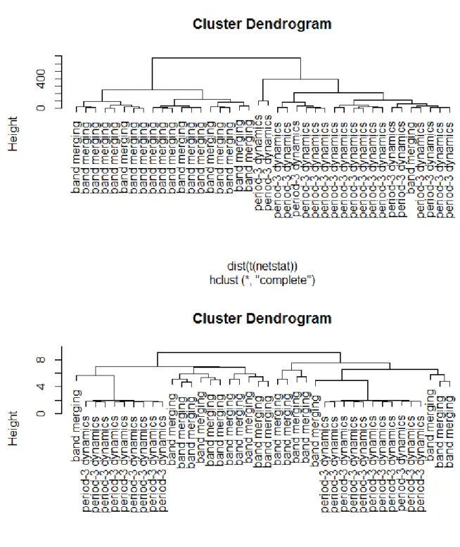
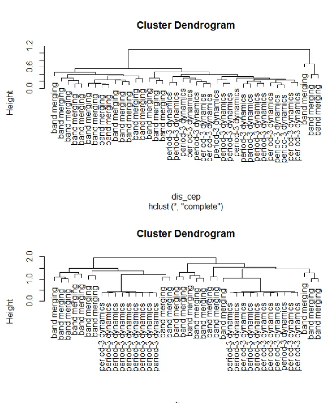
When doing clustering, we letε = 0.0015for uniform (-0.1, 0.1) noise and letε = 0.0025for uniform (-0.2, 0.2) noise, which makes mean edge density less than 1%. The ERGM terms used are mean degree, number of two-paths, degree distribution for 1 to 4 for T=500, 800 and degree distribution for 2 to 5 for T=1000 . Figure4shows the dendrogram of RN-ERGM clustering and dendrogram of raw data with Euclidean distance when T=500 and noise is Uniform(-0.1, 0.1). Figure5shows the dendrogram of LPC cepstral coefficients clustering (Kalpakis et al.,2001) and dendrogram of correlation based clustering method proposed byGolay et al.(1998). All methods use hierarchical clustering with complete linkage. We repeat the simulation with same setting 50 times. The average performance is reported in Table1, Table2, Table3, Table 4. In general, our proposed method performs pretty well. In particular, when the length of sequence increases, the
proposed method performs better. By increasing the value ofε, our method filters out some larger noises.
Table 1: Accuracy rates of different methods, using U(-0.1,0.1) noise
U(-0.1,0.1) raw RN-ERGM AR.LPC.CEPS COR
T=500 0.6000 0.8650 0.6512 0.5925
T=800 0.5775 0.8750 0.8550 0.5612
T=1000 0.5538 0.9850 0.9175 0.5662
Table 2: Adjusted Rand Index of different methods, using U(-0.1,0.1) noise
U(-0.1,0.1) raw RN-ERGM AR.LPC.CEPS COR
T=500 0.0465 0.5401 0.2367 0.0384
T=800 0.0081 0.6814 0.6786 -0.0008
T=1000 -0.0021 0.9478 0.8060 0.0058
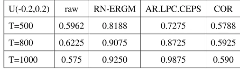
Table 3: Accuracy rates of different methods, using U(-0.2,0.2) noise
U(-0.2,0.2) raw RN-ERGM AR.LPC.CEPS COR
T=500 0.5962 0.8188 0.7275 0.5788
T=800 0.6225 0.9075 0.8725 0.5925
T=1000 0.575 0.9250 0.9875 0.590
Table 4: Adjusted Rand Index of different methods, using U(-0.2,0.2) noise
U(-0.2,0.2) raw RN-ERGM AR.LPC.CEPS COR
T=500 0.0319 0.4302 0.3226 0.0202
T=800 0.0633 0.6852 0.6629 0.0354
4.5 APPLICATION
4.5.1 Case Study: Measles Patterns in the United States
In addition to our simulation study, we will use our proposed method on a real-world data set from epidemiology. Disease control is typically organized by administrative area, but this is not how disease transmission works. Therefore, it is a worthy effort to try to cluster geographical units (U.S. states) into areas that have similar measles transmission patterns. Cummings et al.(2006) used hierarchical clustering on the raw measles sequences of provinces in Cameroon. However, doing hierarchical clustering directly on the raw data neither explains the whole story well in theory nor performs well in practice. Therefore, new works that have more solid theoretical foundation and better practical performance would be meaningful.
Nonlinear dynamics of infectious diseases provide a clear illustration of the essentially spatio-temporal nature of population dynamics. The paradigm is provided by the oscillatory dynamics of acute, immunizing infections such as measles. Many researchers have discussed the problems from perspective of nonlinear dynamics (Bartlett, 1956), (Finkenst¨adt and Grenfell, 2000), (Grenfell et al., 2002), (Xia et al., 2004). Those works indicate the potential of using nonlinear dynamics approaches. The availableProject Tychodata provides weekly measles surveillance data at both city and state level of the pre-vaccine era in the US. We use state level measles time series between 1940 and 1954, during which time period we have fewer missing values.
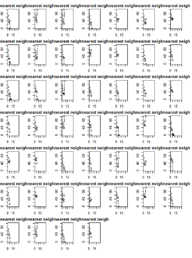
We removed the sequences that contain more than20% missing values. For the remaining 46 sequences, linear interpolation was used for missing values. All sequences were log transformed and normalized. Nonlinear surrogate testing were done for all sequences to verify the nonlinear dynamics and 36 of them were significant. Through previous study and the testing results, our RN-ERGM clustering approach has potential to work well for the given data set. Figure6shows the changes of mutual information with differentτof all 46 sequences. Most of the sequences get a minimum atτ = 14orτ = 15. Next we consider the embedding dimensionm. Figure7shows that all FNNs decrease quickly. Since this approach usually would overestimate embedding dimension, we would use smaller one,m= 3orm = 4. The threshold distanceεneeds to be confirmed with ERGM terms and other two embedding parameters. The rule of thumb is to choose aεthat makes
the edge density less than1%, makes the network can be represented by lower centrality degree and makes ERGMs converge. A grid search was done to find three parameters and ERGM terms. Our final model setτ = 14,m = 3,ε = 0.25with one to four centrality degree, edge density and two-path as model terms.
Figure8shows the gap statistic. It appears that there is a local peak whenk = 5. We used this as a reference to set our cluster size equal to 5. Figure9, Figure10, Figure11and Figure12show the clustering results using our RN-ERGM approach, dynamic time warping distance, Maharaj and Piccolo model-based dissimilarity respectively. The last two clustering approaches are based on the ARIMA models. For comparison, we used the hierarchical clustering with five clusters in all approaches. It is easy to see that the distribution of measles pattern clusters matches better with geographical distribution in our approach than other three approaches. In fact, the clusters of measles pattern are highly correlated with their longitude.
Table 5shows Silhouette coefficients for our methods and some other methods. The results show that our proposed method performs better than some other sequential clustering methods.
4.5.2 UCR Time Series Data
UCR Time Series Classification Archive Chen et al. (2015) is a prominent public database for time series classification. Although the database is initially built for comparison of classification methods, we could still utilize it to compare different clustering methods. One disadvantage of this public database is that it does not show how those data sets are collected and their original meanings. But the good part is that all sequences of all data sets here are labeled. We can use adjusted Rand index, mutual information and accuracy rate to compare performance of our method with some other methods.
Dynamic Time Warping (DTW) clustering is one of the most popular clustering methods in the field of time series clustering. It has shown that it is powerful and robust in many applications and case studies. We apply a raw Euclidean distance based hierarchical clustering method, DTW clustering and our proposed method on five public data sets. The first method above is regarded as a baseline method. We focus on the performance of our proposed RN-ERGM method and DTW clustering.
Figure 9: Map of clustering by RN-ERGM approach
Figure 11: Map of clustering by Maharaj model-based Dissimilarity
Table 5: Performance comparison of different methods silhouette l2 0.09324 dtw 0.0616 Piccolo 0.0650 Cepstral 0.0697 Maharaj 0.2002 ERGM 0.2298
Table6, Table7, Table8, Table9and Table10show the results. For FaceFour and CinC ECG data, we just calculate adjusted Rand index and mutual information since they have more than two unique labels for which accuracy loses the meaning. The results shows that our proposed method performs better in all five data sets.
Table 6: Performance evaluation on Coffee Data
Coffee Accuracy Adjusted Rand Index Mutual Information
l2 0.5714 0.0158 0.0407
dtw 0.8036 0.3578 0.2418
Table 7: Performance evaluation on Gun Point Data
Gun Point Accuracy Adjusted Rand Index Mutual Information
l2 0.5400 0.0056 0.0286
dtw 0.5800 0.0242 0.0589
ERGM 0.8100 0.3816 0.2499
Table 8: Performance evaluation on Wafer Data
Wafer Point Accuracy Adjusted Rand Index Mutual Information
l2 0.6540 -0.005 0.001
dtw 0.8520 0.0331 0.001
ERGM 0.8290 0.1035 0.007
Table 9: Performance evaluation on FaceFour Data
FaceFour Adjusted Rand Index Mutual Information
l2 -0.1031 0.0562
dtw -0.0974 0.0614
ERGM 0.1067 0.0297
Table 10: Performance evaluation on CinC ECG Data
CinC ECG Adjusted Rand Index Mutual Information
l2 0.65 0.0122
dtw 0.625 0.0018
5.0 HOW MUCH INFORMATION IS CONTAINED IN A RECURRENCE NETWORK?
5.1 MOTIVATION
One important assumption that our RN-ERGM clustering algorithm would work is that the re-currence networks must contain enough information of the original time series. Besides those clustering performance metrics that we have used to show the effectiveness of our algorithm, we would like to use another task, classification, and tools from another field, image recognition, to further study the properties of recurrence networks.
As illustrated in Chapter 2, we call weighted recurrence networks as recurrence images. Since our time series have been converted to “virtual images”, many advanced image recognition algo-rithms may work here. We would introduce one of the most popular class of models in machine learning and artificial intelligence communities, convolutional neural network (CNN) in next sec-tion. We believe that if recurrence images can be classified well by CNN on public time series database, they contain more than enough information of the original time series. The method proposed in this chapter is also self-contained for time series classification tasks.
5.2 INTRODUCTION
In recent years, Convolutional Neural Networks (CNN), as one of the core class of models in deep learning, has shown huge successes in many fields, such as speech recognition, natural lan-guage processing, information retrieval and especially for computer vision. It has many famous applications, such as self-driving cars, photo search, face recognition, artificial robot and online recommender systems. Roughly speaking, a CNN architecture is formed by a stack of selective
and distinct layers that transform the input volume into an output volume via linear combinations of input volume and differentiable activation functions.
One of the key feature of CNN is that it can automatically learn complex feature representations for you. This saves people much time compared with traditionally manual data cleaning and feature engineering procedures which usually take around 80% of time of data scientists. In addition, CNN outperforms other traditional machine learning algorithms with huge margins in all famous computer vision competitions since 2012.
The pioneering CNN architecture, LeNet, was developed by LeCun et al. (1998) in 1998. However The ability to process higher resolution images needs larger and more convolutional layers in the architecture. The availability of computing resources constrained the performance of CNN. CNN did not receive enough attention until 2012. The milestone work, commonly known as AlexNet, by Krizhevsky et al. (2012) is widely regarded as one of the most influential CNN architecture in the field. It was submitted to the ImageNet ILSVRC challenge in 2012 and achieved a top-5 test error rate of 15.3%, compared to 26.2% achieved by the second-best entry which used traditional computer vision algorithms. Their work popularized CNN in computer vision.
After AlexNet, the winner of ILSVRC 2013, ZF Net byZeiler and Fergus(2014), the winner of ILSVRC 2014, GoogLeNet bySzegedy et al.(2015) and the runner-up of ILSVRC 2014, VGGNet by Simonyan and Zisserman (2014) are some phenomenon work in the field. They significantly increase the classification accuracy each year on ImageNet. Perhaps one of the most important thought from these papers is that deeper neural networks are more efficient than wider neural networks given the fixed model complexity. The pretrained models from those architectures can be further fine-tuned on other image data sets and show good generalization performance.
Another very influential work is ResNet, the winner of ILSVRC 2015, by He et al. (2016a),
He et al.(2016b) from Microsoft Research Asia. ResNet has a very deep, 152-layer, architecture and sets new records in many ILSVRC challenges. Their best result based on ensembles has an incredible top-5 error rate of 3.6% compared with human benchmark of 5.1% error rates. After ResNet, the progress in ImageNet classification is slow down since people are closer and closer to the Bayes error.
In this thesis, we propose a method to classify time series data based on CNN models. We intend to connect time series analysis with image processing via weighted recurrence networks
generated from the original time series. More specifically, each weighted recurrence network is processed as a recurrence image. We then build CNN models to process and classify recurrence images as common image classification problems. We consider two types of CNN architectures, one VGGNet style plain networks, one ResNet style residual networks.
5.3 RELATED WORK
Time series classification has been studied for a long time. Most of the traditional algorithms we mentioned in Chapter 2 for time series clustering can be easily converted to corresponding clas-sification algorithms. For algorithms that define pairwise similarity or distance metrics between the time series directly, a k-Nearest Neighbor (kNN) classifier can be built on top of those metrics. For algorithms that extract dense feature vectors from the original time series, a traditional classi-fication algorithm, such as random forest or support vector machine can be used on top of those feature vectors.
There are several studies that share some common elements of our method. Silva et al.(2013) measured the similarity between time series via recurrence plots using a Kolmogorov complexity based distance, Campana-Keogh (CK-1) distance. They used Recurrence Patterns Compression Distance (RPCD) to refer to the CK-1 distance over recurrence plots. Michael et al.(2015) intro-duced another distance measure between time series based on the compression of cross recurrence plots (CRPCD). Both methods used kNN to classify time series based on the pairwise distance matrix. Souza et al. (2014) proposed a method that extracts time series features from RP manu-ally, and used those features to classify time series data with support vector machine (SVM).Dalto
(2014) built CNN with variables that were processed via an input variable selection (IVS) algo-rithm. Cui et al.(2016) proposed a Multi-scale Convolutional Neural Network (MCNN), which incorporates feature extraction and classification in a single framework. MCNN can automatically extract features at different scales and frequencies.
Some of the methods above use the information extracted from the RPs and build classifiers using traditional classification algorithms. Some others extract the information from the raw time series and build CNNs on top of them. However, none of the methods above give simple solutions
and connect raw time series, recurrence images and most advanced CNN models together as our method. We will show comparison of our method with some of these methods in later sections.
5.4 PROPOSED METHOD
The steps of our proposed recurrence images based convolutional neural network (RI-CNN) clas-sification method is summarized below:
(1) Construct recurrence images for all sequences. Embedding parametersm, time delay parame-terτ are considered as the hyperparameters of the models.
(2) Preprocess recurrence images with image scaling, data augmentation or both of above to avoid overfitting.
(3) Consider two CNN architectures, one with VGGNet style, one with ResNet style. The final model with all hyperparameters is selected based on the prediction performance on the valida-tion set.
We will show the details and reasoning of each step in following.
5.4.1 Recurrence Images and Why CNN Works A recurrence image is defined as:
Ri,j(ε) = ||si−sj|| (5.1)
where|| · || is a suitable norm (usually the Euclidean norm) in the considered phase space, si =
(ui, ui+τ, ..., ui+(m−1)τ)T is the reconstructed phase space vector observed at timeifor the trajec-torys(t), ui is the original scalar time series,m is the embedding dimension,τ is the time delay parameter.
In a traditional fully connected neural network, each neuron in a hidden layer would connect all neurons of the previous layer. If layerl+ 1hasnneurons andlhasmneurons, we would have
n×mparameters. For common tabular data, this might not be a big issue. However, the number of parameters would be huge for image data. Suppose the input data(layer) is a32×32×3image. If
we set 100 neurons in the first hidden layer, we would have32×32×3×100 = 307200parameters for just a single layer. Obviously, the huge number of parameters would quickly lead to overfitting.
The CNN could solve this issue based on two important assumptions for input image data:
(1) Local Connectivity: Each neuron is only connected to a local region of the input volume. This works since common image data are full of local structures. For example, we do not need to check all pixels to recognize a bird’s beak. A few pixels in general is enough.
(2) Parameter Sharing for each filter: Each filter is like a detector that would scan the whole image map to detect a single local structure/feature. To detect different features, we just add more filters in the network and let the algorithm learn the weights automatically. Parameter sharing means that all neurons correspond to same filter would have the same weights. This works since for most of computer vision tasks a bird’s beak appears at the top-left corner is same as it appears at bottom-right corner, i,e., translationally-invariance.
It is straightforward to see that recurrence images satisfy those two assumptions as common images. Since recurrence images are just weighted version of recurrence plots, we will just discuss recurrence plots for symbol simplicity.
First, recurrence plots have many local structures. For example, a diagonal lineRi+k,j+k = 1 for (k = 1...l, where l is the length of the diagonal line) when the trajectory revisits the same region of the phase space at different times. The CNNs can capture those local structures easily. Second, in most of cases we just care about the number of occurrences of some local patterns when doing recurrence quantification analysis. That means if a diagonal line is useful to compute at some spatial position (x1, y1, then it should also be useful to compute at a different position
(x2, y2. Thus recurrence images satisfy the two assumptions above.
5.4.2 Image Scaling and Data Augmentation
Although using CNN instead fully connected networks has already reduced the model complexity a lot, the total number of parameters is still too much for recurrence images. In fact, real world time series can be very long. However for common image data, the resolution of the image usually has an upper limit. Thus, we need to scale our recurrence images to the appropriate size. More specifically, we need to downsample the original higher resolution recurrence images to smaller
images. This can be done in several ways in computer vision and the discussion of those algorithms is beyond the scope of this thesis. Here we use a bilinear interpolation algorithm, one of the most common algorithms in the field. The dimension of the scaled recurrence images would be considered as a hyperparameter which would be tuned based on validation set.
For some time series datasets, the length of time series is quite small but we do not have a large enough training set. We can consider the crop a number of patches from a recurrence image uniformly from top-left to bottom-right. The crop size is a hyperparameter that can be tuned using validation set.
The process is as follows: At training step, first crop k patches from each recurrence image. Then just consider each patch as a training data point. That is:
(Xi, yi)−→(Xi(1), yi), ...(Xi(k), yi),
where Xi is the matrix of a recurrence image in the training set, yi is the label of original time series,Xi(j)forj = 1, .., kiskpatches of imagei.
At testing step, first still crop k patches from each recurrence image. Then use our trained CNN model to make predictions on all patches and get the mean of softmax layer output(a multinomial probability vector) of all the patches that are cropped from the same image. We could then predict based on the aggregate probability vectors. That is:
Xi −→Xi(1), ...Xi(k) −→pi(1), ...pi(k) −→
X
k
pi(k) −→yˆi.
Sometimes, we may have limited training samples while each time series is quite long. We can then consider using both image scaling for dimension reduction and data augmentation for increasing size of training set. The exact strategy is data driven and tuned based on validation set.