Accelerating data-intensive scientific visualization and computing through parallelization

(1)

New Jersey Institute of Technology

Digital Commons @ NJIT

Dissertations Theses and Dissertations

Summer 2016

Accelerating data-intensive scientific visualization

and computing through parallelization

Dongliang Chu

New Jersey Institute of Technology

Follow this and additional works at:https://digitalcommons.njit.edu/dissertations Part of theComputer Sciences Commons

This Dissertation is brought to you for free and open access by the Theses and Dissertations at Digital Commons @ NJIT. It has been accepted for inclusion in Dissertations by an authorized administrator of Digital Commons @ NJIT. For more information, please contact

[email protected].

Recommended Citation

Chu, Dongliang, "Accelerating data-intensive scientific visualization and computing through parallelization" (2016).Dissertations. 94.

(2)

Copyright Warning & Restrictions

The copyright law of the United States (Title 17, United

States Code) governs the making of photocopies or other

reproductions of copyrighted material.

Under certain conditions specified in the law, libraries and

archives are authorized to furnish a photocopy or other

reproduction. One of these specified conditions is that the

photocopy or reproduction is not to be “used for any

purpose other than private study, scholarship, or research.”

If a, user makes a request for, or later uses, a photocopy or

reproduction for purposes in excess of “fair use” that user

may be liable for copyright infringement,

This institution reserves the right to refuse to accept a

copying order if, in its judgment, fulfillment of the order

would involve violation of copyright law.

Please Note: The author retains the copyright while the

New Jersey Institute of Technology reserves the right to

distribute this thesis or dissertation

Printing note: If you do not wish to print this page, then select

“Pages from: first page # to: last page #” on the print dialog screen

(3)

The Van Houten library has removed some of the

personal information and all signatures from the

approval page and biographical sketches of theses

and dissertations in order to protect the identity of

NJIT graduates and faculty.

(4)

ABSTRACT

ACCELERATING DATA-INTENSIVE SCIENTIFIC VISUALIZATION AND COMPUTING THROUGH PARALLELIZATION

by

Dongliang Chu

Many extreme-scale scientific applications generate colossal amounts of data that require an increasing number of processors for parallel processing. The research in this dissertation is focused on optimizing the performance of data-intensive parallel scientific visualization and computing.

In parallel scientific visualization, there exist three well-known parallel archi-tectures, i.e., sort-first/middle/last. The research in this dissertation studies the composition stage of the sort-last architecture for scientific visualization and proposes a generalized method, namely, Grouping More and Pairing Less (GMPL), for order-independent image composition workflow scheduling in sort-last parallel rendering. The technical merits of GMPL are two-fold: i) it takes a prime factorization-based approach for processor grouping, which not only obviates the common restriction in existing methods on the total number of processors to fully utilize computing resources, but also breaks down processors to the lowest level with a minimum number of peers in each group to achieve high concurrency and save communication cost; ii) within each group, it employs an improved direct send method to narrow down each processor’s pairing scope to further reduce communication overhead and increase composition efficiency. The performance superiority of GMPL over existing methods is evaluated through rigorous theoretical analysis and further verified by extensive experimental results on a high-performance visualization cluster.

The research in this dissertation also parallelizes the over operator, which is commonly used for α-blending in various visualization techniques. Compared with its predecessor, the fully generalized over operator is n-operator compatible.

(5)

To demonstrate the advantages of the proposed operator, the proposed operator is applied to the asynchronous and order-dependent image composition problem in parallel visualization.

In addition, the dissertation research also proposes a very-high-speed pipeline-based architecture for parallel sort-last visualization of big data by developing and integrating three component techniques: i) a fully parallelized per-ray integration method that significantly reduces the number of iterations required for image rendering; ii) a real-time over operator that not only eliminates the restriction of pre-sorting and order-dependency, but also facilitates a high degree of parallelization for image composition.

In parallel scientific computing, the research goal is to optimize QR decom-position, which is one primary algebraic decomposition procedure and plays an important role in scientific computing. QR decomposition produces orthogonal bases, i.e.,“core” bases for a given matrix, and oftentimes can be leveraged to build a complete solution to many fundamental scientific computing problems including Least Squares Problem, Linear Equations Problem, Eigenvalue Problem. A new matrix decomposition method is proposed to improve time efficiency of parallel computing and provide a rigorous proof of its numerical stability.

The proposed solutions demonstrate significant performance improvement over existing methods for data-intensive parallel scientific visualization and computing. Considering the ever-increasing data volume in various science domains, the research in this dissertation have a great impact on the success of next-generation large-scale scientific applications.

(6)

by

Dongliang Chu

A Dissertation

Submitted to the Faculty of New Jersey Institute of Technology

in Partial Fulfillment of the Requirements for the Degree of Doctor of Philosophy in Computer Sciences

Department of Computer Science August 2016

(7)

(8)

APPROVAL PAGE

Dongliang Chu

Dr. Chase Wu, Dissertation Advisor Date

Associate Professor of Computer Science, New Jersey Institute of Technology

Dr. Cristian M. Borcea, Committee Member Date

Associate Professor of Computer Science, New Jersey Institute of Technology

Dr. Alexandros Gerbessiotis, Committee Member Date Associate Professor of Computer Science, New Jersey Institute of Technology

Dr. Xiaoning Ding, Committee Member Date

Assistant Professor of Computer Science, New Jersey Institute of Technology

Dr. Yi Chen, Committee Member Date

(9)

BIOGRAPHICAL SKETCH

Author: Dongliang Chu

Degree: Doctor of Philosophy

Date: August 2016

Undergraduate and Graduate Education:

• Doctor of Philosophy in Computer Science

New Jersey Institute of Technology, Newark, NJ, 2016 • Master of Science in Computer Engineering

Zhengzhou University, Zhengzhou, Henan, 2012 • Bachelor of Science in Mathematics

North China University of Water Resources and Electric Power (NCWU), Zhengzhou, Henan, 2009

Major: Computer Science

Presentations and Publications:

D. Chu, C. Q. Wu, J. Gao, L. Wang. On a Generalized Scheme for Order-Independent Image Composition in Parallel Visualization. International Performance Computing and Communications Conference 2013.

D. Chu, C. Q. Wu, Z. Wang, Y. Wang. A Fully Generalized over Operator with

Applications to Image Composition in Parallel Visualization for Big Data Science. International Conference on Parallel and Distributed Systems 2014. D. Chu, C. Q. Wu.On a Pipeline-based Architecture for Parallel Volume Visualization

of Big Data. International Conference for Parallel Processing 2016.

D. Chu, C. Q. Wu. The Order-dependence eliminated and efficiency optimized

parallel over Operator. In preparation for Journal of Parallel and Distributed

Computing.

D. Chu, C. Q. Wu. V4BD: A Very High-speed Value-added Volume Visualization Architecture. In preparation for Transactions on Visualization and Computer Graphics.

(10)

Dedicated to my beloved parents: (谨此献给我挚爱的双亲:) Faying Chu(褚发营)，father(父亲) Lamei Shen(沈腊_梅)，mother(母亲)

“No pain, No gain” “梅花香自苦寒来”

(11)

ACKNOWLEDGMENT

Longing and longing, waiting and waiting, finally it comes to the conclusion of my Ph.D. student life, which is definitely impossible without appearances of so many amazing features in my life.

The top-ranked and valued-most character is my advisor, Dr. Chase Q. Wu. There is so much appreciation I want to convey such that I can’t figure out which is the most suitable for expressing here. I will just enumerate a few that are most fresh in my mind currently. Honestly speaking, without Dr. Wu, I would have had no opportunity to conduct or start Ph.D. study in U.S.. He guided my entire process of application, first entry into the U.S., settlement at a totally strange location, etc. As I soundly got into the role of a Ph.D. student under his advisement, it constantly made me feel lucky and grateful for the precious opportunity that I was granted. He always patiently helped me formulate the research problem, discussed the possible solutions and polished the according draft again and again. I was improved and benefitted from this significantly. Of course, there are other forms of help that I want to share. However, I have to stop here and keep all of them in my heart forever.

Committee members of my Ph.D. dissertation instructed and benefited my Ph.D. a lot as well. Each of them devoted significant amounts of time to my dissertation, provided huge amounts of valued comments, and always kept me on the right track. I want to express sincere appreciation to Dr. Cristian M. Borcea, Dr. Alexandros Gerbessiotis, Dr. Xiaoning Ding, and Dr. Yi Chen.

I also want to express hearted thanks to the considerable help that I received from the department of Graduate Studies. Special thanks to Dr. Sotirios G. Ziavras, Ms. Clarisa Gonz´alez-Lenahan, Ms. Lillian Quiles and Mr. David Tress, Dr. George Olsen, Dr. Ali Mili, Ms. Angel Butler, .

(12)

TABLE OF CONTENTS

Chapter Page

1 INTRODUCTION . . . 1

1.1 Parallel Scientific Visualization and Image Composition . . . 1

1.2 Parallel Scientific Computing and QR Decomposition . . . 2

2 IMAGE COMPOSITION OPERATOR . . . 4

2.1 overComposition Operator . . . 4

2.2 A Fully Generalizedover Image Composition Operator . . . 6

2.2.1 Extension from Two Operands to Multiple Ones . . . 6

2.2.2 An In-depth Illustration of the New over Operator . . . 9

2.3 Asynchronous, Order-known Image Composition . . . 13

2.3.1 Algorithm Design, Analysis, and Optimization . . . 14

2.3.2 Theoretical Performance Analysis . . . 16

2.3.3 Implementation and Experimental Results . . . 27

2.4 Asynchronous, Order-unknown Image Composition . . . 32

2.4.1 Algorithm Design and Analysis . . . 33

2.4.2 SGOUC . . . 33

2.4.3 PGOUC . . . 35

2.4.4 Theoretical Performance Analysis . . . 36

2.5 The In-practice Real-timeover Operator . . . 45

2.5.1 IROO Based Image Composition and the General Optimization Strategies . . . 45

2.5.2 IROO Based Image Composition Algorithms . . . 48

2.5.3 AM . . . 51

2.5.4 DM . . . 53

(13)

TABLE OF CONTENTS (Continued)

Chapter Page

3.1 Image Composition Workflow Organization . . . 62

3.2 GMPL Algorithm for Image Composition Workflow Scheduling . . . 64

3.2.1 Algorithm Design . . . 64

3.2.2 Algorithm Analysis . . . 69

3.2.3 Theoretical Analysis and Comparison of Latency Performance 74 3.2.4 Performance Evaluation . . . 82

4 V4BD . . . 85

4.1 Background . . . 85

4.2 Related Work . . . 87

4.2.1 Raycasting and its Acceleration . . . 87

4.2.2 over Operator for Image Composition . . . 87

4.2.3 Sort-last Visualization Architecture . . . 88

4.3 V4BD: A Very High-speed Value-added Volume Visualization Architecture for Big Data. . . 88

4.3.1 Parallelized Per-Ray Integration (PPRI) . . . 91

4.3.2 Real-Time over Operator for Online Image Composition . . . 92

4.3.3 A Tile-based Visualization Pipeline . . . 95

5 QR DECOMPOSITION . . . 108

5.0.5 Existing Mainstream Sequential QR Decomposition Methods . 108 5.1 Parallelization for QR Decomposition . . . 113

5.1.1 Requisite Components in Parallel QR Factorization . . . 113

5.1.2 Parallelized QR Decomposition Methods and Their Performances115 5.2 Supportive Theorems for Parallel QR Decomposition . . . 115

(14)

TABLE OF CONTENTS (Continued)

Chapter Page

6.1 Image Composition in Scientific Visualization . . . 123 6.2 QR Decomposition in Scientific Computing . . . 124 BIBLIOGRAPHY . . . 125

(15)

LIST OF TABLES

Table Page

3.1 Latency Performance Analysis of Four Methods in Comparison, where Tl is the Connection Establishing Time, Tc is the Image Transfer Time,Tb is the Image Blending Time . . . 80 5.1 Stability Analysis of Four Methods in Comparison . . . 112 5.2 Latency Performance Analysis of Four Methods in Comparison[15] . . . 116

(16)

LIST OF FIGURES

Figure Page

2.1 A general illustration of dividing the pixel area by n geometries. . . 10

2.2 A specific illustration of dividing the pixel area by 3 geometries. . . 12

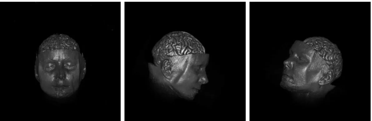
2.3 Composited images of Human Brain. . . 28

2.4 Composited images of HIPIP Surfaces. . . 28

2.5 Composited images of Jet Ejections. . . 29

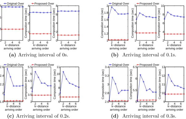
2.6 Comparison of twooveroperators using images of size 20482_{: composition} time versus arriving order. The three sub-figures in Figures 2.6a, 2.6b, 2.6c, and 2.6d correspond to the cases of 8, 16, 32 input images, respectively, from left to right. . . 30

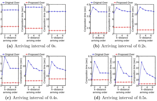
2.7 Comparison of two operators using images of size 30722_{: composition time} versus arriving order. The three sub-figures in Figure 2.7a, 2.7b, 2.7c, and 2.7d correspond to the cases of 8, 16, and 32 input images, respectively, from left to right. . . 31

2.8 The P Pack{} data structure for sequential image composition based on the proposed operator. . . 33

2.9 The ParaP Pack{} data structure for parallelized image composition based on the proposed operator. . . 35

2.10 Comparisons between SGOUC and PGOUC. . . 37

2.11 Composited images of Human Brain. . . 41

2.12 Composited images of HIPIP Surfaces. . . 41

2.13 Composited images of Jet Ejections. . . 41

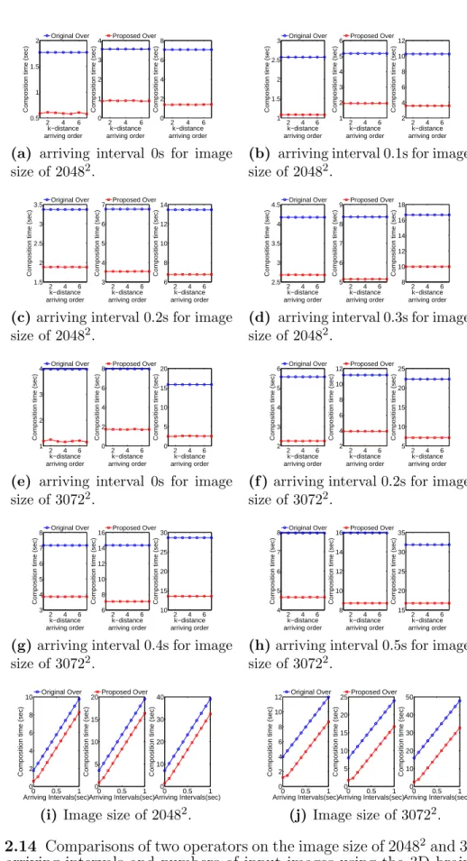
2.14 Comparisons of two operators on the image size of 20482 and 30722 with varying arriving intervals and numbers of input images using the 3D brain dataset. The three subfigures in each group correspond to the cases of 8, 16, and 32 input images, respectively, from left to right. . 44

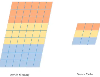
2.15 Illustration for the correlation between the global memory and high-speed cache. . . 50

2.16 Illustrating figure for each thread’s assignment of pixel positions. . . 52

2.17 Illustration for the correlation between the global memory and high-speed cache. . . 53

(17)

LIST OF FIGURES (Continued)

Figure Page

2.18 Illustration of the assignment of images to streams. . . 54 3.1 Illustration of the proposed GMPL method in the case of 10 processors. 70 3.2 Latency performance of different methods on different image sizes and

numbers of processors. . . 83 3.3 Composited brain images of size 20482 _{using the GMPL method.} _{. . . .} ₈₄ 4.1 The execution process of the proposed V4BD architecture in a simple case

of three rendering/composition units. . . 89 4.2 Illustration of the proposed parallel ⊕ operation for per-ray integration

with 8 sampling points. . . 93

4.3 The F ragCompInf o{} data structure for storing the composition

infor-mation of each fragment. . . 94 4.4 An illustration of the pipeline in [11] (left) and the proposed one (right),

where “RS” represents a rendering step, “TS1” represents a data transfer from a rendering unit to a composition unit, “CS” represents a composition step, “TS2” represents a data transfer from a composition unit to a display unit, and “DS” represents a display step. . . 96 4.5 Composited images of Human Brain, HIPIP and Jet Ejection. . . 101 4.6 Performance comparison between the proposed and existing raycasting

methods. . . 102 4.7 Comparisons of twooveroperators on the image size of 20482 _{in subfigures}

(a,b,c,d) and 30722 in subfigures (e,f,g,h) using the 3D brain dataset with varying arriving intervals and numbers of input images. The three figures in each subfigure correspond to the cases of 8, 16, and 32 input images, respectively, from left to right. . . 105 4.8 Comparisons of twooveroperators on the image size of 20482 in subfigure

(a) and 30722 _{in subfigure (b) using the 3D brain dataset with varying} arriving intervals and numbers of input images arriving in an “ideal” order. The three figures in subfigures (a) and (b) correspond to the cases of 8, 16, and 32 input images, respectively, from left to right. . 106

(18)

LIST OF FIGURES (Continued)

Figure Page

4.9 Comparison of the proposed and existing visualization pipeline with 8, 16, and 32 rendering/composition nodes, where “Traditional” represents the traditional sort-last pipeline, “Pipeline+over” represents the tile-based pipelining structure using only the proposed over operator, and “V4BD” represents the tile-based pipelining structure using the proposed rendering and composition methods. . . 107 5.1 Commonly-used parallel processor architecture. . . 114 5.2 Performances of different algorithms on different sizes of data. . . 122

(19)

CHAPTER 1 INTRODUCTION

The scale of data generated by modern scientific applications is rapidly increasing, ranging from terabyes at present to petabytes or exabytes down the road in the predictable future. Such data, now commonly termed as “big data”, can be resulted from various sources including simulations, experiments, or observations, and must be processed and analyzed in a timely manner for scientific exploration and knowledge discovery. Among many existing methods for data processing/analytics, scientific visualization and computing have been well recognized and widely used in broad science communities to make sense of the data. However, the sheer volume of today’s scientific data has posed a daunting challenge on traditional visualization and computing technologies. Parallel scientific visualization and computing have proven to be promising solutions to handle data of such scales.

1.1 Parallel Scientific Visualization and Image Composition

Many parallel visualization architectures have emerged in the last decade [48, 49, 30, 43, 1, 60]. As put forth by Molnar et al., according to the time when primitives

in the raw data are sorted on their corresponding processors, parallel visualization architectures can be classified into three categories, i.e., sort-first, sort-middle, and sort-last [47]. Although the instances in each category may differ in their particular implementations, they generally share some common features. In sort-first, each primitive in the raw data is assigned to a certain processor, which is responsible for a predivided region of the display screen. This scheme could save network communications between the processors due to the predetermined locality of each primitive, but may result in unbalanced workload among the processors due to the static screen partitioning. In sort-last, s are not assigned as strictly. Instead, they

(20)

are rendered into pixels by the processors they are initially assigned to, and these distributed pixels must be composited into a final image. This scheme may achieve a high level of workload balance at the cost of increased network communications. In sort-middle, the entire visualization process is naturally divided into two distinctive stages: geometry processing and rasterization. Such a partitioning of visualization groups together the operations with similar purposes and distinguishes from others. This scheme may consume more bandwidth and incur a longer processing time, and hence is investigated in more theoretical than practical settings.

Among the above three well-known parallel architectures, sort-last is often preferred in many applications due to its adaptability to load balancing. In general, the sort-last architecture comprises of two stages: rendering and composition [67]. We mainly focus on composition stage here, which encompasses huge number of research topics that are of practical importance while still not satisfactorily resolved in times of “Big Data”, including the composition operator, the communication overheads among participating computing units and so on.

1.2 Parallel Scientific Computing and QR Decomposition

QR decomposition is a long existing and widely used algebraic decomposition procedure in scientific computing. Given a non-singular matrix An×n, its QR decomposition is defined as

A=Q·R,

where Q is an orthogonal matrix, i.e., QT _·_Q ₌ _I_{, and} _R _{is an upper-triangular} matrix. Such decomposition reveals the contained orthogonality among vectors within the input matrix and maps the given matrix to orthogonal bases, hence simplifying the representation of the given matrix and facilitating some of its computations with others. In addition, such decomposition’s role of importance to literature is also

(21)

established by providing competitive solutions to a large number of basic scientific computing problems including Least Squares Problem [35, 7], Linear Equations Problem [21], Eigenvalue Problem [31], and Numerical Optimization Problem [72].

During its continuous development in the past two centuries, there emerges tons of potential solutions, achieving the same purpose through distinct methods. Similar to the visualization problem, these methods can also be roughly distinguished as parallel or sequential, each of which calls for suitable evaluation criteria. In the sequential category, we consider stability [29, 25, 6, 65, 64, 33], i.e., deviation between the calculated and expected results, and time efficiency [15, 52], i.e., number of floating-point operations to execute on a dedicated computing unit (flops). In the parallel category, the criterion of stability remains the same as in the sequential counterpart, but the criterion of time efficiency differs. It considers the number of flops on the critical path of parallel execution and the communication overhead between multiple parallel computing units.

Considering the practical facts of “Big Data” and continuously increasing data size, we focus our research on parallel QR decomposition. In the literature of parallel QR decomposition, both stability and time efficiency issues are still of concern, as time-efficient methods need more stability while stable methods need higher time efficiency. Our research goal here is to fully parallelize the decomposition procedure so as to minimize the number of flops on the critical path meanwhile maintaining a high level of accuracy.

(22)

CHAPTER 2

IMAGE COMPOSITION OPERATOR

As one key step in a sort-last parallel rendering system, image composition has received a great deal of attention from many researchers. Existing efforts mainly focus on the following two aspects of research: i) design blending methods to determine how input pixels should be combined, and ii) schedule composition workflows for higher composition efficiency with less resource consumption. We focus mainly on the blending methods in this chapter.

2.1 over Composition Operator

Blending methods can be divided into two categories: i) order-independent methods and ii) order-dependent methods. Among the order-independent methods, the most widely used one is the Z-buffer algorithm proposed by Catmull and others [10, 56]. The blending result of this method is only determined by the two input pixels’ distances to the view point, i.e., the one closer to the view point is taken as the resultant pixel. It also means that the input order does not affect the blending result, hence facilitating the design of more flexible algorithms. Among the order-dependent methods, the most representative one is the Porter-Duff over operator [56]. In this operator, two input pixels are combined with a ratio that depends on the first input pixel’s α-channel value, which makes the operator non-commutable and imposes a limitation on the design of potential algorithms.

The over operator [68] is a traditional and ubiquitous operator in the world of graphics. Due to its simplicity and satisfactory blending performance, this operator has been adopted in numerous visualization practices. For example, in the image composition stage of sort-last parallel visualization, the over operator is used to composite final images [55, 41, 42]; in semi-transparent surface rendering, the over

(23)

operator is used to determine the transparency of overlapping surfaces [45, 4]; in volume rendering based on ray tracing/casting, the over operator is also used to blend the points sampled along a ray’s forward direction [59, 39, 40, 3]. Considering its significant and indispensable role in the visualization field, this operator has even been integrated into operating systems and visualization frameworks/languages by default [2].

Although widely employed, the performance of the traditionaloveroperator [68] is largely limited by the following two facts. i) It is a binary operator handling only two RGBA-formatted operands at a time. That is, n RGBA-formatted operands requiren−1 iterations to blend, hence posing a challenge on its scalability whenn is large. ii) It blends a pair of channels (either a color component or the transparency) in two input operands according to their relative positions, thus making itself order sensitive. That is, the input operands need to be first sorted according to a certain criterion (e.g., the depth of a pixel in image composition) and then blended in the sorted order. Such order-dependency may halt the blending process at some point when two consecutive operands are not simultaneously available, regardless of the availability of their downstream operands.

As we step into the big data era, the aforementioned performance issues associated with the traditional over operator have become even more severe. For

example, today’s extreme-scale e-science applications produce colossal amounts of data on the order of terabytes or even petabytes, which must be processed and analyzed in a timely manner for scientific discovery. In many scientific domains, visualization is considered as one of the most important methods for data analytics. As a fundamental unit of these methods, theoveroperator has a significant impact on

the overall performance of scientific visualization, especially for asynchronous parallel visualization. Unfortunately, the inherent limitations of the traditionalover operator

(24)

Various research efforts have been made to address the above performance limitations. One commonly considered strategy is to generalize the original operator. Meshkin [45] approximates theover composition result forninput pixels by ignoring the order-sensitive parts in their corresponding extended over composition formula. Bavoil and Myers [4] approximaten-pixelovercomposition by calculating the average of all input pixels and substituting it for each pixel, which is a special case of the extended n-pixel over composition formula with all the input pixels being identical. Patney et al. [54] propose a generalized formula for the color components

without considering the α−channel of transparency. In our work, we generalize the over operator for all the channels of the input operands, explore its parallelization feasibility and study its application in both order dependent and order independent compositions.

2.2 A Fully Generalized over Image Composition Operator

We denoten RGBA-formatted and order-predefined operands as, P1, P2,· · · , Pn. To facilitate our explanation of the generalized over operator, we introduce another notationPi,j, 1≤i≤j ≤n, which represents the blending result of Pi over Pi+1 · · ·

over Pj and is a uniform representation for any possible (raw, intermediate, or final)

blending results in the entire operating process. For example, wheni=j, it refers to the raw operand Pi orPj; wheni= 1 and j =n, it refers to the final blending result from all the n raw operands.

2.2.1 Extension from Two Operands to Multiple Ones

We propose a fully generalizedover operator as follows:

α1,n = X for anyI⊆{α1·α2···αn}, I6=∅ (−1)|I|+1· Y for anyαi∈I αi !! , _(2.1)

(25)

c1,n = n X i=1 Y 1≤j<i (1−αj)·αi·Ci·1, (2.2) where ci = [cRi, cGi, cBi]

T _{represents the operand’s color component values with} pre-multiplication by αi, i.e., ci = αi · Ci. Note that (2.2) was presented in [54]. We provide a brief proof for (2.1) by means of induction.

First, we know that

α1,1 = X I⊆{α₁} I6=∅ (−1)|I|+1| Y αi∈I αi|= (−1)2·α1 =α1.

Then, we assume that (2.1) holds for n=k−1, i.e.,

α1,k−1 = X I⊆{α₁·α₂···_αk₋₁} I6=∅ (−1)|I|+1| Y αi∈I αi|. _(2.3) Forn=k, we have α1,k =αk+α1,k−1−α1,k−1·αk =αk+ X I⊆{α₁·α₂···_αk₋₁} I6=∅ (−1)|I|+1|Y αi∈I αi| − X I⊆{α₁·α₂···_αk₋₁} I6=∅ (−1)|I|+1| Y αi∈I αi·αk| = X I⊆{α₁·α₂···_αk} I6=∅ (−1)|I|+1| Y αi∈I αi|. (2.4)

(26)

To representα1,n more concisely, we derive another formula for α1,n, i.e., 1−α1,n = n Y j=1 (1−αj), (2.5)

which could be proved as follows:

1−α1,n = 1−(α1,n−1+αn−α1,n−1 ·αn) = (1−α1,n−1)·(1−αn) = (1−α1,n−2)·(1−αn−1)·(1−αn) =· · ·= n Y j=1 (1−αj). (2.6)

Based on (2.1) and (2.2), we summarize two significant properties of this generalized operator:

• It provides a complete and accurate form of the composited result from n input operands and specifies the exact contribution of each operand to the final result according to its relative position on the to-be-blended list.

• For n available order-predefined operands, it reduces the number of blending steps from n−1 to 1, by plugging each operand into its corresponding position and finishing all computations within one single step.

c1,n =c1,n−1+ (1−α1,n−1)·cn =c1,n−1+ (1−α1,n−1)·αn·Cn = n−1 X i=1 Y 1≤j<i (1−αj)·αi·Ci+ n−1 Y j=1 (1−αj)·αn·Cn = n X i=1 Y 1≤j<i (1−αj)·αi·Ci·1 (2.7)

(27)

2.2.2 An In-depth Illustration of the New over Operator

To justify the consistency with its predecessor, we illustrate the generalized operator in an image composition scenario as [68], where the αi, 1 ≤ i ≤ n, channel value is interpreted as the area of the sub-pixel region covered by Pi’s sub-pixel geometry Gi, 1≤ i≤n. We extend the mutual division assumption from two geometries to n geometries as follows: given n pixels P1, P2, · · · , Pn, whose sub-pixel geometries and corresponding covered areas are (G1, α1),(G2, α2), · · ·,(Gn, αn), respectively, in the composited pixelP1,n, for anyi, j ∈[1, n] and i=6 j,Gi divides both Gj and P1,n into two areas of the same ratio, i.e., αi

1−αi, andGj also divides Gi and P1,n into two areas

of the same ratio, i.e., αj

1−αj.

Following the generalized assumption, each geometry Gi, 1 ≤ i ≤ n, in the composited pixel P1,n intersects with every other geometry, hence dividing P1,n into 2n non-overlapping subregions (divisions), as shown in Figure 2.1. Each of these subregions is uniquely identifiable by a set of geometries that cover this subregion, denoted by G0₁ ∩G0₂ ∩G0₃· · · ∩G0_i· · · ∩G0_n−1 ∩G

0

n, where G

0

i is either Gi or Gi: Gi means that the sub-region is covered byGi, and Gi means not. To be more specific, we denote the 2n _{subregions as} _R

1, R2,· · · , R2n₋₁, R₂n, and assign each of them a

unique set of covering geometries (with 0, 1, ..., n-1, and n covering geometries) as follows • G1∩G2∩G3· · · ∩Gn; • G1∩G2∩G3· · · ∩Gn, G1∩G2∩G3· · · ∩Gn,G1∩G2∩G3· · · ∩Gn,· · · , G1∩ G2∩G3· · · ∩Gn; • G1∩G2∩G3· · · ∩Gn,G1∩G2∩G3· · · ∩Gn,· · · , G1∩G2∩G3· · · ∩Gn−1∩Gn; • · · · • G1∩G2∩G3∩G4· · · ∩Gn.

(28)

2 G i G n G . . . . . . 1 G . . . . G G . .

Figure 2.1 A general illustration of dividing the pixel area by n geometries.

Based on the 2n-subregion division of a pixel, we generalize the calculation of the color components as

c1,n =

2n X

k=1

α(Rk)·C(Rk), (2.8)

where α(Rk) is the area of sub-region Rk and C(Rk) is the color component value assigned to sub-regionRk. According to the definition of theoveroperator, the value of C(Rk) is determined by the first covering geometry as follows: if there exists any i (1 ≤ i ≤ n) in Rk’s covering (intersection) expression such that G

0

i = Gi and for any existing j (1≤j < i), G0_j =Gj, then C(Rk) =Ci; otherwise C(Rk) = 0.

To facilitate the summation over the 2n _{subregions, we further categorize them} into n+ 1 groups g1, g2.· · ·, gn+1, where all the subregions in the same group have the same color component value from the same geometry. The covering expression of each group is as follows:

g1: G1∩G 0 2∩G 0 3· · · ∩G 0 i· · · ∩G 0 n−1∩G 0 n; g2: G1∩G2∩G 0 3· · · ∩G 0 i· · · ∩G 0 n−1∩G 0 n; · · · gi: G1∩G2· · · ∩Gi−1∩Gi∩G 0 i+1· · · ∩G 0 n−1 ∩G 0 n; · · · gn: G1∩G2∩G3· · · ∩Gn−1∩Gn; gn+1: G1∩G2∩G3· · · ∩Gn−1∩Gn.

(29)

Also, we denote the total area summed over all the subregions in group gi as αgi. Under such grouping, we can rewrite (2.8) as

c1,n = n+1

X

i=1

αgi·Ci. (2.9)

Note thatC(gn+1) =Cn+1 = 0 as there is no geometry coveringgn+1. Forαgi in (2.9),

we have αgi = i−1 Y k=1 α(Gk) ! ·α(Gi)·      X G0 j∈{Gj ,Gj} i+1≤j≤n n Y j=i+1 α(G0_j) !      , (2.10)

whereα(Gi) = αi and α(Gi) = 1−αi, for 1 ≤k < i. We also have

X G0_j∈{_{Gj ,Gj}} k≤j≤n n Y j0=k α(G0_j0) = X G0_j∈{_{Gj ,Gj}} k+1≤j≤n α(Gk)· n Y j0=k+1 α(G0_j0) + X G0 j∈{Gj ,Gj} k+1≤j≤n α(Gk)· n Y j0=k+1 α(G0_j0) = (α(Gk) +α(Gk))· X G0_j∈{_{Gj ,Gj}} k+1≤j≤n α(Gk)· n Y j0=k+1 α(G0_j0) = X G0 j∈{Gj ,Gj} k+1≤j≤n α(Gk)· n Y j0=k+1 α(G0_j0) =· · ·= X G0_j⊆{_{Gj ,Gj}} n≤j≤n n Y j0=n α(G0_j0) = α(G_n) +α(G_n) = 1. (2.11)

(30)

1 2 3 4 5 6 7 8 1

g

2 3

g

Figure 2.2 A specific illustration of dividing the pixel area by 3 geometries.

Thus, we can rewriteαgi as αgi =α(G1)· · · α(Gi−1)·α(Gi) and expand (2.9) as

c1,n = n+1

X

i=1

(1−α1)· · ·(1−αi−1)·αi·Ci, (2.12)

which is exactly the same as (2.2). The above analysis shows that the generalized over operator is extended from the original binary operator to work with multiple operands simultaneously.

To make the above analysis more concrete, we consider a specific blending case containing 3 geometries, G1, G2, and G3 in Figure 2.2, where the entire pixel area is divided into 23 = 8 different subregions labeled from 1 to 8. According to the grouping criteria, we further classify these 8 areas into 3 + 1 = 4 different groups, as follows:

g1: G1∩G2∩G3, G1 ∩G2∩G3, G1∩G2∩G3, G1∩G2∩G3,which are labeled as 1, 2, 4, and 5 in Figure 2.2, respectively;

g2: G1∩G2∩G3, G1 ∩G2∩G3,which are labeled as 3 and 6, respectively;

g3: G1∩G2∩G3,which is labeled as 7; g4: G1∩G2∩G3 which is labeled as 8.

(31)

2.3 Asynchronous, Order-known Image Composition

The asynchronous, order-dependent image composition problem has the following features:

• n operands P1,1,· · ·,Pi,i,· · ·,Pn,n on a certain blending order arrive to the operator asynchronously in an arbitrary order.

• Two available operandsPi,j andPi0,j0 are directly blendable, if their sub-indexes satisfy either j =i0 −1 or j0 =i−1.

• In each blending, two directly blendable operands Pi,j and Pj+1,k, 1≤i ≤j < k ≤n, are blended into Pi,k.

Once an operand becomes available, if there is any other operand that fits in the blending order, the operator proceeds with the blending process; otherwise, it waits for the next available operand.

The existing over operator is a binary operator, working on two operands at a time. Given a sequence of order-known operands that arrive asynchronously, there exist the following two performance issues worth attentions during application of the original operator: 1) it treats only operands which are “neighbors” to each other, when no such operands available, it needs to halt, nn some extreme cases (depending on the operands’ arrival order), the blending process may be delayed until over half of the operands become available; 2) givenn “neighboring” operands, it takes n−1 steps to process, which becomes a noticeable bottleneck in the scenario of real-time visualization/composition.

The proposedoveroperator well address the above issues: as soon as an operand becomes available, based on its blending order among all the existing operands, we directly plug it into Equations (2.2) and (2.5) for concurrent blending with all of its upstream operands and further explore the parallelization possibility within (2.2) and (2.5).

(32)

2.3.1 Algorithm Design, Analysis, and Optimization

Our designed algorithm based on the generalizedoveroperator comes in two versions: a sequential version, referred to as Sequential Generalized over Operator based Order-known Composition (SGOKC), and a parallel version, referred to as Parallel Generalizedover Operator based Order-known Composition (PGOKC).

SGOKC The pseudocode of SGOKC is provided in Algorithm 5, which consists of three parts:

• Part 1 (lines 1 to 6): Initialize the arrays and variables for storing the intermediate or final blending results.

• Part 2 (lines 7 to 20): Use an n-iteration “while” loop, where n is the number of operands for blending, to update the corresponding global α0 and color components related to a given operand P_j0.

• Part 3 (lines 21 to 26): Transform the above intermediate results into the final ones.

Note that Algor. 5 may not perform well when the number of input operands is large. Part 2 is ann-iteration “while” loop with one “for” loop embedded, and is more time-consuming than the other two parts. For thej-th “while” loop, its corresponding “for” loop runs inO(j). Hence, the time complexity for the n-iteration “while” loop is ofO(n2_{), which also sets the time complexity for the entire algorithm.}

PGOKC SGOKC could be further improved through parallelization because i) when an operand P_j0 arrives, updating the corresponding elements in each color component array is independent of each other; ii) while summing up n elements in each array, instead of adding them up sequentially, a binary-tree based summation scheme can be used to exploit the parallelism.

Following the above analysis, we parallelize Algorithm 5 as PGOKC as shown in Algorithm 23, where all the multiplications upon the arrival of a pixel take place

(33)

Algorithm 1 SGOKC(P₁0, P

20,· · · , Pn0)

Input: n RGBA-formatted operands P₁0, P

20,· · · , Pn0, which arrive in a sequence for blending by the order-dependentn-tupleover operator

Output: a blended RGBA-formatted operand P0 from the n input operands using the over operator

1: Array a[3][n] = [1,· · ·,1; 1,· · ·,1; 1,· · · ,1] 2: Array P0[4] = [0,0,0,0]; 3: j = 1; 4: α0 = 1; 5: while j≤n do 6: Receive an operandP_j0;

7: k= P_j0’s position in the n-tuple over operator; 8: α0 =α0·(1−P_j0[4]); 9: fort= 1 to 3 do 10: a[t][k] =a[t][k]·(P_j0[t]); 11: for m=k+ 1 ton do 12: P_j0[1 : 3][m] =P j0[1 : 3]·(1−Pj0[4]); 13: j=j−1; 14: P0[4] = 1−α0; 15: form= 1 to ndo 16: P0[1 : 3] =P0[1 : 3] +a[1 : 3][m]; 17: return P0; Algorithm 2 PGOKC(P₁0, P 20,· · · , Pn0)

Input: n RGBA-formatted operands P₁0, P

20,· · · , Pn0, which arrive in a sequence for blending by the order-dependentn-tupleover operator

Output: a blended RGBA-formatted operand P0 from the n input operands using the over operator

1: Array a[3][n] = [1,1,· · · ,1; 1,1,· · ·,1; 1,1,· · ·,1]; 2: Array P0[4] = [0,0,0,0]; 3: j = 1; 4: α0 = 1; 5: while j≤n do 6: Receive an operandP_j0;

7: k= P_j0’s position in the n-tuple over operator; 8: α0 =α0·(1−P_j0[4]); 9: MIMD MULTI ≪3,(n−k+ 1)≫(a, k, P_j0); 10: j=j−1; 11: P0[4] = 1−α0; 12: form= 1 to dlogne do 13: MIMD SUM≪3,d n 2me≫(a, m, n); 14: P0[1] =a[1][1]; 15: P0[2] =a[1][2]; 16: P0[3] =a[1][3]; 17: return P0;

(34)

Function 3 MIMD MULTI(a[ ], k, P_j0)

Input: a newly available operand P_j0, its blending order k, the partial color component result matrixa without P_j0

Output: the partial color component result matrix a with P_j0 integrated 1: int bid=blockIdx.x;

2: int gid=gridIdx.x; 3: if bid= 0 then

4: a[gid][k+bid] =a[gid][k+bid]·P_j0[4]·P

j0[gid];

5: else

6: a[gid][k+bid] =a[gid][k+bid]·(1−P_j0[4]);

Function 4 MIMD SUM(a[ ], m, n)

Input: the partial color component result matrixa, the total round of summationn, the current round of summationn

Output: the final color component result matrix a

1: int bid=blockIdx.x; 2: int gid=gridIdx.x; 3: int k=blog₂nc; 4: int interval= 2k−m; 5: if n≥bid+interval then

6: a[gid][bid] =a[gid][bid] +a[bid+interval];

simultaneously by using the MIMD-featured function, and the final-stage summation employs a binary-tree scheme. The time complexity of Algorithm 23 is reduced to O(n),and the number of steps needed for the final summation is reduced to dlogne. Functions 7 and 22 detail the parallelization strategy in PGOKC.

2.3.2 Theoretical Performance Analysis

To facilitate theoretical analysis of the proposed over operator, we consider the situation where the operands become available to the operator one by one at a fixed time interval of ta ≥ 0. Especially, when ta = 0, it means that all the operands are available to the operator simultaneously. We conduct theoretical analysis of time cost for both the original and proposedover operators.

The Original over Operator It is not straightforward to determine the time cost range for the originalover operator because i) the number of all possible availability

(35)

orders is n! for n asynchronously available operands, and ii) the blending process highly depends on the arriving or availability order. For example, if the operands arrive in the order of P1, P2,· · · , Pn, then the idle time for blending is relatively short; if the operands arrive in the order of P1, P3,· · ·, P2i+1, P2, P4,· · · , P2i, then the blending process would halt till P2 arrives, hence resulting in i + 1 idle time intervals.

The n-operand blending procedure can be viewed as a pipeline of 2 steps, i.e., waiting and blending, and one operand gets blended during one repetition of the pipeline. To be more specific, in Step 1, the procedure would wait for a newly available operand and buffer them before moving onto Step 2, which incurs a constant time cost of ta. In Step 2, the procedure would look for blendable operands for the newly available one for blending; if not found, it would skip the current step. Depending on the number of blendable operands that have been found, the time cost for Step 2 contains some uncertainties, which need to be addressed.

We consider the following conditions for blending:

1. For any instance of Step 2 in the pipeline, all found blendable operands are blended.

2. The blending of each channel in two operands is performed sequentially. 3. There are 18 basic arithmetic operations for blending and they are treated

equally in terms of time cost.

We provide the following lemmas for time cost analysis.

Lemma 2.3.1. The number of blendable operands for the newly-available operand in each blending step is no more than two.

Lemma 2.3.2. All n arriving operands are blended into one aftern repetitions of the blending step.

Both of the above lemmas are straightforward. Their proofs can be established by contradiction, and are omitted due to the page restriction.

(36)

To quantify the time cost of Step 1, we further investigate the n-repetition pipeline. Within each repetition of the pipeline, the number of blended operands could be 0, 2 or 3, according to which, we divide then repetitions into 3 groups: i) 0-blending repetition, ii) 1-blending repetition, and iii) 3-blending repetition, denoted byG0, G2, andG3, respectively. In addition, we denote the size of each group as N0, N2, and N3, respectively. Obviously,

N0+N2+N3 =n. (2.13)

The pipeline is empty initially without any operand. As the repetition proceeds, one repetition in G0 or G2 increases the number of to-be-blended operands in the pipeline by 1 or 0, and one repetition in G3 decreases this number by 1. When n repetitions finish,ninput operands are blended into one. Considering the repetitions and the way they change the number of to-be-blended operands in the pipeline, we derive the following equation

0 + 1·N0+ 0·N2+ (−1)·N3 = 1, (2.14)

which is equivalent to

N0−N3 = 1. (2.15)

In (2.13) and (2.15), there are 3 unknowns, so one unknown needs to serve as a free variable. For simplicity, we choose N0 as the free variable and represent the other two variables as follows

(37)

N3 =N0−1. (2.17)

Also,N2 ≥0, N3 ≥0, and it follows that

N2 =n+ 1−2N0 ≥0, (2.18)

N3 =N0−1≥0. (2.19)

Combining (2.18), (2.19) with (2.16), and (2.17), we have

1≤N0 ≤ d n 2e, (2.20) 0≤N2 ≤n−1, (2.21) 0≤N3 ≤ d n 2e −1. (2.22)

(2.20), (2.21), and (2.22) specify the possible size of each group.

Given n operands, there are total n! different availability orders, each of which uniquely leads to one blending order or procedure. According to the number N0 of 0-blending repetitions in each blending procedure, we divide n! blending procedures intodn

2egroups, and useBi, 1≤i≤ d

n

2eto represent the group whose corresponding N0 isi. In addition to the above grouping, we introduce the following notations:

• oj(1≤j ≤n!) – a specific availability order;

• bj(1≤j ≤n!) – oj’s corresponding blending procedure; • Tbj(1≤j ≤n!) – the time cost of bj;

(38)

• rj,k(1 ≤ j ≤ n!,1 ≤ k ≤ n) – the blending step in the k-th repetition of the pipeline for bj;

• tj,k(1≤j ≤n!,1≤k≤n) – the earliest start time of rj,k; • t0_j,k(1≤j ≤n!,1≤k≤n) – the time cost to finish rj,k; • tb – the time cost to perform a two-operand blending; • i z }| { 0· · ·0 n+1−2i z }| { 2· · ·2 i−1 z }| {

3· · ·3 – a special notation forb_j0s that satisfy the condition where there is 0 blendable operand in each of the first i repetitions, 2 blendable operands in each of the immediately following n + 1−2i repetitions, and 3 blendable operands in each of the last i−1 repetitions.

Based on these notations, we define a series of lemmas that lead to the final time cost estimation.

Lemma 2.3.3. Within the blending group Bi, (1≤i≤ dn₂e), the blending orderbmax

with the maximum blending time has the form of

i z }| { 0· · ·0 n+1−2i z }| { 2· · ·2 i−1 z }| { 3· · ·3.

Proof. We prove this lemma in two steps: i) find the maximum blending time in the given blending group, and ii) prove that this maximum blending time is incurred by the specified bmax blending order.

It is obvious that tj,k = max{tj,k−1+t 0 j,k−1, k·ta} (t 0 j,k−1 ∈ {0, tb,2·tb}) (2.23) and tj,k−1+ta ≥(k−1)·ta+ta=k·ta(1≤k≤n). (2.24)

Plugging (2.24) into (2.23), for 1≤k ≤n, we have

tj,k ≤max{tj,k−1+t 0 j,k−1, tj,k−1 +ta} ≤tj,k−1 + max{t 0 j,k−1, ta}. (2.25)

(39)

By iteratively expanding (2.25) fromk =n to 1, we get tj,n ≤tj,n−1+ max{t 0 j,n−1, ta} ≤tj,n−2+ max{t 0 j,n−2, ta}+ max{t 0 j,n−1, ta} ≤ · · · (2.26) ≤max{t0_j,₁, ta}+ max{t 0 j,2, ta}+· · ·+ max{t 0 j,n−1, ta}.

The n − 1 “max” operators on the right side of (2.26) are solvable. For t0_j,k (k = 1,2,· · · , n−1), we know that i of them are 0, n+ 1−2i are tb, and the rest i−1 are 2·tb, according to (2.16) and (2.17). Thus, to solve these n−1 operators, we need to know the relation betweenta and tb in terms of their quantities. Considering thattaand tb are independent of each other, we consider all of their possible relations for completeness:

• If ta ≤tb,i of the n max operators yield ta, n+ 1−2i yield tb, and i−1 yield 2·tb. Thus, we have tj,n ≤i·ta+ (n+ 1−2·i)·tb+ (i−1)·2·tb; (2.27) • If tb ≤ta≤2·tb, similarly, we have tj,n ≤i·ta+ (n+ 1−2·i)·ta+ (i−1)·2·tb; (2.28) • If 2·tb ≤ta, we have tj,n ≤i·ta+ (n+ 1−2·i)·ta+ (i−1)·ta. (2.29)

Furthermore, we would like to show that in any of the above three cases, the “=” symbol is established forbj0, which has the form of

i z }| { 0· · ·0 n+1−2i z }| { 2· · ·2 i−1 z }| { 3· · ·3.

(40)

Ifta≤tb, for repetition rj0,k (k∈[1, i]), their corresponding t 0 j0,k = 0. Plugging it into (2.23), we have t_j0 ,k = max{tj0,k−1, k·ta} (k∈[1, i]). Sincet_j0 ,0 = 0, we get t_j0 ,k =k·ta(k ∈[1, i]). For repetitionr_j0

,k, k ∈[i+ 1, n−i+ 1], according to (2.23) and the relation ta≤tb, we get

t_j0

,k−1 +tb ≥(k−1)·ta+ta

≥k·ta. (2.30)

Plugging (2.30) into (2.23), we get

t_j0 ,k = max{tj0,k−1+tb, k·ta} =t_j0 ,k−1+tb. Sincet_j0 ,i =i·ta, we have t_j0 ,k =i·ta+ (k−i)·tb (k ∈[i+ 1, n−i+ 1]).

Fork ∈[n−i+ 2, n], we similarly get

t_j0

(41)

Especially for t_j0

,n, we have

t_j0

,n =i·ta+ (n−2·i+ 1)·tb+ 2·(n−n+i−1)·tb =i·ta+ (n−2·i+ 1)·tb+ 2·(i−1)·tb.

In the cases wheretb ≤ta ≤ 2·tb and 2·tb ≤ta, we can prove that bj0 would incur the maximum time cost similarly as we do for case tb ≥ta. Hence, bmax = bj0. Proof ends.

For convenience, we denote Tbmax(Bi) by max(TBi).

Lemma 2.3.4. For any i∈ [1, n−1] and its corresponding max(TBi), max(TBi) ≤

max(TBi+1).

Proof. Similarly, we prove Lemma 2.3.4 case by case. Ifta≤tb, max(TBi) =i·ta+ (n+ 1−2·i)·tb+ (i−1)·2·tb, max(TBi+1) = (i+ 1)·ta+ (n−2·i−1)·tb+i·2·tb, max(TBi+1)−max(TBi) =ta ≥0; Iftb ≤ta≤2·tb, max(TBi) =i·ta+ (n+ 1−2·i)·ta+ (i−1)·2·tb, max(TBi+1) = (i+ 1)·ta+ (n−2·i−1)·ta+i·2·tb, max(TBi+1)−max(TBi) = ta−2·ta+ 2·tb = 2·tb−ta≥0;

(42)

If 2·tb ≤ta,

max(TBi) = i·ta+ (n+ 1−2·i)·ta+ (i−1)·ta,

max(TBi+1) = (i+ 1)·ta+ (n−2·i−1)·ta+i·ta,

max(TBi+1)−max(TBi) = ta−2·ta+ta = 0.

Proof ends.

Theorem 2.3.5. For any bj ∈ Bi(1 ≤ i ≤ d₂ne) and its corresponding Tbj, Tbj ≤

max(TBdn 2e) and max(TBdn₂e) =                                dn 2e ·ta+n·tb if ta≤tb, (n+ 1− dn 2e)·ta+ (2· d n 2e −1)·tb if tb ≤ta≤2·tb, n·ta+tb if 2·tb ≤ta. (2.31) Proof. max(TBn+1 2 ) =k·ta+ (n−2k+ 1)·max{ta, tb} + (k−1)·max{ta,2·tb}+tb. Proof ends.

For convenience, we further denote max(TBdn

2e

) as max(TB), which represents the maximum possible time cost of the original over operator.

(43)

Theorem 2.3.6. Given a set of blending groups Bi, (1 ≤ i ≤ dn₂e), the minimum

blending timeTbmin among all the groups is incurred by any blending order in B1, i.e.,

Tbmin =T(B1) = (n−1)·max{ta, tb}+ta.

Proof. If tb ≤ ta, for any blending order bj and its corresponding tj,n, according to (2.24), we know that tj,n ≥n·ta. (2.32) Iftb ≥ta, according to (2.23), we get tj,n ≥tj,n−1+t 0 j,n ≥tj,n−2+t 0 j,n−1 +t 0 j,n ≥ · · · ≥t0_j,₁+t_j,0₂+· · ·+t0_j,n = n X m=1 t0_j,m. (2.33)

According to the definition oft0_j,m, we know thatPn m=1t

0

j,m represents the total time for blending only, which remains the same for any arriving order and is equal to (n−1)·tb. In addition to the first waiting time ta, we can rewrite Tbj as

Tbj ≥(n−1)·tb +ta. (2.34)

Combining (2.32) and (2.34), we have

Tbj ≥(n−1)·max{ta, tb}+ta. (2.35)

Therefore, the minimum blending timeTbmin = (n−1)·max{ta, tb}+ta.

For any blending order b ∈ B1, it has the form of 1 z}|{ 0 n−1 z }| { 2· · ·2, which is a regular 2-step pipeline, and hence its corresponding blending time is Tb,b∈B1 =

(44)

Fully Generalized over Operator For the fully generalized over operator, we view its blending procedure as a 2-step pipeline, i.e., waiting and multi-operand blending, plus one final summation step.

We introduce several more notations to facilitate the time cost analysis of the proposedover operator:

• TG1 – the end time of the two-step pipeline;

• tc – the time cost of the multi-operand blending step; • td – the time cost of the final summation step;

• TG – the total time cost of the blending procedure using the fully generalized over operator.

The blending pipeline of the fully generalized over operator works in the same way as the original one in the first step, but improves significantly in the second step. According to Alg. 23, for any newly available operandP_j0 and its order k among the operands, the fully generalized operator launches 1 + 3·(n−k+ 1) threads, one for the α-channel andn−k+ 1 for each of three color component channels. The thread for theα-channel updatesα0 as shown in line 8 of Alg. 23, which essentially contains two basic multiplications. Each of the n −k + 1 threads for each color component channel updates one single term in the series in line 4 or 6 of Alg. 7. Updating either of them uses only two basic operations, so the workload is balanced for each of the n−k+ 1 threads. Ideally, the time cost of the multi-operand blending step is incurred by two basic operations, and can be calculated as

TG1 = (n−1)·max{ta, tc}+tc. (2.36)

The final summation step is to add up allnserial terms in each color component channel. Using the optimal binary-tree structure, the n-operand summation can be done withdlognebasic operations. The best performance is achieved if the summation

(45)

takes place simultaneously on each color component channel. Thus, the final step involvesdlognebasic operations.

Combining the time cost of the pipeline and that of the final stage, we obtain the total time cost of the blending procedure using the proposed over operator:

TG =TG1 +td

= (n−1)·max{ta, tc}+tc+td. (2.37)

Different from the variable time cost of the original over operator, the fully generalized over operator guarantees a stable and consistent performance. Since tb in (2.35) involves 18 basic operations, tc involves 2 basic operations and td involves dlognebasic operations, the fully generalized operator incurs less computing time in the blending step. Especially whenta ≤tc< tb, the proposedoveroperator performs much better than the original one.

2.3.3 Implementation and Experimental Results

To achieve a high level of parallelism, we implement the new over operator in a heterogeneous computing environment comprised of both CPUs and GPUs. We use two computer languages to implement Algorithm 23, i.e., C for CPU programming and CUDA for GPU programming. To be more specific, the lines 9 and 14 in Algorithm 23 are parallel functions, which are executed with a large number of threads and are hence implemented in CUDA. The rest of the code is sequential and is hence implemented inC. Since there is no global memory addressing between CPUs and GPUs in existing heterogeneous computing environments, explicit data transfer is needed to support communications between them, which inevitably incurs an overhead. In practice, we overlap such data transfer overhead with other activities to minimize the cost.

(46)

Figure 2.3 Composited images of Human Brain.

Figure 2.4 Composited images of HIPIP Surfaces.

To test and evaluate the proposed over operator, we apply it to the image composition of a 3D human brain volume dataset using parallel visualization. We plot the final images composited by the proposed over operator in Figure 2.3, which justifies the validity of the proposed over operator and the correctness of our implementation.

For a practical performance evaluation of these two operators, we use the image composition task in Figure 2.3, 2.4, 2.5, as a benchmark with a sequence of partial images of the same size without any blank pixels. Each input image is assigned a certain sequential blending index. For a comprehensive comparison, in the image composition experiments, we consider 2 image sizes: 20482 _{and 3072}2_{; 3 different} numbers of input images: 8, 16, and 32; 6 image arriving intervals: 0s, 0.1s, 0.2s, 0.3s, 0.4s, and 0.5s; and 7 different image arriving (i.e., availability) orders, in each sequence of input images. We define the k-distance arriving order as an arriving

(47)

Figure 2.5 Composited images of Jet Ejections.

order where the difference between the indices (which refer to the blending order) of any two subsequently arriving input images isk. We generate seven different arriving orders as follows. Givenn operands (i.e., partial images), at time t, whenk 6= 2, the index of the newly arriving operand is computed as

F(k, t, n) =                                (tmodd n/ke)·k+bt/dn/kec if 0≤t <(nmodk)· dn/ke, (tmodb n/kc)·k+n−1 −b(n−1−t)/bn/kcc if (n modk)· dn/ke ≤t < n, (2.38)

wherek ∈[1,3,4,5,6,7], n∈[8,16,32], and t ∈[0, n). When k= 2, the index of the newly arriving operand is computed as

F(k, t, n) =                        (tmodd n/ke)·k+ 1 if 0≤t <(nmodk)· dn/ke, (tmodb n/kc)·k if (n modk)· dn/ke ≤t < n. (2.39)

(48)

2 4 6 0 0.5 1 1.5 k−distance arriving order

Composition time (sec)

2 4 6 0 1 2 3 4 k−distance arriving order

Proposed Over Original Over

(a) Arriving interval of 0s.

2 4 6 1 1.2 1.4 1.6 1.8 2 k−distance arriving order

Proposed Over Original Over (b) Arriving interval of 0.1s. 2 4 6 1.8 2 2.2 2.4 2.6 k−distance arriving order

2 4 6 3 3.5 4 4.5 5 5.5 k−distance arriving order

2 4 6 6 7 8 9 10 11 k−distance arriving order

Proposed Over Original Over (c) Arriving interval of 0.2s. 2 4 6 2.6 2.8 3 3.2 3.4 k−distance arriving order

2 4 6 5 5.5 6 6.5 k−distance arriving order

(d) Arriving interval of 0.3s. Figure 2.6 Comparison of two over operators using images of size 20482_: compo-sition time versus arriving order. The three sub-figures in Figures 2.6a, 2.6b, 2.6c, and 2.6d correspond to the cases of 8, 16, 32 input images, respectively, from left to right.

We plot the experimental results in Figures 2.6 and 2.7, which show that given the same arriving interval and the same number of input images of the same size, the fully generalized over operator achieves a robust blending performance against different arriving orders, while the original one suffers from such variations in the arriving order. We observe that the 2-distance arriving order, whose corresponding blending procedure is depicted as

dn 2e z }| { 0· · ·0 n+1−2·dn 2e z }| { 2· · ·2 dn 2e−1 z }| { 3· · ·3, incurs the most time cost, while the 1-distance arriving order, whose corresponding blending procedure is depicted as 1 z }| { 0· · ·0 n−1 z }| {

2· · ·2, incurs the least time cost. These observations are consistent with our theoretical analysis results.

The arriving interval also affects the performance of the blending algorithms. From Figures 2.6 and 2.7, we observe that the fully generalized over operator significantly outperforms the best case of the original one when the arriving interval

(49)

(a) Arriving interval of 0s.

2 4 6 2 2.5 3 3.5 4 4.5 k−distance arriving order

2 4 6 5 10 15 20 k−distance arriving order

Proposed Over Original Over (b) Arriving interval of 0.2s. 2 4 6 3.5 4 4.5 5 5.5 k−distance arriving order

Proposed Over Original Over (c) Arriving interval of 0.4s. 2 4 6 4 4.5 5 5.5 6 6.5 k−distance arriving order

(d) Arriving interval of 0.5s. Figure 2.7 Comparison of two operators using images of size 30722_{: composition} time versus arriving order. The three sub-figures in Figure 2.7a, 2.7b, 2.7c, and 2.7d correspond to the cases of 8, 16, and 32 input images, respectively, from left to right.

is small, as shown in Figures 2.6a, 2.6b, 2.7a, and 2.7b. As the arriving interval increases, the performance difference between these two operators decreases until converging, as shown in Figure 2.6c, 2.6d, 2.7c, and 2.7d. In addition, the arriving intervals leading to the performance convergence are almost identical for the input images of the same size, regardless of the number of input images.

With a larger image size, both of the operators achieve about the same performance with a larger arriving interval. Based on our observations, such an arriving interval leading to performance convergence usually approximates the time cost of blending two images of the same size using the original over operator. With a smaller arriving interval, the input images arrive faster and the blending operation becomes the bottleneck, so optimizing the blending operation would improve the overall performance. The fully generalized over operator achieves more performance gains with smaller arriving intervals. As the arriving interval increases,

(50)

the performance gain becomes marginal. When the arriving interval is larger than the blending time, the arriving interval becomes the bottleneck and there is not much performance gain through blending optimization. These results provide guidelines for optimizing asynchronous, order-dependent image composition.

2.4 Asynchronous, Order-unknown Image Composition

The original over operator is a binary order-dependent operator, working on two operands at a time in a strict blending order. Given a sequence of input operands that arrive in an arbitrary order, the original operator may suffer from serious performance disadvantages, because it must wait until all the operands have arrived.

The performance limitation due to order dependency still stands out in practice. In many existing blending frameworks, the operands must be pre-sorted before the actual composition can take place [54][28], hence causing a significant performance issue, especially in dynamic environments where there is a long delay in producing all the operands. Unfortunately, very limited efforts have been devoted to this issue. Given the proposed over operator, our work removes the order dependency of the existing overoperator and hence makes an advancement in the field.

In an image composition problem where the operands arrive in an arbitrary order, thei-th termQ

1≤j<i(1−αj)·αi·Ci·1 of ( 2.1) calculates the color component value of the i-th pixel P_i0 weighted by each of its i−1 upstream pixels in the form of (1−αj), and is free of dependency with any downstream pixels. Also, according to the associative law of multiplication, the order of the operand’s weight has no effect on the product. For a newly arriving pixel, it follows that the weight factor in the corresponding term is only determined by its relative depth relationship with all the other pixels that have arrived: 1) the current pixel will be affected by all of its upstream pixels that have arrived, and 2) it will make a contribution to each of its downstream pixels that have arrived.

(51)

Figure 2.8 The P Pack{}data structure for sequential image composition based on the proposed operator.

It is worth pointing out that (2.5) for computing theα value does not have any order restriction since every operand in (2.5) makes the same contribution. Hence, when an operand (pixel) arrives, we can immediately multiply its α value with the accumulated one.

2.4.1 Algorithm Design and Analysis

To apply the proposed over operator to a blending scenario where the operands arrive in an arbitrary order, we design two versions of the algorithm for two different platforms: Sequential Generalizedover Operator based Order-unknown Composition (SGOUC) for sequential execution, and Parallel Generalized over Operator based Order-unknown Composition (PGOUC) for parallel execution.

2.4.2 SGOUC

In SGOUC, as shown in Figure 2.8, we use a data structure P Pack to store the intermediate results for a pixel P: a float array C for P’s three color components in the order of R, G, B, a float variable α for P’s α channel, a float variable “D” for P’s actual depth value, a float variable “W” for P’s accumulated weight factor from upstream pixels, which is initialized to be 1.0. The pseudocode of SGOUC is provided in Algorithm 5, which consists of three parts.

(52)

• Part 2 (Lines 4 to 15): Thej-th arriving operandP_j0 is assigned thej-th instance of P Pack from S P. The “for” loop updates the W components of all the existing instances: for instances whose W components are larger than that of the new one, multiply their “W” components by (1−S P[j].α); for instances whose W components are smaller than that of the new one, multiply the j-th pixel’s “W” component by (1−S P[i].α) from all those smaller instances one at a time.

• Part 3 (Lines 16 to 18): subtract C α from 1 to obtain the α channel of the composited pixel, and add up the color channels of all the existing instances to obtain the color channels of the composited pixel.

In Part 2, for thej-th iteration of the “for” loop, its embedded “for” loop runs inO(j). Hence, the time complexity of Algorithm 5 is of O(n2).

Function 5 SGOUC(P₁0, P₂0,· · · , P_n0)

Input: n RGBA-formatted operandsP₁0, P₂0,· · · , P_n0 arriving in an arbitrary order

Output: a single RGBA-formatted blended operandP0

1: P Pack Array S P[n]; 2: Array P0[4] = [0,0,0,0]; 3: float C α= 1; 4: for (j= 0; j≤n−1;j+ +)do 5: Receive an operandP_j0; 6: S P[j].D=P_j0(D); 7: S P[j].C=P_j0(C); 8: S P[j].α= P_j0(α); 9: C α=C α·(1−P_j0(α)); 10: for (i= 1; i≤j−1;i+ +) do 11: if (S P[i].D > S P[j].D) then 12: S P[i].W =S P[i].W ·(1−S P[j].α); 13: else 14: if (S P[i].D < S P[j].D)then 15: S P[j].W = (1−S P[i].α)·S P[j].W; 16: P0[3] = 1−C α; 17: for(m= 0; m≤n−1;m+ +) do 18: P0[0 : 2] =P0[0 : 2] +S P[m].C·S P[m].W ·S P[m].α; 19: return P0;

(53)

Figure 2.9 The ParaP Pack{} data structure for parallelized image composition based on the proposed operator.

2.4.3 PGOUC

We parallelize SGOUC for further performance improvement. There exist several parallelizable operations in SGOUC, for example, the variable updates as a new operand arrives and the final summation operations. Such parallelization improves time efficiencies of SGOUC but does not change SGOUC’s time complexity. In Algorithm 1, each “for” loop is to decide the relative order between the new operand and all existing ones to calculate their “W” components. There are two cases: Case 1: the operands with larger “D” component values than that of the new one are modified by the new one. Case 2: the new operand is modified by those with smaller “D” component values than itself. In Case 1, the same weight factor are applied to all existing operands, which could be parallelized. In Case 2, different weight factors are applied to the same operand, which makes direct parallelization impossible because of the possible conflict in concurrently modifying the same variable. For parallelization, as shown in Figure 4.3, we use a new ParaP Pack structure with a pointer component

“pN ext”, which represents the index of a ParaP Pack instance whose “D” component

is the smallest among those with larger “D” components than the current operand. By default, “pN ext” is set to be N U LL, indicating that there is no downstream operand found yet.