Multiplicative Measurement Error and the Simulation Extrapolation Method

I

A

w

IAW-Diskussionspapiere

Discussion Paper

39

Multiplicative Measurement

Error and the Simulation

Extrapolation Method

Elena Biewen

Sandra Nolte

Martin Rosemann

January 2008

Issn: 1617-5654

IAW-Diskussionspapiere

Das Institut für Angewandte Wirtschaftsforschung (IAW) Tübingen ist ein unabhängiges außeruniversitäres Forschungsinstitut, das am 17. Juli 1957 auf Initiative von Professor Dr. Hans Peter gegründet wurde. Es hat die Aufgabe, Forschungsergebnisse aus dem Gebiet der Wirtschafts- und Sozialwissenschaften auf Fragen der Wirtschaft anzuwenden. Die Tätigkeit des Instituts konzentriert sich auf empirische Wirtschaftsforschung und Politikberatung.

Dieses IAW-Diskussionspapier können Sie auch von unserer IAW-Homepage als pdf-Datei herunterladen:

http://www.iaw.edu/Publikationen/IAW-Diskussionspapiere

ISSN 1617-5654

Weitere Publikationen des IAW:

•

•

•

Möchten Sie regelmäßig eine unserer Publikationen erhalten, dann wenden Sie sich bitte an uns:

IAW Tübingen, Ob dem Himmelreich 1, 72074 Tübingen, Telefon 07071 / 98 96-0

Fax 07071 / 98 96-99 E-Mail: [email protected]

Aktuelle Informationen finden Sie auch im Internet unter: http://www.iaw.edu

Der Inhalt der Beiträge in den IAW-Diskussionspapieren liegt in alleiniger Verantwortung der Autorinnen und Autoren und stellt nicht notwendigerweise die Meinung des IAW dar.

Multiplicative Measurement Error and the

Simulation Extrapolation Method

Elena Biewen

IAW

Sandra Nolte

University of Konstanz

CMS

Martin Rosemann

IAW

January 16, 2008

Whereas the literature on additive measurement error has known a consider-able treatment, less work has been done for multiplicative noise. In this paper we concentrate on multiplicative measurement error in the covariates, which contrary to additive error not only modifies proportionally the original value, but also conserves the structural zeros.

This paper compares three variants to specify the multiplicative measurement error model in the simulation step of the Simulation-Extrapolation (SIMEX) method originally proposed by Cook and Stefanski (1994): i) as an additive one without using a logarithmic transformation, ii) as the well-known logarith-mic transformation of the multiplicative error model, and iii) as an approach using the multiplicative measurement error model as such. The aim of the paper is to analyze how well these three approaches reduce the bias caused by the multiplicative measurement error. We apply three variants to the case of data masking by multiplicative measurement error, in order to obtain param-eter estimates of the true data generating process. We produce Monte Carlo evidence on how the reduction of data quality can be minimized.

JEL classification: C13, C21

Keywords: Errors-in-variables in nonlinear models, disclosure limitation meth-ods, multiplicative error

∗_{IAW, Ob dem Himmelreich 1, D-72074 Tuebingen, Germany ([email protected]).}

†_{Department of Economics, Box D124, University of Konstanz, 78457 Konstanz, Germany}

([email protected]).

‡_{IAW, Ob dem Himmelreich 1, D-72074 Tuebingen, Germany ([email protected]). For}

helpful comments we would like to thank Helmut K¨uchenhoff, Winfried Pohlmeier and Gerd

1

Introduction

The growing demand of firm-level data from the empirical research side creates a tradeoff for the data collecting institutions between providing a maximum amount of information to the scientific users, and guarantying confidentiality and privacy to the firms. To protect the identity of firms, statistical offices apply different disclo-sure limitation techniques, where the most popular one consists in the addition of independent noise to the covariates. This leads to the well-known error-in-variables problem, where the effects of additive measurement error on the properties of linear estimators are well understood (see e.g. Fuller (1987)). The monograph of Carroll, Ruppert, and Stefanski (1995) surveys various approaches to errors-in-variables for nonlinear models. Nevertheless, even if this anonymization method can easily be implemented, it does not minimize the probability of re-identifying a single observa-tion. Additive measurement error indeed only slightly modified the original value, especially when the original value is high.

This paper is concerned with multiplicative measurement error, which contrary to additive measurement error not only modifies proportionally the original value, so that a single observation is better protected against disclosure, but also conserves the structural zeros contained in the dataset.

Whereas the literature on additive measurement error has known a considerable treatment, less work has been done for multiplicative noise. Hwang (1986) derives a consistent estimator for the slope parameter in a linear regression model in the presence of multiplicative measurement error in the regressors. This model is ex-tended by Lin (1989) to include also multiplicative error in the dependent variable. Schafer (1990) analyzes a quasi-likelihood approach when no distributional assump-tions are made about the true and the mismeasured variables. Lyles and Kupper (1997) compare three methods of adjusting for multiplicative measurement error to obtain consistent estimators of the true parameters: a simple ordinary least squares correction, a regression of the dependent variable on the covariates and on the condi-tional expectation of true variable given the mismeasured one, and a quasi-likelihood approach. Iturria, Carroll, and Firth (1999) derive a consistent moment estimator for a polynomial regression model in the presence of multiplicative measurement error.

Cook and Stefanski (1994) introduce the Simulation Extrapolation method (SIMEX), which is well suited to estimate and reduce the bias due to additive measurement error. In this paper, we compare three variants to specify the multiplicative measure-ment error model in the simulation step of the SIMEX method, and analyze their effects on the estimates. First, we consider the approach of Ronning et al. (2005) and Rosemann (2006), who interpret the multiplicative error model as an additive one. Then we consider the most popular method to deal with multiplicative measurement error, which applies a logarithmic transformation to the multiplicative measurement error model in order to get an additive one (Carroll, Ruppert, and Stefanski (1995)). And finally, we consider the approach of Nolte (2007) who extends the SIMEX ap-proach to the multiplicative noise case, without using a logarithmic transformation.

The outline of the paper is as follows. Section 2 gives a short review of the original SIMEX method. Section 3 presents all three ways to specify the multiplicative measurement error in the simulation step of the SIMEX method. Using Monte Carlo design for data which are masked by multiplicative measurement error, we analyse in Section 4 the small sample properties of the three proposed variants of the SIMEX procedure applied to a binary choice example. Finally, Section 5 summarizes the main results and addresses further research questions.

2

Additive Measurement Error: SIMEX Approach

In this section, we briefly sketch the idea of the SIMEX approach developed by Cook and Stefanski (1994), which was suggested in order to estimate and reduce the bias due to additive measurement error. In the simulation step additional measurement error is added to the mismeasured variable, so that the statistician can infer in which way the estimation bias is affected by the increase of variance of the measurement error. In the extrapolation step, the estimated parameters are modelled as a func-tion of the magnitude of the variance of the measurement error and extrapolated to the case of no measurement error.

Without loss of generality, let us consider the simple case, where rather than ob-serving an explanatory variableXi, we observe a masked explanatory variable Xim

defined as:

X_im =Xi+ui, i= 1,· · · , N, (2.1)

whereui is an independent normally distributed random variable with E [ui|Xi] = 0

and V[ui|Xi] =σu2, that is added to the original variable in order to mask it.

In the simulation step,B new covariates Xm

i,b(λt) are generated by the rule:

X_i,bm(λt) =Xim+

p

λtui,b, b = 1, . . . B, t= 0, . . . T, i= 1, . . . N, (2.2)

where λ0 < λ1 < λ2 < . . . < λT1 are given parameters controlling for the variance

of the measurement error, and{ui,b}Bb=1 are iid computer simulated normal random numbers with mean zero and varianceσ2

u.2

An average estimate ˆβ(λt) = _B1

PB

b=1βˆb(λt) is finally computed, where ˆβb(λt)

de-notes the naive parameters estimates obtained by regression of Y on {Xm

b (λt)} for

eachλt, and forb = 1, . . . , B.

In the extrapolation step each component ˆβ(λt) is modelled as a function of λt for

λt≥0. The SIMEX estimator is defined as the extrapolation of ˆβ(λt) to ˆβ(λt=−1),

1_{The valueλ}

T = 2 is recommended by Carroll, Ruppert, and Stefanski (1995)

2_{Note that the variance of the explanatory variableX}m

i,b(λt) increases with the control parameter

λt, and is given by

VXi,bm(λt)

=σ2x+ (1 +λt)σu2, (2.3)

which represents the bias free estimate of β, since at that point the variance of the mismeasured variable is equal to the variance of the original one. Cook and Stefan-ski (1994) suggest to use a linear, quadratic or a nonlinear extrapolation function. All of them will be used and specified later in the paper (See Section 4).

To estimate the variance of the SIMEX estimator, one can either use the delta method (Carroll, Kuechenhoff, Lombard, and Stefanski (1996)), the jackknife (Ste-fanski and Cook (1995)) or the bootstrap.3 Carroll, Kuechenhoff, Lombard, and Stefanski (1996) derive the asymptotic distribution of the SIMEX estimator for parametric models.

Note: Here we see that the SIMEX algorithm does not depend on the functional form of the model, so that this method is well suited for linear regression models as well as for nonlinear regression models.

3

Multiplicative Measurement Error

In this section we focus on the multiplicative error. We first define the general structure of a multiplicative measurement error model, and then present the three specifications used in this paper.

3.1

General Model

Without loss of generality, let us consider the following multiplicative measurement error model:

X_im =Xi·wi, (3.1)

wherewi is an independent random variable with E [wi|Xi] = 1 and V[wi|Xi] =σω2,

that is multiplied with the original variable. We suppose that E [wi|Xi] = 1, because

in the context of disclosure limitation techniques it is noticeable that the mean of the masked data is equal to the mean of the original one.

3.2

SIMEX Approach in the Multiplicative Case

In the previous section we have described the SIMEX approach for the additive mea-surement error model. This method can also be extended to the multiplicative case. In the following we present three approaches to handle the simulation extrapolation method in the case of multiplicative measurement error.

3.2.1 Interpretation of the Multiplicative Measurement Error Model as an Additive One (Variant 1)

Originally the SIMEX method was designed for the case of additive measurement errors. Therefore, it seems illuminating to write the multiplicative measurement errors as an additive one (Ronning et al. (2005), Rosemann (2006)). This might be important particularly if real data are used since the structure of the measurement error usually is unknown.

We can write for the variable Xm _{measured with multiplicative error:}

X_im =Xi·wi =Xi+ui. (3.2)

Thus, for the additive measurement error holds:

ui =Xi·wi−Xi =Xi(wi−1), i= 1, . . . N, (3.3)

whereas the expectation of ui is given by

E [ui] = E [Xi(wi−1)] = E [Xi] E [wi−1] = 0 (3.4)

In (3.4) we exploited the fact that the measurement error wi is independent of X.

The variance ofui is V [ui] = V [Xi(wi−1)] = E [(Xi(wi−1)) (Xi(wi−1))] = EX_i2w2_i −2wiXi2+X 2 i = σ_x2+µ2_x σ_w2 + 1− σ_x2+µ2_x = σ_x2+µ2_xσ_w2 , (3.5)

whereµx denotes the mean ofX and σx2 denotes the variance ofX.

In this approach only the variance of the measurement error ui differs from the

additive case and one can use the SIMEX method for additive measurement error presented in Section 2, whereas the variance of the explanatory variableXm

i,b(λt) is now given by VX_i,bm(λt) =σ2_x+ (1 +λt) σx2+µ2x σ_w2. (3.6)

3.2.2 Logarithmic Transformation of the Multiplicative Measurement Error Model (Variant 2)

The easiest way to deal with multiplicative measurement error is to transform the measurement error model into an additive one, through a logarithmic transforma-tion, as pointed out by Hwang (1986). Here we follow the suggestion of Carroll, Ruppert, and Stefanski (1995) and perform the simulation step of the SIMEX pro-cedure on the logarithms of the masked covariates

X_i,bm(λt) = exp{log(Xim) +

p

λt log(wi,b)}, b = 1, . . . B, t= 0, . . . T, i= 1, . . . N.

(3.7) The rest of the procedure remains unchanged.

The disadvantage of this approach lies in the fact that it can not be used with nega-tive values of the covariates, since we are taking the logarithm of them. In the next section, we will propose a development of this approach, which did not lead to any restrictions concerning the range of variable values.

3.2.3 Multiplicative SIMEX Approach (Variant 3)

Finally we consider the multiplicative SIMEX estimator proposed by Nolte (2007). In the simulation step, the mismeasured variable is multiplied by an additional measurement error, such thatB new covariates X_i,bm(λt) are generated by the rule

X_i,bm(λt) =Xim·w λt

where 0 = λ0 < λ1 < λ2 < . . . < λT, are positive parameters controlling for the

variance of the measurement error, and{wi,b}Bb=1are independent and identically dis-tributed computer simulated log-normally disdis-tributed random numbers with mean one and varianceσ2

w.4 The vector of average estimates is computed in the same way

as in the additive case. The extrapolation step is finally equivalent to the extrapo-lation step of the original SIMEX approach described in Section 2.

For positive values of the mismeasured variableX_im this approach is identical to the approach proposed in Subsection 3.2.2, so that we expect that the results will be the same.

Note: In the additive or multiplicative measurement error case, the data collecting institutions only have to provide the variance-covariance matrixσ2

u orσw2 to the data

users, which is sufficient to get a consistent estimate of the parameters of interest. It is important to mention, that this additional information does not increase the probability of re-identifying a single observation.

4

Monte Carlo Simulations

4.1

Simulation Design

In this section we investigate the small sample properties of the three proposed variants of the SIMEX procedure, when multiplicative measurement error occurs in the covariates in a binary choice model. Without loss of generality, let us focus on the following binary probit model with one regressor, which has been perturbed by multiplicative noise

Yi = 1l [α+βXi+εi ≥0], (4.1)

X_im = Xi·wi, i= 1, . . . , N, (4.2)

4_{Note that for eachλ}

tthe simulation step createsB additional datasets (replication samples) with

the same dependent variableYi and the explanatory variableXi,bm(λt) with variance equal to

VXi,bm(λt) = E uλt+1 i,b 2 EXi2 −Ehuλt+1 i,b i2 E [Xi] 2 . (3.9)

where εi follows a standard normal distribution. We determine that the true value

of α and β are -2.5 and 0.6 respectively. In order to be able to compare all three variants, the support of the independent variable needs to be positive. That is why we use Xi ∼ Log-N(4.35,1.752). The multiplicative error wi follows a log-normal

distribution with mean 1 and variance σ2

w = {0.012, . . . ,0.22}. The choice of the

log-normal distribution is due to the fact that the data collecting institutions want to preserve the same sign for the original variable as for the anonymized one. This avoids erroneous values of some observations, for example that the number of em-ployees becomes negative after the anonymization procedure.

The extrapolation function fits the regression ˆθ(λ) = f(λ, γ), in which ˆθ(λ) is point estimate from the naive Maximum-Likelihood estimation of the probit model. The extrapolation function builds up the relationship between ˆθ(λ) and the parameter controlling for the variance of the measurement error, λ. In modelling the SIMEX correction we follow Cook and Stefanski (1994) who suggest three different specifi-cations of the extrapolation function.5

1. Linear extrapolation function:

ˆ

θ(λ) = γ1+γ2λ (4.3)

2. Quadratic extrapolation function:

ˆ

θ(λ) =γ1+γ2λ+γ3λ2 (4.4)

3. Nonlinear extrapolation function:

ˆ

θ(λ) =γ1+ γ2 γ3+λ

(4.5)

The number of observations is 1,000. In our simulation experiments we use 500 Monte Carlo replications for each variant and each extrapolation function. In the SIMEX correction one hundred replications are used for each λ. λ-values for the variants 1 and 2 areλ∈ {0,0.5,1.0,1.5,2.0}, and we take the root of λfor the third variant to be able to compare those results with the other ones.

5_{The examples of different extrapolations functions in a simple linear model are schematically}

4.2

Results

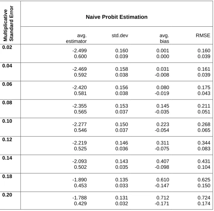
Let us first consider the results of the naive probit estimation (Table 1). The stan-dard errors of the multiplicative noise are given in the first column. In addition to the average estimator and the standard deviation we display also the average bias and root mean squared error (RMSE). The higher the value of the standard error of the multiplicative measurement error, the greater the bias of the naive esti-mates becomes, as expected. The RMSE rises strongly with the perturbation degree.

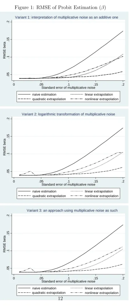
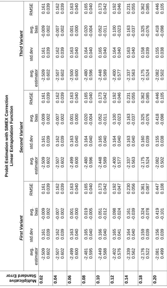
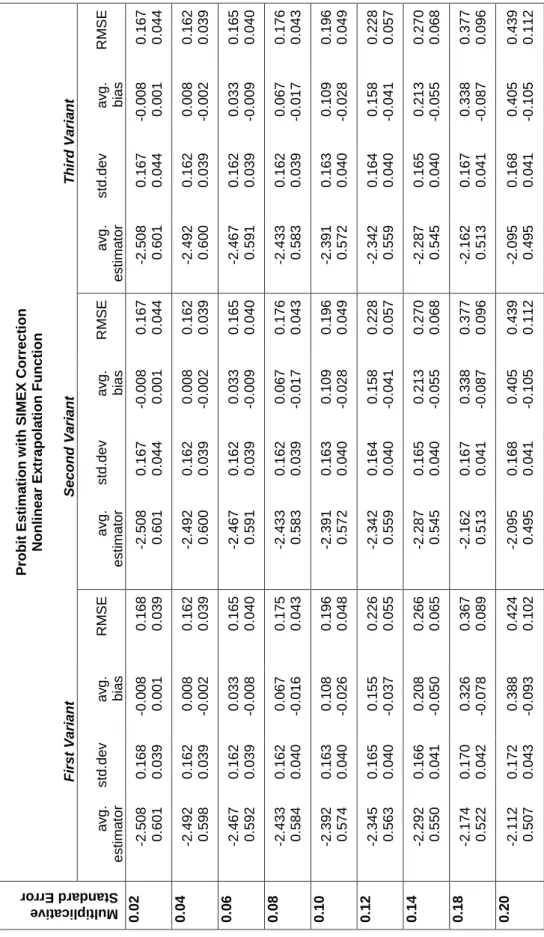
The simulation results of the SIMEX estimation are given in Tables 2, 3 and 4. We see that in all experiments, the SIMEX procedure is able to reduce the bias due to the presence of multiplicative measurement error. Figure 1 shows the RMSE of the point estimate β depending on the standard error of the multiplicative noise σ_w2.6 Compared with the results of the naive estimation, the RMSE obtained with the SIMEX estimation procedure is considerably reduced regardless which extrapolation function or which variant was used.

In the following we analyze only the results of the SIMEX estimation. Comparing the results in Figure 1 and Tables 2, 3 and 4, we can detect only slight differences between three variants. However, the choice of a certain extrapolation function has a strong impact on the results.

Now, let us consider which extrapolation function yields the best results. With small errors (σw = 0.02), there are no significant differences.7 The quadratic extrapolation

function is superior to the other functions. Beforeσw reaches 0.12 (at this point the

measurement error is already fairly high), the corrected estimators are very close to the true value. The linear function is second best. It delivers good correction results if the error is middling (σw about 0.06). The nonlinear function fares worst.

However, when the error is very large (σw = 0.2) the nonlinear function comes closer

to the linear one.

Thus, the quality of the estimation depends on the choice of the extrapolation func-tion. In addition to that, the margin of error also plays a role. With minimal noise (σw = 0.02) the differences between the variants and extrapolation functions are also

6_{The development forαis similar and therefore not reported here.}

7_{However, the nonlinear extrapolation function in variants 2 and 3 has an outlier at the point}

minimal (except for an outlier in variants 2 and 3 with the nonlinear extrapolation function). If we increase the range to middling (σw = 0.06), only quadratic and

lin-ear extrapolation functions work well. If the multiplicative noise is high (σw = 0.08

Table 1: Naive Probit Estimation

Naive Probit Estimation

M u lt ip li c a ti v e S ta n d a rd E rr o r avg. estimator std.dev avg. bias RMSE 0.02 -2.499 0.600 0.160 0.039 0.001 0.000 0.160 0.039 0.04 -2.469 0.592 0.158 0.038 0.031 -0.008 0.161 0.039 0.06 -2.420 0.581 0.156 0.038 0.080 -0.019 0.175 0.043 0.08 -2.355 0.565 0.153 0.037 0.145 -0.035 0.211 0.051 0.10 -2.277 0.546 0.150 0.037 0.223 -0.054 0.268 0.065 0.12 -2.219 0.525 0.146 0.036 0.311 -0.075 0.344 0.083 0.14 -2.093 0.502 0.143 0.035 0.407 -0.098 0.431 0.104 0.18 -1.890 0.453 0.135 0.033 0.610 -0.147 0.625 0.150 0.20 -1.788 0.429 0.131 0.032 0.712 -0.171 0.724 0.174

Figure 1: RMSE of Probit Estimation (β) .0 5 .1 .1 5 .2 R M S E b e ta 0 .05 .1 .15 .2

Standard error of multiplicative noise

naive estimation linear extrapolation quadratic extrapolation nonlinear extrapolation Variant 1: interpretation of multiplicative noise as an additive one

.0 5 .1 .1 5 .2 R M S E b e ta 0 .05 .1 .15 .2

Standard error of multiplicative noise

naive estimation linear extrapolation quadratic extrapolation nonlinear extrapolation Variant 2: logarithmic transformation of multiplicative noise

.0 5 .1 .1 5 .2 R M S E b e ta 0 .05 .1 .15 .2

Standard error of multiplicative noise

naive estimation linear extrapolation quadratic extrapolation nonlinear extrapolation Variant 3: an approach using multiplicative noise as such

Table 2: Simulation Results: SIMEX with Linear Extrapolation P ro b it E s ti m a ti o n w it h S IM E X C o rr e c ti o n L in e a r E x tr a p o la ti o n F u n c ti o n F ir s t V a ri a n t S e c o n d V a ri a n t T h ir d V a ri a n t Mu lti pli ca tiv e Sta nd ard E rro r a v g . e s ti m a to r s td .d e v a v g . b ia s R M S E a v g . e s ti m a to r s td .d e v a v g . b ia s R M S E a v g . e s ti m a to r s td .d e v a v g . b ia s R M S E 0 .0 2 -2 .5 0 9 0 .6 0 2 0 .1 6 1 0 .0 3 9 -0 .0 0 9 0 .0 0 2 0 .1 6 1 0 .0 3 9 -2 .5 0 9 0 .6 0 2 0 .1 6 1 0 .0 3 9 -0 .0 0 9 0 .0 0 2 0 .1 6 1 0 .0 3 9 -2 .5 0 9 0 .6 0 2 0 .1 6 1 0 .0 3 9 -0 .0 0 9 0 .0 0 2 0 .1 6 1 0 .0 3 9 0 .0 4 -2 .5 0 7 0 .6 0 2 0 .1 6 2 0 .0 3 9 -0 .0 0 7 0 .0 0 2 0 .1 6 2 0 .0 3 9 -2 .5 0 7 0 .6 0 2 0 .1 6 2 0 .0 3 9 -0 .0 0 7 0 .0 0 2 0 .1 6 2 0 .0 3 9 -2 .5 0 7 0 .6 0 2 0 .1 6 2 0 .0 3 9 -0 .0 0 7 0 .0 0 2 0 .1 6 2 0 .0 3 9 0 .0 6 -2 .4 9 9 0 .6 0 0 0 .1 6 3 0 .0 4 0 0 .0 0 1 -0 .0 0 0 0 .1 6 3 0 .0 4 0 -2 .4 9 9 0 .6 0 0 0 .1 6 3 0 .0 4 0 0 .0 0 1 0 .0 0 0 0 .1 6 3 0 .0 4 0 -2 .5 0 0 0 .6 0 0 0 .1 6 3 0 .0 4 0 0 .0 0 1 0 .0 0 0 0 .1 6 3 0 .0 4 0 0 .0 8 -2 .4 8 1 0 .5 9 5 0 .1 6 5 0 .0 4 0 0 .0 1 9 -0 .0 0 5 0 .1 6 5 0 .0 4 0 -2 .4 8 0 0 .5 9 6 0 .1 6 4 0 .0 4 0 0 .0 2 0 -0 .0 0 4 0 .1 6 5 0 .0 4 0 -2 .4 8 0 0 .5 9 6 0 .1 6 4 0 .0 4 0 0 .0 2 0 -0 .0 0 4 0 .1 6 5 0 .0 4 0 0 .1 0 -2 .4 4 9 0 .5 8 8 0 .1 6 6 0 .0 4 0 0 .0 5 1 -0 .0 1 2 0 .1 7 3 0 .0 4 2 -2 .4 4 8 0 .5 8 9 0 .1 6 5 0 .0 4 0 0 .0 5 2 -0 .0 1 1 0 .1 7 3 0 .0 4 2 -2 .4 4 8 0 .5 8 9 0 .1 6 5 0 .0 4 0 0 .0 5 2 -0 .0 1 1 0 .1 7 3 0 .0 4 2 0 .1 2 -2 .4 0 2 0 .5 7 6 0 .1 6 5 0 .0 4 1 0 .0 9 8 -0 .0 2 4 0 .1 9 2 0 .0 4 7 -2 .4 0 0 0 .5 7 7 0 .1 6 4 0 .0 4 0 0 .1 0 0 -0 .0 2 3 0 .1 9 2 0 .0 4 6 -2 .4 0 0 0 .5 7 7 0 .1 6 4 0 .0 4 0 0 .1 0 0 -0 .0 2 3 0 .1 9 2 0 .0 4 6 0 .1 4 -2 .3 3 9 0 .5 6 2 0 .1 6 4 0 .0 4 0 0 .1 6 1 -0 .0 3 9 0 .2 3 0 0 .0 5 6 -2 .3 3 7 0 .5 6 3 0 .1 6 3 0 .0 4 0 0 .1 6 3 -0 .0 3 7 0 .2 3 1 0 .0 5 5 -2 .3 3 7 0 .5 6 3 0 .1 6 3 0 .0 4 0 0 .1 6 3 -0 .0 3 7 0 .2 3 1 0 .0 5 5 0 .1 8 -2 .1 7 6 0 .5 2 2 0 .1 5 9 0 .0 3 9 0 .3 2 4 -0 .0 7 8 0 .3 6 1 0 .0 8 7 -2 .1 7 5 0 .5 2 4 0 .1 6 0 0 .0 3 9 0 .3 2 5 -0 .0 7 6 0 .3 6 2 0 .0 8 5 -2 .1 7 5 0 .5 2 4 0 .1 5 8 0 .0 3 9 0 .3 2 5 -0 .0 7 6 0 .3 6 2 0 .0 8 5 0 .2 0 -2 .0 8 1 0 .4 9 9 0 .1 5 6 0 .0 3 9 0 .4 1 9 -0 .1 0 1 0 .4 4 7 0 .1 0 8 -2 .0 8 2 0 .5 0 2 0 .1 5 5 0 .0 3 8 0 .4 1 8 -0 .0 9 8 0 .4 4 6 0 .1 0 5 -2 .0 8 2 0 .5 0 2 0 .1 5 5 0 .0 3 8 0 .4 1 8 -0 .0 9 8 0 .4 4 6 0 .1 0 5

Table 3: Simulation Results: SIMEX with Quadratic Extrapolation P ro b it E s ti m a ti o n w it h S IM E X C o rr e c ti o n Q u a d ra ti c E x tr a p o la ti o n F u n c ti o n F ir s t V a ri a n t S e c o n d V a ri a n t T h ir d V a ri a n t Mu lti pli ca tiv e Sta nd ard E rro r a v g . e s ti m a to r s td .d e v a v g . b ia s R M S E a v g . e s ti m a to r s td .d e v a v g . b ia s R M S E a v g . e s ti m a to r s td .d e v a v g . b ia s R M S E 0 .0 2 -2 .5 0 9 0 .6 0 2 0 .1 6 1 0 .0 3 9 -0 .0 0 9 0 .0 0 2 0 .1 6 1 0 .0 3 9 -2 .5 0 9 0 .6 0 2 0 .1 6 1 0 .0 3 9 -0 .0 0 9 0 .0 0 2 0 .1 6 1 0 .0 3 9 -2 .5 0 9 0 .6 0 2 0 .1 6 1 0 .0 3 9 -0 .0 0 9 0 .0 0 2 0 .1 6 1 0 .0 3 9 0 .0 4 -2 .5 0 9 0 .6 0 2 0 .1 6 2 0 .0 3 9 -0 .0 0 9 0 .0 0 2 0 .1 6 2 0 .0 3 9 -2 .5 0 9 0 .6 0 2 0 .1 6 2 0 .0 3 9 -0 .0 0 9 0 .0 0 2 0 .1 6 2 0 .0 3 9 -2 .5 0 9 0 .6 0 2 0 .1 6 2 0 .0 3 9 -0 .0 0 9 0 .0 0 2 0 .1 6 2 0 .0 3 9 0 .0 6 -2 .5 0 9 0 .6 0 2 0 .1 6 4 0 .0 4 0 -0 .0 0 9 0 .0 0 2 0 .1 6 4 0 .0 4 0 -2 .5 0 8 0 .6 0 1 0 .1 6 4 0 .0 4 0 -0 .0 0 8 0 .0 0 1 0 .1 6 4 0 .0 4 0 -2 .5 0 8 0 .6 0 1 0 .1 6 4 0 .0 4 0 -0 .0 0 8 0 .0 0 1 0 .1 6 4 0 .0 4 0 0 .0 8 -2 .5 0 7 0 .6 0 2 0 .1 6 8 0 .0 4 1 -0 .0 0 7 0 .0 0 2 0 .1 6 8 0 .0 4 1 -2 .5 0 6 0 .6 0 1 0 .1 6 8 0 .0 4 1 -0 .0 0 6 0 .0 0 1 0 .1 6 8 0 .0 4 1 -2 .5 0 6 0 .6 0 1 0 .1 6 8 0 .0 4 1 -0 .0 0 6 0 .0 0 1 0 .1 6 8 0 .0 4 1 0 .1 0 -2 .5 0 3 0 .6 0 1 0 .1 7 2 0 .0 4 2 -0 .0 0 3 0 .0 0 1 0 .1 7 2 0 .0 4 2 -2 .5 0 0 0 .5 9 9 0 .1 7 2 0 .0 4 2 0 .0 0 0 -0 .0 0 1 0 .1 7 1 0 .0 4 2 -2 .5 0 0 0 .5 9 9 0 .1 7 2 0 .0 4 2 0 .0 0 0 0 .0 0 0 0 .1 7 1 0 .0 4 2 0 .1 2 -2 .4 9 2 0 .5 9 8 0 .1 7 7 0 .0 4 4 0 .0 0 8 -0 .0 0 2 0 .1 7 7 0 .0 4 4 -2 .4 8 7 0 .5 9 5 0 .1 7 6 0 .0 4 3 0 .0 1 3 -0 .0 0 5 0 .1 7 6 0 .0 4 3 -2 .4 8 7 0 .5 9 5 0 .1 7 6 0 .0 4 3 0 .0 1 3 -0 .0 0 5 0 .1 7 6 0 .0 4 3 0 .1 4 -2 .4 7 3 0 .5 9 4 0 .1 8 1 0 .0 4 5 0 .0 2 7 -0 .0 0 6 0 .1 8 3 0 .0 4 5 -2 .4 6 6 0 .6 0 0 0 .1 8 0 0 .0 4 4 0 .0 3 4 -0 .0 1 0 0 .1 8 2 0 .0 4 5 -2 .4 6 6 0 .5 9 0 0 .1 7 9 0 .0 4 4 0 .0 3 4 -0 .0 1 0 0 .1 8 2 0 .0 4 5 0 .1 8 -2 .4 0 5 0 .5 7 7 0 .1 8 8 0 .0 4 7 0 .0 9 5 -0 .0 2 3 0 .2 1 0 0 .0 5 2 -2 .3 9 1 0 .5 7 1 0 .1 8 4 0 .0 4 6 0 .1 0 9 -0 .0 2 9 0 .2 1 4 0 .0 5 4 -2 .3 9 1 0 .5 7 1 0 .1 8 4 0 .0 4 6 0 .1 0 9 -0 .0 2 9 0 .2 1 4 0 .0 5 4 0 .2 0 -2 .3 5 5 0 .5 6 5 0 .1 9 0 0 .0 4 8 0 .1 4 5 -0 .0 3 5 0 .2 3 9 0 .0 5 9 -2 .3 3 8 0 .5 5 8 0 .1 8 6 0 .0 4 6 0 .1 6 2 -0 .0 4 2 0 .2 4 7 0 .0 6 2 -2 .3 3 8 0 .5 5 8 0 .1 8 6 0 .0 4 6 0 .1 6 2 -0 .0 4 2 0 .2 4 7 0 .0 6 2

Table 4: Simulation Results: SIMEX with Nonlinear Extrapolation P ro b it E s ti m a ti o n w it h S IM E X C o rr e c ti o n N o n li n e a r E x tr a p o la ti o n F u n c ti o n F ir s t V a ri a n t S e c o n d V a ri a n t T h ir d V a ri a n t Mu lti pli ca tiv e Sta nd ard E rro r a v g . e s ti m a to r s td .d e v a v g . b ia s R M S E a v g . e s ti m a to r s td .d e v a v g . b ia s R M S E a v g . e s ti m a to r s td .d e v a v g . b ia s R M S E 0 .0 2 -2 .5 0 8 0 .6 0 1 0 .1 6 8 0 .0 3 9 -0 .0 0 8 0 .0 0 1 0 .1 6 8 0 .0 3 9 -2 .5 0 8 0 .6 0 1 0 .1 6 7 0 .0 4 4 -0 .0 0 8 0 .0 0 1 0 .1 6 7 0 .0 4 4 -2 .5 0 8 0 .6 0 1 0 .1 6 7 0 .0 4 4 -0 .0 0 8 0 .0 0 1 0 .1 6 7 0 .0 4 4 0 .0 4 -2 .4 9 2 0 .5 9 8 0 .1 6 2 0 .0 3 9 0 .0 0 8 -0 .0 0 2 0 .1 6 2 0 .0 3 9 -2 .4 9 2 0 .6 0 0 0 .1 6 2 0 .0 3 9 0 .0 0 8 -0 .0 0 2 0 .1 6 2 0 .0 3 9 -2 .4 9 2 0 .6 0 0 0 .1 6 2 0 .0 3 9 0 .0 0 8 -0 .0 0 2 0 .1 6 2 0 .0 3 9 0 .0 6 -2 .4 6 7 0 .5 9 2 0 .1 6 2 0 .0 3 9 0 .0 3 3 -0 .0 0 8 0 .1 6 5 0 .0 4 0 -2 .4 6 7 0 .5 9 1 0 .1 6 2 0 .0 3 9 0 .0 3 3 -0 .0 0 9 0 .1 6 5 0 .0 4 0 -2 .4 6 7 0 .5 9 1 0 .1 6 2 0 .0 3 9 0 .0 3 3 -0 .0 0 9 0 .1 6 5 0 .0 4 0 0 .0 8 -2 .4 3 3 0 .5 8 4 0 .1 6 2 0 .0 4 0 0 .0 6 7 -0 .0 1 6 0 .1 7 5 0 .0 4 3 -2 .4 3 3 0 .5 8 3 0 .1 6 2 0 .0 3 9 0 .0 6 7 -0 .0 1 7 0 .1 7 6 0 .0 4 3 -2 .4 3 3 0 .5 8 3 0 .1 6 2 0 .0 3 9 0 .0 6 7 -0 .0 1 7 0 .1 7 6 0 .0 4 3 0 .1 0 -2 .3 9 2 0 .5 7 4 0 .1 6 3 0 .0 4 0 0 .1 0 8 -0 .0 2 6 0 .1 9 6 0 .0 4 8 -2 .3 9 1 0 .5 7 2 0 .1 6 3 0 .0 4 0 0 .1 0 9 -0 .0 2 8 0 .1 9 6 0 .0 4 9 -2 .3 9 1 0 .5 7 2 0 .1 6 3 0 .0 4 0 0 .1 0 9 -0 .0 2 8 0 .1 9 6 0 .0 4 9 0 .1 2 -2 .3 4 5 0 .5 6 3 0 .1 6 5 0 .0 4 0 0 .1 5 5 -0 .0 3 7 0 .2 2 6 0 .0 5 5 -2 .3 4 2 0 .5 5 9 0 .1 6 4 0 .0 4 0 0 .1 5 8 -0 .0 4 1 0 .2 2 8 0 .0 5 7 -2 .3 4 2 0 .5 5 9 0 .1 6 4 0 .0 4 0 0 .1 5 8 -0 .0 4 1 0 .2 2 8 0 .0 5 7 0 .1 4 -2 .2 9 2 0 .5 5 0 0 .1 6 6 0 .0 4 1 0 .2 0 8 -0 .0 5 0 0 .2 6 6 0 .0 6 5 -2 .2 8 7 0 .5 4 5 0 .1 6 5 0 .0 4 0 0 .2 1 3 -0 .0 5 5 0 .2 7 0 0 .0 6 8 -2 .2 8 7 0 .5 4 5 0 .1 6 5 0 .0 4 0 0 .2 1 3 -0 .0 5 5 0 .2 7 0 0 .0 6 8 0 .1 8 -2 .1 7 4 0 .5 2 2 0 .1 7 0 0 .0 4 2 0 .3 2 6 -0 .0 7 8 0 .3 6 7 0 .0 8 9 -2 .1 6 2 0 .5 1 3 0 .1 6 7 0 .0 4 1 0 .3 3 8 -0 .0 8 7 0 .3 7 7 0 .0 9 6 -2 .1 6 2 0 .5 1 3 0 .1 6 7 0 .0 4 1 0 .3 3 8 -0 .0 8 7 0 .3 7 7 0 .0 9 6 0 .2 0 -2 .1 1 2 0 .5 0 7 0 .1 7 2 0 .0 4 3 0 .3 8 8 -0 .0 9 3 0 .4 2 4 0 .1 0 2 -2 .0 9 5 0 .4 9 5 0 .1 6 8 0 .0 4 1 0 .4 0 5 -0 .1 0 5 0 .4 3 9 0 .1 1 2 -2 .0 9 5 0 .4 9 5 0 .1 6 8 0 .0 4 1 0 .4 0 5 -0 .1 0 5 0 .4 3 9 0 .1 1 2

5

Conclusion

In this paper we compare three variants to specify the multiplicative measurement error model in the simulation step of the SIMEX method. The choice of the SIMEX approach allows us to consider linear or nonlinear regression models with multiplica-tive measurement error, because this approach does not depend on the functional form of the model. The only restriction we have in our approach is that the vari-ance of the multiplicative measurement error has to be known. The Monte Carlo experiments show that all three variants work equally well and that the quality of the estimation depends only on the choice of the extrapolation function as well as on the margin of the measurement error. In the light of our Monte Carlo results, we see also that it is always better to use several extrapolation functions and not to restrict oneself to a specific one from the beginning on, as for example the quadratic one which is principally used in applied works, since each of them seems to perform better for a certain values of the variance of the measurement error.

Since our approach is purely descriptive and leaves a lot of questions open a final conclusion concerning the relative ability of the different variants to estimate the parameters of the true data generating process, if multiplicative measurement error occurs, is somewhat premature. More Monte Carlo evidence on various nonlinear and linear regression models is needed. First, in this paper we considered the case of positive noise. From a methodic point of view it might be of interest to analyze how the variants 1 and 3 perform in the the case of uniformly or normally distributed measurement error which adopts also negative values. Second, other specifications of the extrapolation function (for instance, an exponential one) might be used in order to mimic better the relationship between the naive estimates and the control parameter for the variance of the measurement error. Finally, in order to take the outliers or in other words the extreme values of the covariates generated during the simulation step of the algorithm better into account, it will be useful to consider the median of the estimates instead of their mean; this is in progress.

References

Carroll, R., H. Kuechenhoff, F. Lombard, and L. Stefanski (1996):

“Asymptotics for the Simex Estimator in Structural Measurement Error Mod-els,” Journal of the American Statistical Association, 91, 242–250.

Carroll, R., D. Ruppert, and L. Stefanski (1995): Measurement Error in

Nonlinear Models. Chapman and Hall.

Cook, J., and L. Stefanski (1994): “A Simulation Extrapolation Method for

Parametric Measurement Error Models,”Journal of the American Statistical As-sociation, 89, 1314–1328.

Fuller, W.(1987): Measurement Error Models. Wiley.

Hwang, J. T.(1986): “Multiplicative Errors-in-Variables Models with Applications

to Recent Data Released by the U.S. Department of Energy,” Journal of the American Statistical Association, 81, 680–688.

Iturria, S., R. Carroll,and D. Firth(1999): “Polynomial Regression and

Es-timating Functions in the Presence of Multiplicative Measurement Error,”Journal of the Royal Statistical Society. Series B (Statistical Methodology), 61, 547 – 561.

Lin, A.(1989): “Estimation of Multiplicative Measurement-Error Models and Some

Simulation Results,” Economics Letters, 317, 13–20.

Lyles, R., and L. Kupper(1997): “A Detailed Evaluation of Adjustment

Meth-ods for Multiplicative Measurement Error in Linear Regression with Applications in Occupational Epidemiology,” Biometrics, 53, 1008–1025.

Nolte, S.(2007): “The Multiplicative Simulation Extrapolation Approach,”

Work-ing Paper, University of Konstanz.

Ronning, G., R. Sturm, J. Hoehne, R. Lenz, M. Rosemann, M.

Schef-fler, and D. Vorgrimler (2005): Handbuch zur Anonymisierung

wirtschaf-sstatistischer Mikrodaten. Statistiches Bundesamt: Statistik und Wissenschaft, Band 4.

Rosemann, M. (2006): Auswirkungen datenverndernder

Anonymisierungsver-fahren auf die Analyse von Mikrodaten. Institut fuer Angewandte Wirtschafts-fotschung: IAW-Report, Nr. 66.

Schafer, D. (1990): “Measurement Error Model Estimation using iteratively

weighted least squares,” in Brown P.J. and Fuller W.A. : Contemporary Mathe-matics, Providence Rhode Island, American Mathematical Society.

Stefanski, L., and J. Cook (1995): “Simulation-Extrapolation: The

Measure-ment Error Jackknife,” Journal of the American Statistical Association, 90(432), 1247–1256.

IAW-Diskussionspapiere

Bisher erschienen:

Nr. 1 (September 2001)

Das Einstiegsgeld – eine zielgruppenorientierte negative Einkommensteuer: Konzeption, Umsetzung und eine erste Zwischenbilanz nach 15 Monaten in Baden-Württemberg

Sabine Dann / Andrea Kirchmann / Alexander Spermann / Jürgen Volkert

Nr. 2 (Dezember 2001)

Die Einkommensteuerreform 1990 als natürliches Experiment. Methodische und konzeptionelle Aspekte zur Schätzung der Elastizität des zu versteuernden Einkommens

Peter Gottfried / Hannes Schellhorn

Nr. 3 (Januar 2001)

Gut betreut in den Arbeitsmarkt? Eine mikroökonomische Evaluation der Mannheimer Arbeitsvermittlungsagentur

Jürgen Jerger / Christian Pohnke / Alexander Spermann

Nr. 4 (Dezember 2001)

Das IAW-Einkommenspanel und das Mikrosimulationsmodell SIMST

Peter Gottfried / Hannes Schellhorn

Nr. 5 (April 2002)

A Microeconometric Characterisation of Household Consumption Using Quantile Regression

Niels Schulze / Gerd Ronning

Nr. 6 (April 2002)

Determinanten des Überlebens von Neugründungen in der baden-württembergischen Industrie – eine empirische Survivalanalyse mit amtlichen Betriebsdaten

Harald Strotmann

Nr. 7 (November 2002)

Die Baulandausweisungsumlage als ökonomisches Steuerungsinstrument einer nachhaltigkeitsorientierten Flächenpolitik

Raimund Krumm

Nr. 8 (März 2003)

Making Work Pay: U.S. American Models for a German Context?

Laura Chadwick, Jürgen Volkert

Nr. 9 (Juni 2003)

Erste Ergebnisse von vergleichenden Untersuchungen mit anonymisierten und nicht anonymisierten Einzeldaten am Beispiel der Kostenstrukturerhebung und der Umsatzsteuerstatistik

Martin Rosemann

Nr. 10 (August 2003)

Randomized Response and the Binary Probit Model

IAW-Diskussionspapiere

Nr. 11 (August 2003)

Creating Firms for a New Century: Determinants of Firm Creation around 1900

Joerg Baten

Nr. 12 (September 2003)

Das fiskalische BLAU-Konzept zur Begrenzung des Siedlungsflächenwachstums

Raimund Krumm

Nr. 13 (Dezember 2003)

Generelle Nichtdiskontierung als Bedingung für eine nachhaltige Entwicklung?

Stefan Bayer

Nr. 14 (Februar 2003)

Die Elastizität des zu versteuernden Einkommens. Messung und erste Ergebnisse zur empirischen Evidenz für die Bundesrepublik Deutschland.

Peter Gottfried / Hannes Schellhorn

Nr. 15 (Februar 2004)

Empirical Evidence on the Effects of Marginal Tax Rates on Income – The German Case

Peter Gottfried / Hannes Schellhorn

Nr. 16 (Juli 2004)

Shadow Economies around the World: What do we really know?

Friedrich Schneider

Nr. 17 (August 2004)

Firm Foundations in the Knowledge Intensive Business Service Sector. Results from a Comparative Empirical Study in Three German Regions

Andreas Koch / Thomas Stahlecker

Nr. 18 (Januar 2005)

The impact of functional integration and spatial proximity on the post-entry performance of knowledge intensive business service firms

Andreas Koch / Harald Strotmann

Nr. 19 (März 2005)

Legislative Malapportionment and the Politicization of Germany’s Intergovernmental Transfer System

Hans Pitlik / Friedrich Schneider / Harald Strotmann

Nr. 20 (April 2005)

Implementation ökonomischer Steuerungsansätze in die Raumplanung

Raimund Krumm

Nr. 21 (Juli 2005)

Determinants of Innovative Activity in Newly Founded Knowledge Intensive Business Service Firms

Andreas Koch / Harald Strotmann

Nr. 22 (Dezember 2005)

Impact of Opening Clauses on Bargained Wages

IAW-Diskussionspapiere

Nr. 23 (Januar 2006)

Hat die Einführung von Gewinnbeteiligungsmodellen kurzfristige positive

Produktivitätswirkungen? – Ergebnisse eines Propensity-Score-Matching-Ansatzes

Harald Strotmann

Nr. 24 (März 2006)

Who Goes East? The Impact of Enlargement on the Pattern of German FDI

Claudia M. Buch / Jörn Kleinert

Nr. 25 (Mai 2006)

Estimation of the Probit Model from Anonymized Micro Data

Gerd Ronning / Martin Rosemann

Nr. 26 (Oktober 2006)

Bargained Wages in Decentralized Wage-Setting Regimes

Wolf Dieter Heinbach

Nr. 27 (Januar 2007)

A Capability Approach for Official German Poverty and Wealth Reports: Conceptual Background and First Empirical Results

Christian Arndt / Jürgen Volkert

Nr. 28 (Februar 2007)

Typisierung der Tarifvertragslandschaft – Eine Clusteranalyse der tarif- vertraglichen Öffnungsklauseln

Wolf Dieter Heinbach / Stefanie Schröpfer

Nr. 29 (März 2007)

International Bank Portfolios: Short- and Long-Run Responses to the Business Cycles

Sven Blank / Claudia M. Buch

Nr. 30 (April 2007)

Stochastische Überlagerungen mit Hilfe der Mischungsverteilung

Gerd Ronning

Nr. 31 (Mai 2007)

Openness and Growth: The Long Shadow of the Berlin Wall

Claudia M. Buch / Farid Toubal

Nr. 32 (Mai 2007)

International Banking and the Allocation of Risk

Claudia M. Buch / Gayle DeLong / Katja Neugebauer

Nr. 33 (Juli 2007)

Multinational Firms and New Protectionisms

IAW-Diskussionspapiere

Nr. 34 (November 2007)

Within-Schätzung bei anonymisierten Paneldaten

Elena Biewen

Nr. 35 (Dezember 2007)

What a Difference Trade Makes – Export Activity and the Flexibility of Collective Bargaining Agreements

Wolf Dieter Heinbach / Stefanie Schröpfer

Nr. 36 (Dezember 2007)

To Bind or Not to Bind Collectively? Decomposition of Bargained Wage Differences Using Counterfactual Distributions

Wolf Dieter Heinbach / Markus Spindler

Nr. 37 (Dezember 2007)

Neue Ansätze zur flächenschutzpolitischen Reform des

Kommunalen Finanzausgleichs

Raimund Krumm

Nr. 38 (Januar 2008)

Banking Globalization: International Consolidation and Mergers in Banking

Claudia M. Buch / Gayle L. DeLong

Nr. 39 (Januar 2008)

Multiplicative Measurement Error and the Simulation Extrapolation Method