UR Scholarship Repository
Physics Faculty Publications
Physics
1-27-2017
Analysis of a Custom Support Vector Machine for
Photometric Redshift Estimation and the Inclusion
of Galaxy Shape Information
Jack Singal
University of Richmond, [email protected]
Evan Jones
University of Richmond
Follow this and additional works at:
https://scholarship.richmond.edu/physics-faculty-publications
Part of the
Physics Commons
This Article is brought to you for free and open access by the Physics at UR Scholarship Repository. It has been accepted for inclusion in Physics Faculty Publications by an authorized administrator of UR Scholarship Repository. For more information, please contact
Recommended Citation
Evan Jones and Jack Singa. "Analysis of a Custom Support Vector Machine for Photometric Redshift Estimation and the Inclusion of Galaxy Shape Information."Astronomy & Astrophysics600, A113 (2017), 1-1. doi: 10.1051/0004-6361/201629558.
A&A 600, A113 (2017) DOI:10.1051/0004-6361/201629558 c ESO 2017
Astronomy
&
Astrophysics
Analysis of a custom support vector machine for photometric
redshift estimation and the inclusion of galaxy shape information
E. Jones and J. Singal
Physics Department, University of Richmond 28 Westhampton Way, University of Richmond, VA 23173, USA e-mail:[email protected]
Received 20 August 2016/Accepted 27 January 2017
ABSTRACT
Aims.We present a custom support vector machine classification package for photometric redshift estimation, including compar-isons with other methods. We also explore the efficacy of including galaxy shape information in redshift estimation. Support vector machines, a type of machine learning, utilize optimization theory and supervised learning algorithms to construct predictive models based on the information content of data in a way that can treat different input features symmetrically, which can be a useful estimator of the information contained in additional features beyond photometry, such as those describing the morphology of galaxies.
Methods.The custom support vector machine package we have developed is designated SPIDERz and made available to the com-munity. As test data for evaluating performance and comparison with other methods, we apply SPIDERz to four distinct data sets: 1) the publicly available portion of the PHAT-1 catalog based on the GOODS-N field with spectroscopic redshifts in the rangez<3.6, 2) 14 365 galaxies from the COSMOS bright survey with photometric band magnitudes, morphology, and spectroscopic redshifts insidez<1.4, 3) 3048 galaxies from the overlap of COSMOS photometry and morphology with 3D-HST spectroscopy extending to
z<3.9, and 4) 2612 galaxies with five-band photometric magnitudes and morphology from the All-wavelength Extended Groth Strip International Survey andz<1.57.
Results.We find that SPIDERz achieves results competitive with other empirical packages on the PHAT-1 data, and performs quite well in estimating redshifts with the COSMOS and AEGIS data, including in the cases of a large redshift range (0<z <3.9). We also determine from analyses with both the COSMOS and AEGIS data that the inclusion of morphological information does not have a statistically significant benefit for photometric redshift estimation with the techniques employed here.
Key words. techniques: photometric – galaxies: statistics – methods: miscellaneous
1. Introduction
An important challenge for the current and coming era of large multi-band extragalactic surveys is obtaining sufficiently accu-rate photometric redshift estimates and understanding the error properties of these estimates (see e.g.Huterer et al. 2006, for a review). Unlike time consuming spectroscopic redshift determi-nation, photometric redshift estimation (photo-z) is subject to significant systematic errors and confusion because the spectral information of a galaxy is limited to the magnitude or flux in a number of wavelength bands. When photo-zs are used, science goals such as using weak lensing for cosmology are strongly affected by the number of outliers – those objects whose esti-mated photo-zs are far from the actual redshifts (e.g.Hearin et al. 2010). In general, data sets with bands extending into those ob-served by infrared telescopes (e.g. J, H, and K bands) have more accurate photo-zestimation and fewer outliers. However, most upcoming large surveys, such as the Large Synoptic Sur-vey Telescope (LSST,Ivezic et al. 2008), will have optical and near-infrared data only. Reducing the number of, and potentially having a method of identifying, the potential outliers in photo-z
estimation is an important goal for these projects.
Photo-z estimation techniques have traditionally been di-vided into two main classifications. So-called “Template fit-ting” methods, such as the Lephare package as described in Ilbert et al. (2006) and Arnouts et al. (1999), and Bayesian Photometric Redshift (BPZ) as described in Benítez (2000),
involve correlating the observed band photometry with model galaxy spectra and redshift, and possibly other model prop-erties. So-called “Empirical” or “Training set” methods, such as artificial neural networks (e.g. ANNz, Collister & Lahav
2004), boosted decision trees (e.g. ArborZ, Gerdes et al.
2010), regression trees/random forests (e.g.Carliles et al. 2010;
Carrasco Kind & Bruner 2013), support vector machines (e.g.
Wadadekar 2004), polynomial mapping (e.g. Budavari et al. 2005;Li & Yee 2008), and others develop a mapping from input parameters to redshift with a training set of data in which the ac-tual spectroscopic redshifts are known, then apply the mappings to data for which the redshifts are to be estimated. Both have their drawbacks – template fitting methods require assumptions about intrinsic galaxy spectra or their redshift evolution, and em-pirical methods require the training set to be “complete” in the sense that it is representative of the target evaluation population in bulk in all characteristics. In a previous work (Singal et al. 2011) we reported on a custom artificial neural network algo-rithm for photometric redshift determination.
Because of the larger frequency of mergers at higher red-shifts and the general evolutionary trend from spiral to elliptical shapes among galaxies, it is a reasonable hypothesis that galaxy morphology and redshift are correlated in such a way that the ad-dition of morphological information could improve photo-z es-timation. The inclusion of morphological parameters in
photo-zestimation has been studied using Sloan Digital Sky Survey (SDSS) data byTagliaferri et al.(2003) with an artificial neural
network determination, and by Vince & Csabai (2007) and
Way & Srivastava (2006) with other methods.Tagliaferri et al.
(2003) find possible modest improvement with the inclusion of shape information, although they restrict their analysis to quite low redshift (z ≤0.7) galaxies.Way & Srivastava(2006) con-sider several empirical methods and show marginal improve-ment for some methods with the addition of morphological information. Vince & Csabai (2007) claim an improvement of between 1 and 3 percent in the RMS error in photo-z determina-tion, however it is not noted whether this result is significant and the method of photo-zestimation is not discussed.Singal et al.
(2011) considered one of the galaxy test data sets used here which includes a more thorough sample of higher redshift galax-ies extending toz∼1.57 and found that including galaxy shape information did not result in a statistically significant benefit in the context of a neural network method.
In this work, we evaluate the performance of a custom sup-port vector machine (SVM) package for photo-zdetermination with comparisons to other photo-zalgorithms, and also explore the efficacy of integrating parameters describing the morpho-logical information of galaxies. The SVM package used in this analysis is developed for the IDL environment by one of the au-thors (EJ), based largely on algorithmic procedures outlined in
Chang & Lin (2011), and has been named SPIDERz (SuPport vector classification for IDEntifying Redshifts)1. It can include additional parameters beyond photometry, such as morphologi-cal information, on an equal footing.
Here we follow convention (e.g.Hildebrandt et al. 2010) and define “outliers” as those galaxies where
Outliers: |zphot−zspec| 1+zspec
> .15, (1)
wherezphotandzspecare the estimated photo-zand actual
(spec-troscopically determined) redshift of the object. The RMS
photo-zerror in a realization is given by a standard definition
σ∆z/(1+z) ≡ s 1 ngalsΣ gals zphot−zspec 1+zspec !2 , (2)
wherengals is the number of galaxies in the evaluation set and
Σgalsrepresents a sum over those galaxies. For comparison with
other works, we also calculate in certain determinations the RMS error without the inclusion of outlier galaxies, referring to this quantity as the “reduced” RMS orR-RMS.
The paper is organized as follows. In Sect.2we discuss the SVM model implemented in SPIDERz. In the following sec-tions we perform analyses with four separate test data sets and make comparisons to other photo-zmethods when possible. In Sect.3we discuss the results of testing SPIDERz on the publicly available portion of the PHoto-z Accuracy Testing real galaxy data catalog (PHAT-1) which spans the redshift rangez < 3.6 and provides a useful comparison with other photo-zestimation methods. In Sect. 4we discuss the results of testing SPIDERz on the Cosmic Evolution Survey (COSMOS) bright catalog with 14 365 galaxies spanning z < 1.4 with ten-band photometry, spectroscopic redshifts, and seven morphological measurements, highlighting results obtained with differing numbers of bands and the inclusion of morphological information. We perform a similar analysis in Sect.5with a catalog of 3048 galaxies span-ning a wider redshift range (z < 3.9), which were obtained
1 Available from http://spiderz.sourceforge.net with usage documentation provided there.
by combining COSMOS photometry and morphology with 3D-HST spectroscopy. In Sect. 6 we discuss the results of test-ing SPIDERz on a catalog of 2612 galaxies with spectroscopic redshifts, five-band photometry, and morphological information from the All-wavelength Extended Groth Strip International Sur-vey (AEGIS) in the rangez <1.57, and make a comparison to a neural network determination on this data. We present a sum-mary in Sect.7.
2. Support vector machine photo-zestimation method
2.1. Motivation for use
Support vector machines are a popular statistical machine learning tool that have been successfully applied for a variety of applications (e.g.Hearst et al. 1998). Within astronomy and astrophysics, SVMs have been used in recent works for auto-mated image separation (e.g.Beaumont et al. 2011), galaxy mor-phological classification (e.g.Huertas-Company et al. 2007) and classification of objects into stellar, galactic, or active galaxy categories using morphology, colors, or spectra (Marton et al. 2016;Malek et al. 2013;Hassan et al. 2013;Solarz et al. 2012;
Klement et al. 2011;Peng et al. 2002).
In the case of photo-zanalysis, the use of SVMs has been reported byWadadekar(2004) andWang et al.(2007). Both re-stricted consideration to lower redshift sources than the present analysis. In the case of the later, the sources are of very low red-shift (allz < 0.5 and mostz <0.3). In the case of the former, analyses were restricted toz<1 sources except in the case of a simulated set.
In SVM photo-z determinations, the output of the training algorithm is a mapping from band magnitudes and, in princi-ple, other information such as shape parameters, to redshift. The SVM learning algorithms employed in SPIDERz treat the band magnitudes and other information equally, making it a use-ful tool for exploring whether additional parameters beyond the band magnitudes, such as morphology in this case, provide ad-ditional useful information.
Also, in contrast to an artificial neural network where spe-cific network architecture – such as the number of hidden lay-ers and number of neurons per layer (see e.g.Collister & Lahav 2004) – must be chosen and potentially optimized from a very large set of possibilities, the analogous architecture of an SVM is autonomously optimized during the training process and requires only the pre-designation of a kernel function (Burges 1998). Fur-ther, SVM training always reaches a global solution, whereas a neural network often has multiple local minima (e.g.Haykin 1999). A comprehensive review of SVM algorithms is presented in e.g.Burges(1998) andCortes & Vapnik(1995), the latter be-ing co-authored by the originator of the SVM concept.
When considering SVM learning for a continuous variable such as redshift, two approaches are possible – support vector classification (SVC) in which the output is divided into a (pos-sibly large) number of discrete classes, or support vector re-gression (SVR) where the continuity of the output variable is maintained. We explored both as options with a variety of input scenarios and found that SVC performed significantly better for photo-zestimation.
2.2. SPIDERz package and formulation
SPIDERz implements a version of SVC. We model SPIDERz on components of the general purpose LibSVM package, a library
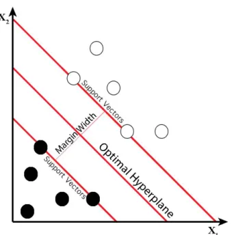
Fig. 1.Depiction of linearly separable binary class system. For visual-ization this figure depicts a two dimensional input space, while the input space for photo-zdetermination with SPIDERz is of higher dimension (the dimensions being all band magnitudes plus any other parameters). In this depiction the two classes are filled and open circles. The margin width is equal tokw2kwherewis a vector perpendicular to the hyperplane
as defined in Sect.2.2.
of support vector machine algorithms available in C++and Java (Chang & Lin 2011), modified with select customizations for optimization of photo-z estimation and implementation in the IDL environment. In addition to providing discrete redshift esti-mates for each galaxy, SPIDERz can also output photo-z prob-ability information (discussed below) and contains supplemen-tary programs for preprocessing galaxy inputs and performing data analysis.
Photo-zdetermination with SPIDERz, and indeed any ma-chine learning algorithm, consists of two main parts: training and evaluation. Inputs in the training process (the training set) are galaxy data consisting of band magnitudes, optional addi-tional parameters (morphological parameters in the case dis-cussed in this work), and known spectroscopic redshifts. The training process outputs a predictive model that can be applied to additional galaxy inputs (the evaluation set) in order to obtain photo-zestimates.
We link the galaxies in the training set to their known red-shift values by dividing them into redred-shift bins and assigning each a representative class label. Each galaxy and its correspond-ingnparameters (band magnitudes and potentially morphologi-cal parameters) are represented inn-dimensionalinput spaceas a galaxy input vector with n coordinates. The objective of the SVC training process is to construct a discriminative hyperplane that linearly separates galaxy vectors in the training set in such a way that maximizes the distance between galaxy vectors from opposing classes. Those vectors located closest to the separat-ing hyperplane are termed support vectors (SVs). For data sets with classes that are not linearly separable by an unbending hy-perplane in then-dimensional input space, as turns out to be the case in photo-zestimation and most practical scenarios, class separation requires the mapping of input vectors x from input space to a higherN-dimensionalfeature spacewith some func-tionφ:x 7→ φ(x). Once an optimal hyperplane solution for the
training set is obtained, unlabeled galaxy vectors (those in the evaluation set) are classified according to their location in fea-ture space with respect to the separating hyperplane.
For training a system withmdistinct classes (mredshift bins in this case), we use a so-called “one against one” or “pairwise coupling” approach (Hsu & Lin 2002;Knerr et al. 1990) that di-vides the multi-class system into a series of m(m2−1) separate bi-nary classification problems. The hyperplane optimization prob-lem is solved separately for each pair, and the unique hyperplane solutions (also called decision functions) are consolidated and collectively output as a predictive model. In the evaluation pro-cess, photo-z estimations are obtained by passing each galaxy vector in the evaluation set through the predictive model consist-ing of the m(m2−1)different binary classification problems solved in the training process. If a single-valued redshift prediction is desired, in the simplest implementation, which we employ in this work, the class to which a particular galaxy is most assigned be-comes its final predicted class (or redshift) value (or maximum probability value – see below).
To explore the algorithmic procedures for determining the decision hyperplane in such a binary classification case, let us picture a linearly separable binary class system like the one de-picted in Fig.1. Fori = 1, ...,l, each input vectorxi ∈ R2 has
an associated class labelyi ∈[−1,1], whereyi=1 for one class
of objects andyi = −1 for the other class of objects. The
opti-mal hyperplane is definted as asyi(w·xi+b) =0, wherewis
a vector perpendicular to the hyperplane andbis a scalar such that the distance from the origin to the hyperplane is k|bw|k. The following constraint is imposed on the support vectors (SVs), which are the data points located closest to the hyperplane in the space:
yi(w·xi+b)=1. (3)
It is important to note that the dot productw·xi is a distance
measure, and sincexiandyiare strictly defined, our SV
defini-tion is effectively specifying a scale forwandb. Working with these constraints, the decision function indicating the location of data points in this space can be stated as
yi(w·xi+b)≥1, (4)
which we can use to define a binary classifier for this system:
sgn(yi(w·xi+b)). (5)
Oncewis specified, this decision function is sufficient to classify objects in the linearly separable two class scheme. As previously discussed, the optimal hyperplane solution is the one in which the margin between SVs of opposing classes is maximized. The form of the decision function sets the width of the margin to
2
kwk, therefore our objective is to minimizekwk, or equivalently
1 2kwk
2. Finding an extremum of 1 2kwk
2subject to the constraints
imposed on the decision function presents a problem in the cal-culus of variations with a Lagrangian function
L(αi)= 1 2kwk 2−X i αi[yi(w·xi+b)−1] (6)
for which the minimizing conditions are given by the Euler-Lagrange equations. Following Cortes & Vapnik (1995) one finds
w=X
i
subject to the constraints (α i>0 for SVs αi=0 for non-SVs (8) X i αiyi=0. (9)
Thus wcan be expressed as a linear combination of SVs, and it’s clear that non-SVs are irrelevant to the optimal hyperplane solution. Finding the optimal hyperplane is now a matter of finding the correspondingαivalues for each SV that minimize
the Lagrangian of Eq. (6), now with the conditions in Eq. (7) inserted: L(αi)= 1 2 X i X j αiαjyiyjxi·xj− X i αi. (10)
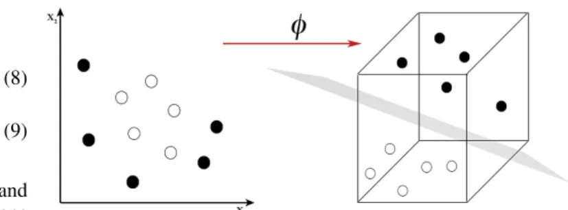
Let us now consider binary class systems that are not linearly separable in their original input space, like each of the m(m2−1) binary classification systems solved by SPIDERz. For such sys-tems, class separation requires mapping galaxy vectors x from ann-dimensional input space to a higherN-dimensional feature space with some functionφ:x 7→ φ(x). A visualization of such a mapping for a simplified scenario is presented in Fig.2. Since the Lagrangian stated in Eq. (10) depends on dot products of in-put vectors living in the same inin-put space, we represent the dot product of mapped vectors with a kernel function:
K(xi,xj)=φ(xi)·φ(xj). (11)
To solve for valid kernel functions that can successfully perform input vector dot products in N-dimensional feature space,Cortes & Vapnik(1995) applied Mercer’s theorem to the Hilbert-Schmidt theory concerning dot product expansions in Hilbert space, finding that one should use symmetric and pos-itive semi-definite kernel functions of the form:
K(xi,xj)=hφ(xi)|φ(xj)i (12)
or equivalently,
K(xi,xj)=φ(xi)T·φ(xj) (13)
where φ(xi)T ·φ(xj) is the inner product of the mapped
vec-tors. There are different variants of SVM kernels, however we obtained best results with the radial basis function (RBF) kernel
K(xi,xj)=e−γ||xi−xj||
2
, γ >0 (14)
whereγis a scaling factor of the distance measure between input vectorsxiandxjin theN-dimensional feature space, and whose
value is assigned before training. The RBF kernel, along with other kernels meeting conditions discovered byCortes & Vapnik
(1995), allows the mapping of dot products to feature space to be calculated without explicitly determining the functionφ. The free parameterγdetermines the topology of the decision surface in the feature space – a low value sets a geometrically compli-cated boundary while a high value sets a geometrically simpler one with greater potential for misclassifications.
Due to the size of the training set and number of galaxy characteristics contained in each training vector, it is not com-putationally practical to map the galaxy vectors to a feature space in such a way as to obtain a perfect linear separation between classes. Instead we employ a soft-margin approach
Fig. 2.Conceptual visualization of binary class system which is not lin-early separable in the input space (left) but is separable by a hyperplane when mapped to a higher dimensional feature space (right) with some functionφ:x7→φ(x).
(Cortes & Vapnik 1995) in which a prospective hyperplane so-lution is not required to inerrantly separate class values, but rather penalized for instances of misclassification during train-ing (mapped inputs falltrain-ing on the wrong side the separattrain-ing hy-perplane). This consideration is addressed with a cost function
fC=C
X
i
ξi, (15)
whereξi=0 if the training vector is correctly classified, and for
incorrectly classified training vectorsξiis the distance from the
misclassified point to the margin boundary described by the SVs of the correct class. The cost function is added as an additional term with additional constraints into the Lagrangian of Eq. (6):
L(αi, ξi)= 1 2kwk 2+CX i ξi− X i αi[yi(w·xi+b)−1+ξi]. (16)
The Euler-Lagrange equations then yield conditions that again allow the restatement of the Lagrangian as in Eq. (10) now with the additional constraint thatαi = C for the nonzeroαi. Thus
asCgets larger, a wider range of misclassifications are tolerated and the margin of class separation is larger, but those misclassi-fications that are not tolerated are penalized more.Cis therefore known as a “regularization parameter”.
The training process now requires the minimization of the Lagrangian of Eq. (10) constrained by
(α i=C for SVs αi=0 for non-SVs (17) X i αiyi=0. (18)
With the soft-margin approach, an optimal classifier is one that limits the number of misclassified input vectors while still max-imizing the distance from the separating hyperplane, with the relative importance of each factor having a dependence on the value ofC.
This optimization task is a so-called quadratic programming (QP) problem. Our training process solves the QP problem us-ing a decomposition method derived from Platt’s sequential min-imal optimization (Platt 1998), which tackles the problem by dividing it into multiple subproblems that can be analytically solved. For this we use the algorithmic solution described in
Chang & Lin(2011).
To obtain optimized values of the free parameters γandC
that allow the classifier to construct an optimal separating hyper-plane, SPIDERz conductsv-fold cross validation (CV) with a pa-rameter grid search. The CV process guards against over-fitting
the training set as well as approximates the performance of a pre-dictive model on an unknown evaluation set. CV randomly sep-arates training vectors intovsubsets of equal size, each of which sequentially serve as a pseudo-evaluation set for the predictive model created from a training set comprised of the remainingv -1 subsets. Rms error in redshift estimation is calculated during each iteration of CV and serves as the metric of predictive power of a model obtained from training with a particular combination ofC andγvalues. With a grid search that performs CV using every possible combination of allowedCandγvalues within a specified range and iterative step size, the program obtains opti-mal values ofCandγfor each training set by selecting the values associated with the lowest RMS error. To expedite runtime, we first perform a course grid search to identify a rough estimate of optimal parameters, and subsequently perform a fine grid search with a smaller parameter range and step size to achieve greater precision.
WithC,γ, and the SVs determined by training, we can ob-tain a predictive model (with m(m2−1) realizations corresponding to each binary pair of classes, as discussed above) and use it to estimate the photo-zs of galaxies in the evaluation set. For cal-culating the position of an evaluation vector relative to the sep-arating hyperplane, the kernel function is expressed in terms of support vectorssi
K(si,x)=e−γ||si−x||
2
, γ >0, (19)
and we can state a more precise formulation of the binary classi-fier introduced in Eq. (5):
sgn X
i
αiyiK(xs,xi)+b
. (20)
2.3. Redshift bins, probabilities, and single-valued photo-z estimates
Once them(m2−1)unique pairwise determinations betweenmbins of redshift have been made for a particular evaluation galaxy, the combination of these binary class estimates express what amounts to an effective probability distribution function (PDF) for each galaxy, with the relative probability of each bin propor-tional to the number of times the bin was chosen as the best bi-nary solution. This effective PDF is not continuous, but rather is resolved to the bin width level. Alternately, if one seeks a single value photo-zprediction for a galaxy, for reasons of efficiency, simplicity, or to determine performance metrics in a similar way to previous analyses, the most probable (commonly occurring) redshift bin result could be taken as a single valued photo-z esti-mate for the galaxy. For the purposes of the analyses in this work we focus on the later.
SPIDERz allows users flexibility in redshift bin size. We generally find determinations have increased accuracy and pre-cision when smaller bin sizes are used, however the optimal bin size for any determination will be dependent on the size and na-ture of the training set and can be approached via trial-and-error or approximated with the bin size introduced as an additional parameter in a grid search.
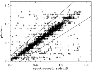
The top panel of Fig. 3 shows the estimated photo-z ver-sus spectroscopic redshift for the galaxies in the evaluation set of a particular determination with the AEGIS galaxy data set described in Sect.6with no morphological information in-cluded. This determination features 700 training galaxies and 1912 evaluation galaxies with a redshift bin size of 0.1. The
Fig. 3. Top: the estimated photo-zversus the actual redshift, as deter-mined by SPIDERz, for the AEGIS data set discussed in Sect.6with no morphological parameters included. The training set is formed from 700 galaxies and the evaluation set, for which the results are plotted, consists of the remaining 1912 galaxies. “Outliers” in a determination are defined by Eq. (1), shown as those outside of the two diagonal lines.
Middle: photo-zs for the same galaxies, as estimated with the custom
neural network as reported inSingal et al.(2011).Bottom: photo-zs for the same galaxies as estimated with the Lephare template fitting code
(Ilbert et al. 2006). The template fitting method has a lower scatter for
non-outliers, but a larger number of outliers than the SVM and neural network for these galaxies.
middle and bottom panel of Fig.3 also show photo-z estima-tions for the same training and evaluation galaxies with a cus-tom artificial neural network reported in Singal et al. (2011) and as evaluated with the Lephare template fitting method re-ported inIlbert et al. (2006). The SPIDERz determination ap-parently leads to fewer catastrophic outliers than with the Le-phare template fitting method or the neural network, although it shows a larger scatter among galaxies for which the
photo-z estimate is close to the actual redshift. It should be noted that template fitting methods such as LePhare, which consider template spectra evolved over a wide range of redshifts, are at
a potential disadvantage when estimating photo-zs in a limited redshift range relative to empirical methods where the redshift range of the training set would match that of the evaluation set, so it is not necessarily an indication of inferior performance that the LePhare determination has a comparatively higher number of catastrophic outliers (particularly at low spectroscopic redshifts) in this case.
3. Tests with the PHAT-1 catalog
In order to obtain a useful comparison with other photo-zcodes on publicly available data that spans a relatively large redshift range, we first focus on data available from the PHoto-z Accu-racy Testing (PHAT) program, which was implemented several years ago to test and compare photo-zcodes (Hildebrandt et al. 2010).
3.1. PHAT-1 dataset
At the time of the PHAT program, three spectroscopic and pho-tometric catalogs were assembled, with one (designated PHAT-1) based on real galaxy data. PHAT-1 featured a catalog of nearly 2000 galaxies with spectroscopic redshifts and 18-band photometry from the Great Observatories Origins Deep Survey (GOODS) North field. In the catalogs which were made avail-able, three-quarters of the spectroscopic redshifts, chosen at ran-dom, were “blinded” to the users with the intention that the users would utilize the other one-quarter as the training set and pre-dict the redshifts of the blinded galaxies, with results evaluated by the PHAT authors. As the PHAT program is no longer op-erational, we did not have the option of evaluating SPIDERz on the blinded galaxies. Therefore, we use only the unblinded galaxies, and to maintain the same proportions of training and evaluation galaxies as in the PHAT program, we use one-quarter (chosen at random) as the training set and the remaining three-quarters as the evaluation set. For a more straightforward eval-uation we also ignore galaxies with missing band magnitudes, which corresponds to the “cleaned sample” analysis reported in
Hildebrandt et al.(2010) and results in a set of 374 galaxies with known redshifts ranging from 0.08<z<3.6, and thus a training set with 94 galaxies and an evaluation set with 280 galaxies.
3.2. Results with PHAT-1 data
Even with this greatly reduced training set size our results on the PHAT-1 data are comparable to many other photo-zcodes. In Table 1 we show the results with SPIDERz along with those from other empirical codes as reported in Table 5 ofHildebrandt et al.
(2010). The other empirical codes reported there are the artificial neural network package ANNz (Collister & Lahav 2004), an em-piricalχ2 fitting code (Wolf 2009), a polynomial fit (Li & Yee 2008), and regression trees (Carliles et al. 2010). Results for the eight template fitting codes reported in that work vary from a high of 27.6% outliers and 0.061 reduced RMS to a low of 4.7% outliers and 0.038 reduced RMS. In Table 1 we also show results as reported for the two best-performing template fitting codes, LePhare (Ilbert et al. 2006) and BPz (Benítez 2000). Figure 4
shows the estimated photo-zversus actual redshift results of one particular determination with SPIDERz on the PHAT-1 dataset. We note that although the results from a full 18-band analysis are reported inHildebrandt et al.(2010), for a comparison anal-ysis with SPIDERz, we used only 17 bands in our determinations because of a large number of missing values in one band.
Fig. 4. Estimated photo-zas determined by SPIDERz versus the actual redshift for the PHAT-1 data set discussed in Sect.3.1for the case of 14 photometric bands. This determination is with a training set consist-ing of 94 galaxies chosen at random and an evaluation set consistconsist-ing of the other 280 galaxies. Outliers are defined by Eq. (1), shown as those outside of the two diagonal lines. This determination results in 15.3% outliers and a reduced RMS of 0.067, which, despite the smaller training set available, is competitive with the results obtained by other empirical methods as shown in Table 1 and discussed in Sect.3.2.
Table 1. Results for the “cleaned sample” of the PHAT-1 catalog with one-quarter of galaxies used for training and the remaining three-quarters used for evaluation, shown for SPIDERz as determined in this work along with other empirical codes and the two best performing tem-plate fitting codes as reported inHildebrandt et al.(2010).
14-band 18-band
Code Outlier % R-RMS Outlier % R-RMS
SPIDERz (0.1) 15.3 0.067 18.9 0.059 SPIDERz (0.2) 15.3 0.064 13.9 0.062 ANNz 36.5 0.078 29.0 0.074 χ2Emp. 13.3 0.066 15.3 0.067 Poly Fit 9.4 0.051 14.5 0.052 Regress. Trees 21.6 0.067 19.0 0.066 BPz 7.8 0.041 7.5 0.060 LePhare 4.7 0.038 4.9 0.040
Notes. Results for SPIDERz are shown for bin sizes of both 0.1 and 0.2 in redshift. Outliers are defined by Eq. (1) and the reduced RMS is given by Eq. (2) with outliers excluded. As discussed in Sect.3.1a much smaller training set was available for the SPIDERz determinations than was available for the others.
4. Tests with the COSMOS bright catalog
In order to obtain a data set with a large number of objects, and to investigate the effects of the inclusion of morphological information in photo-z determination, we turn to the COS-MOS field (e.g.Scoville et al. 2007), where multi-band photom-etry, spectroscopic redshifts, and morphological information are available for a large number of galaxies.
4.1. COSMOS bright data
In particular, we combine photometry from the COSMOS2015 photometric catalog (Laigle et al. 2016), the publicly available portion of the zCOSMOS catalog of spectroscopic redshifts (e.g.
Cassata et al. (2007). Using a 0.500 matching criterion for ob-jects, we obtain a catalog of 14 365 galaxies with photometry inu,B,V,r,i,z+,Y,H,J, andKs bands, seven morphological parameters, and spectroscopic redshifts rated as very secure. By construction all redshifts lie between 0 and 1.4.
Although the COSMOS2015 catalog provides photometry in a large number of optical, infrared, and UV bands, we choose to restrict our analyses to the bands listed above for several reasons. One reason is that outside of those bands the rate of missing pho-tometry is much higher. Another is that with data sets approach-ing 30 bands of photometry, the distinction between photo-z es-timation and spectroscopic redshift determination is somewhat muddled, and in any case this does not represent a realistic pho-tometric situation for upcoming large surveys such as LSST, even for subsets which would have infrared survey overlap.
The seven morphological parameters present in the catalog are
1. The Petrosian radiusRP: the mean radial distance from the
center of a galaxy at which the local intensity of the light equals some multiple η of the average intensity of light within the radius:I(RP)=η
RRP 0 I(r)2πrdr
πRP2
!
2. The half light radiusre: the radial distance from the center of
a galaxy within which half the total light is contained. 3. The concentrationc:c = 5 log r80
r20. This parameter defines
the central density of the light distribution with radiir80and
r20correspondingly 80% and 20% of the total light.
4. The asymmetryA:A=Σx,y|I(x,y)−I180(x,y)|
2Σx,y|Ix,y| −B180.This parameter characterizes the rotational symmetry of the galaxy’s light, withI(x,y)being the intensity at point (x, y) andI180(x,y)being
the intensity at the point rotated 180 degrees about the center from (x, y), with B180 being the average asymmetry of the
background calculated in the same way. It is the difference between object images rotated by 180◦.
5. The Gini coefficientG:
G=X n¯ (1n−1)Σ
n
i(2i−n−1)Xi, describes the uniformity of the
light distribution, withG =0 corresponding to the uniform distribution andG =1 to the case when all flux is concen-trated in to one pixel.Gis calculated by ordering all pixels by increasing fluxXi. ¯Xis a mean flux andnis the total number
of pixels.
6. M20: M20 = logΣMi/Mtot, is the ratio of the second order
moment of the brightest 20% of the galaxy to the total second moment. This parameter is sensitive to the presence of bright off-center clumps.
7. The axial ratio ε: ε = 1 − ba. The valuesa andb are the semi-major axis and semi-minor axis of the galaxy.
These parameters are discussed at greater length in e.g.
Scarlata et al.(2007).
4.2. Results with COSMOS bright data
We present several results with the COSMOS bright catalog. First we present results just utilizing the five optical bands u,
B,r,i, andz+, which could resemble the default situation for obtaining photometric redshifts from a very large optical survey. We also present results using these five optical bandsplus mor-phological parameters in order to explore whether the inclusion of morphological information can improve photo-zestimation in future large optical surveys. For completeness and comparison purposes we also present results utilizing all of the ten photo-metric bands listed above. Figure 5 shows a plot of estimated
Fig. 5. Estimated photo-zas determined by SPIDERz versus the actual redshift for the COSMOS data set discussed in Sect.4. This determi-nation was performed with ten-band photometry and a designated bin size of 0.01. The training and evaluation sets are comprised of 3000 and 11 365 randomly chosen galaxies, respectively. With this small bin size, a relatively large ratio of training set objects is needed in order to adequately bins with training objects. Outliers in a determination are defined by Eq. (1), shown as those outside of the two diagonal lines. The density of points within the lines is quite high – only 2.0% of points lie outside of the lines as outliers. This determination features a reduced RMS error of 0.022.
photo-zversus actual redshift for a particular determination in the ten-band case where we have used a small bin size of 0.01 as a demonstration.
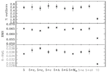
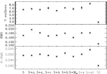
In order to quantify the variance for different determinations, we complete six realizations of training and evaluation for every case, each with a randomized training set of 1000 galaxies and an evaluation set of the remaining 13 365 galaxies, and record the number of outliers and RMS errors for the evaluation. Because the membership of the training and evaluation sets is random-ized, we obtain slightly varying numbers of outliers and RMS errors with each evaluation. Figure6shows the averaged number of outliers and RMS errors for determinations performed using five bands, five bands plus the inclusion of individual shape pa-rameters, five bands plus the inclusion of all shape papa-rameters, and lastly ten bands. We see that the inclusion of shape infor-mation does not result in a statistically significant improvement in the fraction of outliers, RMS, or reduced RMS as compared to the five-band only case. We discuss this further in Sect.7. As expected, estimates with the ten-band case are significantly bet-ter than with the five-band case. We also note that enlarging the training set size beyond 1000 galaxies for this data did not yield an appreciable improvement in either the fraction of outliers or the RMS errors when a binsize of 0.1 was used.
It is potentially interesting to compare the accuracy obtained with SPIDERz to that reported by the COSMOS collaboration’s own photo-zanalysis on similar data. With the former, in the ten-band case, we achieve an average of 1.8% outliers and an aver-age reduced RMS of 0.022. The numbers reported by the latter which most closely correspond to the former are from the “bright spectroscopic redshifts” sample reported by the COSMOS col-laboration inLaigle et al.(2016) where they achieve 0.5% out-liers and a reduced RMS of 0.007 with a method that is based on the LePhare (Ilbert et al. 2006) template fitting code. How-ever, it must be noted that the results inLaigle et al.(2016) are
Fig. 6.Percentage of outliers (top) along with non-reduced (middle) and reduced (bottom) RMS errorσ∆z/(1+z)in the photo-zestimation with the inclusion of different bands and morphological parameters in the COS-MOS field data set discussed in Sect.4as determined with SPIDERz. The uncertainties represent the standard deviation of the values obtained from different realizations featuring different random compositions of the training and evaluation sets, as discussed in Sect.4.2. Results are shown for the five-band case, the cases of five photometric bands plus each individual morphological parameter, the case of five photometric bands plus all morphological parameters, and the ten photometric band case.
obtained using up to 30 bands of photometry from ultraviolet to infrared including some quite narrow (<300 Å) bands. The two results then are difficult to compare directly, as the analysis with SPIDERz is disadvantaged by having fewer bands.
5. Tests with the COSMOS and 3D-HST overlap data
The COSMOS bright data set discussed in Sect.4 has the ad-vantage of containing many thousands of galaxies, but the dis-advantage of being limited to relatively low redshifts. To obtain a data set of real galaxies with publicly available spectroscopic redshifts that contains higher redshift sources we use spectro-scopic redshifts from the 3D-HST survey performed with the
HubbleSpace Telescope and reported inMomcheva et al.(2016) that overlap with COSMOS photometry and morphology. This results in a data set of 3048 galaxies, of which 206 (6.8%) have
z >2 and 537 (17.6%) havez>1.5. These galaxies have pho-tometry and morphological information as discussed in Sect.4.1. We note that this is the largest redshift range for which the inclu-sion of morphological information for photo-zdetermination has been tested, and that potentially morphological information may manifest an advantage in data sets with larger redshift ranges that is not present in narrower ranges.
As with the COSMOS bright data in Sect. 4.2, for the COSMOSx3D-HST data we present several results. First we present results just utilizing the five optical bands u, B, r, i, andz+, which could resemble the default situation for obtain-ing photometric redshifts from a very large optical survey. We also present results using these five optical bandsplus morpho-logical parameters in order to explore whether the inclusion of morphological information can improve photo-z estimation in future large optical surveys. For completeness and comparison purposes we also present results utilizing all of the ten photomet-ric bands listed above. Similarly, we complete six realizations of training and evaluation for every case, each with a random-ized training set of 1200 of the galaxies and an evaluation set of the remaining 1848 galaxies, and record the number of outliers
Fig. 7. Estimated photo-zas determined by SPIDERz versus the ac-tual redshift for the COSMOSx3D-HST data set discussed in Sect.5. This determination is with the ten-band photometric data and a training set consisting of 1200 galaxies chosen at random and an evaluation set consisting of the other 1848 galaxies, with a bin size of 0.1. Outliers in a determination are defined by Eq. (1), shown as those outside of the two diagonal lines. The density of points within the lines is quite high – only 2.6% of points lie outside of the lines as outliers. This determina-tion features a reduced RMS error of 0.04.
and the RMS errors for the redshift determination for the evalu-ation set. For this data we increase the proportion of training set galaxies in an effort to train the model with a greater represen-tation of the relatively scarce highest redshift population. Again, each randomized realization produces a slightly different number of outliers and RMS errors. Figure7shows a plot of estimated photo-zversus actual redshift for one particular determination in the ten-band case. Figure8shows the number of outliers and RMS errors for data sets composed of five bands, five bands plus the inclusion of individual shape parameters, five bands plus the inclusion of all shape parameters, and ten bands. We see again that the inclusion of shape information does not result in a statis-tically significant improvement in the fraction of outliers, RMS, or reduced RMS as compared to the five-band only case. As ex-pected, estimates with the ten-band case are significantly better than with the five-band case.
We note that SPIDERz performs remarkably well on this data set, including on the high redshift objects, considering that a small fraction of the galaxies are high redshift.
6. Tests with AEGIS data 6.1. AEGIS data
For comparison with previous results obtained with a neural network algorithm (Singal et al. 2011) we also perform tests on observations of the Extended Groth Strip from the the All-wavelength Extended Groth Strip International Survey (AEGIS) data set (Davis et al. 2007), which contains photometric band magnitudes inu,g,r,i, andzbands from the
Canada-France-Hawaii Telescope Legacy Survey (CFHTLS, Gwyn 2008),
imaging from the Advanced Camera for Surveys on the Hub-ble Space Telescope (HST/ACS, Koekemoer et al. 2007), and spectroscopic redshifts from the DEEP 2 survey using the DEIMOS spectrograph on the Keck telescope. The limiting i
band AB magnitude of the CFHTLS survey is 26.5, while that of HST/ACS is 28.75 inV(F606W) band, and that of DEEP2 is 24.1 inRband.
A total of 2612 galaxies spanning redshifts from 0.01 to 1.57, with a mean redshift of 0.702 and a median of 0.725, andiband magnitudes ranging from 24.43 to 17.62, are in the data set used here. The redshift distribution of this particular set of galaxies arises because of the intentional construction of the portion of DEEP2 spectroscopic catalog within the AEGIS survey to have roughly equal numbers of galaxies below and above z = 0.7; therefore it is not an optimized training set for a generic photo-metric data evaluation set, although a more optimized training set for any given photometric data evaluation set could be con-structed from it.
For shape information we use the following morpholog-ical parameters, previously derived in other works from the
HST/ACS imaging data in two bands, V (F606W) and I
(F814W):
1. The half light radiusre;
2. The concentrationc; 3. The asymmetryA; 4. The Gini coefficietG; 5. M20; and
6. The axial ratioε; all as defined in Sect.4.1, as well as 7. The smoothnessS:S =Σx,y|I(x,y)−IS(x,y)|
2Σx,y|Ix,y| −BS. The smoothness is
used to quantify the presence of small-scale structure in the galaxy. It is calculated by smoothing the image with a boxcar of a given width and then subtracting that from the original image. In this caseI(x,y) is the intensity at point (x, y) and
IS(x,y) is the smoothed intensity at (x, y), whileBS is the
av-erage smoothness of the background, calculated in the same way. The residual is a measure of the clumpiness due to fea-tures such as compact star clusters. In practice, the smooth-ing scale length is chosen to be a fraction of the Petrosian radius;
and
8. The Sérsic power law indexnswhere the Sérsic profile has a
formΣ(r) = Σee−k|(r/re) (1/ns )−1|
(e.g.Graham & Driver 2005), whereΣeis the surface brightness at radiusreandkis defined
such that half of the total flux is contained withinre.
Parameters c, A, S, G, and M20 are determined in Lotz et al.
(2008), whileε,ns, andreare determined byGriffith et al.(2012)
using the Galfit package (Peng et al. 2002;Häussler et al. 2007). For comparison with a previous result in this case we form principal components of the morphological parameters for this data set. Principal components (e.g.Jolliffe 2002) are the result of a coordinate rotation in a multi-dimensional space of possibly correlated data parameters into vectors with maximum orthogo-nal significance. The first principal component is along the direc-tion of maximum variadirec-tion in the data space, the second is along the direction of remaining maximum variation orthogonal to the first, the third is along the direction of remaining maximum vari-ation orthogonal to both of the first two, and so on. The morpho-logical principal components are given as linear combinations of the eight morphological parameters in Table 1 ofSingal et al.
(2011).
A further discussion of the particular mapping from mor-phological to principal components is available in Sect. 3 of
Singal et al.(2011). As mentioned there the first principal com-ponent is well correlated with galaxy type, and correlations per-sist through several of the other principal components. These correlations hinted that the morphology may provide an addi-tional handle on the photo-zestimation, since outliers often oc-cur because a spectral feature (such as a break) of one galaxy type at a given redshift may be seen by the observer to be at the
Fig. 8.Percentage of outliers (top) along with non-reduced (middle) and reduced (bottom) RMS errorσ∆z/(1+z)in the photo-zestimation with the inclusion of different bands and morphological parameters in the COSMOSx3D-HST data set discussed in Sect.5as determined with SPIDERz. The uncertainties represent the standard deviation of the val-ues obtained from different realizations featuring different random com-positions of the training and evaluation sets, as discussed in Sect.4.2. Results are shown for the five photometric band case, the cases of five photometric bands plus each individual morphological parameter, the case of five photometric bands plus all morphological parameters, and the ten photometric band case.
same wavelengths as a spectral feature of another galaxy type at different redshift. Thus it was an intriguing hypothesis that morphological information indicative of galaxy type may help break this degeneracy.
6.2. Results with AEGIS data
As in Sects.4.2and5 we complete six realizations of training and evaluation for every case, for this data with a randomized training set of 700 of the galaxies discussed in Sect. 6.1 and an evaluation set of the remaining 1912 galaxies, and record the number of outliers and the RMS error for the redshift de-termination for the evaluation set. Here as well because in each realization the membership of the training and evaluation sets varies, each realization for a given input parameter set produces a slightly different number of galaxies in the evaluation set that are outliers and a slightly different RMS error. For comparison, the template fitting results reported byIlbert et al.(2006) using band photometry only give 5% outliers and a (non-reduced) RMS er-ror ofσ∆z/(1+z) =.1881 for this sample. This error is dominated
by the catastrophic outliers (Fig.3), and clearly visually drops to below that of SPIDERz if outliers are excluded.
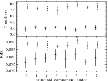
Figure 9 shows the number of outliers and RMS error for the inclusion of the seven different principal components indi-vidually. Figure10shows the number of outliers and RMS error for the inclusion of multiple principal components, starting with none, then adding in the first, then adding in the first and second, then adding in the first through third, and so on. We do not show the reduced RMS in this case because it is not available for com-parison in the neural network determination. In each figure, the error bars correspond to the standard deviation of the number of outliers or RMS scatter in the different realizations. We note that the last principal component (PC8) should by definition contain minimal significant variation in the morphological parameters, so we do not include it in the analysis.
Fig. 9.Percentage of outliers (top) and non-reduced RMS errorσ∆z/(1+z) (bottom) in the photo-z estimation with the inclusion of different in-dividual principal components of the morphological parameters with the AEGIS data set discussed in Sect. 6, shown for SPIDERz (solid lines and star points) and for the custom neural network described in
Singal et al. (2011; dashed lines and cross points). The uncertainties
represent the standard deviation of the values obtained from different realizations featuring different compositions of the training and evalua-tion sets, as discussed in Sect.6.2.
Fig. 10. Percentage of outliers (top) and non-reduced RMS error
σ∆z/(1+z)(bottom) in the photo-zestimation with the inclusion of mul-tiple principal components of the morphological parameters with the AEGIS data set discussed in Sect.6, starting with none, adding the first morphological principal component, then the first and the second prin-cipal components, and so on. Results are shown for SPIDERz (solid lines and star points) and for the custom neural network described in
Singal et al. (2011, dashed lines and cross points). The uncertainties
represent the standard deviation of the values obtained from different realizations featuring different compositions of the training and evalua-tion sets, as discussed in Sect.6.2.
It is apparent that the SVM algorithm of SPIDERz results in a significant decrease in the number of outliers and RMS error compared to the artificial neural network algorithm pre-viously tested. In addition, the standard deviation for diff er-ent realizations in the number of outliers is generally smaller
with the SVM method, allowing us to determine that adding morphological information in the form of individual principal components of the morphological parameters does not provide a statistically significant decrease in the average number of out-liers or the RMS error, while adding multiple principal compo-nents increases the number of outliers and the RMS error.
7. Discussion
We have developed a custom SVM classification algorithm for photometric redshift estimation in the IDL environment. The package, SPIDERz, is available to the community. It outputs for each galaxy both an effective distribution of probabilities (in bins of redshift) for each galaxy’s photo-zand a single-valued, most likely predicted photo-zbin, with the bin size chosen by the user. In this analysis for practicality of evaluating metrics such as outliers and RMS errors we use only the single-valued photo-z
prediction.
We compare results obtained with SPIDERz to those pre-viously reported for other codes with the PHAT-1 catalog in Sect.3.2. We see that SPIDERz performs comparable to other empirical methods on this catalog, noting that as discussed in Sect.3.1far fewer training galaxies were available for SPIDERz. On this latter point, having such a reduced number of training galaxies available is a significant disadvantage for SPIDERz or any empirical method in a dataset such as PHAT-1 where pro-portionally few of the galaxies are higher redshift. In the context of SVC as discussed in Sect.2.2, as the training data in certain redshift bins becomes sparse, there may be insufficient support vectors available for those bins in the binary classifications for effective hyperplane solutions.
SPIDERz can naturally include additional parameters be-yond band magnitudes. We note that an SVM is in a sense an unbiased way of determining the relative strength of the corre-lations of a set of input parameters with the output parameter, and that this SVM algorithm is designed to treat all input pa-rameters on an equal footing, thus providing for a convenient method for investigating the inclusion of additional inputs be-yond photometry.
In order to both explore a much larger dataset and exam-ine the effects of the inclusion of morphological parameters on photo-zestimation, we form a data set of 14 365 galaxies with photometry, morphological parameters, and spectroscopic red-shifts from the COSMOS field as discussed in Sect.4. We find that while SPIDERz performs relatively well on this data, that the inclusion of morphological information in the form of mor-phological parameters does not improve the number of outliers or RMS errors in photo-zestimation over the case of five opti-cal photometric bands only. As expected, using ten photometric bands reduces the number of outliers and RMS errors consider-ably relative to five bands.
To study the performance of SPIDERz and the effects of in-cluding morphological parameters over a larger redshift range we form a data set of 3048 galaxies from the overlap of COS-MOS photometry and morphology with 3D-HST spectra as dis-cussed in Sect.5. We find SPIDERz performs quite well on this data, including on higher redshift galaxies, even though these galaxies form a small fraction of the training set. We again find that the inclusion of morphological information in the form of morphological parameters does not improve the number of out-liers or RMS errors in photo-zestimation over the case of five optical photometric bands only, and again using ten photometric
bands reduces the number of outliers and RMS errors consider-ably relative to five bands.
For comparison with a previous determination with a neural network algorithm, we also estimate photo-zfor a data set which consists of 2612 galaxies with five optical band magnitudes, re-liable spectroscopic redshifts, and principal components of eight morphological parameters, discussed in Sect.6. We again find that the inclusion of morphological information does not signif-icantly decrease the number of outliers or RMS error in photo-z
estimation. PreviouslySingal et al.(2011) found compatible re-sults with the neural network estimation method. We do note that the inclusion of multiple principal components resulted in a diminished performance in photo-zestimation with the neural network algorithm due to the addition of noise while this had less of an effect on the performance of SPIDERz, indicating that per-haps SVMs are less susceptible to the negative effects of adding noise in this situation.
The particular findings regarding the inclusion of shape in-formation thus evidence some robustness in regard to different data sets, consideration of morphological parameters or princi-pal components, and consideration of an SVM or neural network method. We conclude, therefore, that these results are likely ap-plicable to all empirical methods with this redshift range and photometry restricted to the visible and near infrared bands. Any gain that may arise in an empirical photo-zdetermination from correlations between morphology and redshift is overwhelmed by the additional noise introduced. It is likely that any corre-lations between the morphological parameters and the galaxy type are degenerate to some extent with the correlations between galaxy type and galaxy colors. The possibility remains that un-der a less input-blind and more complicated scenario where, for example, the regularization parameter for misclassification (see Eq. (15)) varies with the redshift, the additional noise con-tained in morphological information could be made less conse-quential. A potentially more straightforward possibility is that morphological information along with probability distribution considerations could be used only to flag galaxies more likely to be catastrophic outliers, which we will explore in a future work.
Acknowledgements. The authors acknowledge data supplied previously by B. Gerke, M. Shmakova, R.L. Griffith, and J. Lotz. Based in part on observations made with the NASA/ESAHubbleSpace Telescope, obtained from the Data Archive at the Space Telescope Science Institute, which is operated by the As-sociation of Universities for Research in Astronomy, Inc., under NASA contract NAS 5-26555. Funding for the DEEP2 survey has been provided by NSF grants AST-0071048, AST-0071198, AST-0507428, and AST-0507483. Some of The data presented herein were obtained at the W. M. Keck Observatory, which is operated as a scientific partnership among the California Institute of Technology, the University of California and the National Aeronautics and Space Adminis-tration. The Observatory was made possible by the generous financial support of the W. M. Keck Foundation. The DEEP2 team and Keck Observatory acknowl-edge the very significant cultural role and reverence that the summit of Mauna Kea has always had within the indigenous Hawaiian community and appreciate the opportunity to conduct observations from this mountain.
References
Arnouts, S., Cristiani, S., Moscardini, L., et al. 1999,MNRAS, 310, 540
Beaumont., C., Williams, J., & Goodman, A. 2011,ApJ, 741, 14
Benítez, N. 2000,ApJ, 536, 571
Burges, C. 1998,Data Mining and Know Disc, 2, 2
Budavari, T., Szalay, A. S., Charlot, S., et al. 2005,ApJ, 619, L31
Carrasco Kind, M., & Brunner, R. 2013,MNRAS, 432, 2
Carliles, S., Budavari, T., Heinis, S., Priebe, C., & Szalay, A. S. 2010,ApJ, 712, 511
Cassata, P., Guzzo, L., Franceschini, A., et al. 2007,ApJS, 172, 270
Chang, C., & Lin, C. 2011,LIBSVM: a library for support vector machines, ACM Transactions on Intelligent Systems and Technology, 2, 1
Collister, A., & Lahav, O. 2004,PASP, 116, 345
Cortes, C., & Vapnik, V. 1995,Machine Learning, 20, 3
Davis, M., Guhathakurta, P., Konidaris, N. P., et al. 2007,ApJ, 660, L1
Gerdes, D., Sypniewski, A. J., McKay, T. A., et al. 2010,ApJ, 715, 823
Graham, A., & Driver, S. 2005,PASA, 22, 118
Griffith, R., Cooper, M. C., Newman, J. A., et al. 2012,ApJS, 200, 9
Gwyn, S. 2008,PASP, 120, 212
Hassan., T., Mirabal, N., Contreras, J., & Oya, L. 2013,MNRAS, 428, 220
Häussler, B., McIntosh, D. H., Barden, M., et al. 2007,ApJS, 172, 615
Haykin, S. 1999, Neural Networks: A Comprehensive Foundation, Upper Saddle River (NJ: Prentice Hall)
Hearin, A., Zentner, A., Ma, Z., & Huterer, D. 2010,ApJ, 720, 135
Hearst, M., Scholköpf, B., Dumais, S., Osuna, E., & Platt, J. 1998,IEEE Int. Syst, 13, 18
Hildebrandt, H., Arnouts, S., Capak, P., et al. 2010,A&A, 523, A31
Huretas-Company, M., Tasca, L., Rouan, D., et al. 2008,A&A, 497, 743
Hsu, C.-W., & Lin, C.-J. 2002,IEEE Trans Neural Net, 13, 2
Huterer, D., Takada, M., Bernstein, G., & Jain, B. 2006,MNRAS, 366, 101
Ilbert, O., Arnouts, S., McCracken, H. J., et al. 2006,A&A, 457, 841
Ivezic, Z., Tyson, J. A., Abel, B., et al. 2008, ArXiv e-prints [arXiv:0805.2366]
Jolliffe, I. 2002, Principal Component Analysis. Series: Springer Series in Statistics, 2nd edn. (New York: Springer)
Klement, R. J., Bailer-Jones, C. A. L., Fuchs, B., Rix, H.-W., & Smith, K. W. 2011,ApJ, 726, 103
Knerr, S., Personnaz, L., & Dreyfyus, G. 1990, in Neurocomputing: Algorithms, Architectures, and Applications (Springer)
Koekemoer, A., Aussel, H., Calzetti, D., et al. 2007,ApJS, 172, 196
Laigle, C., McCracken, H. J., Ilbert, O., et al. 2016,ApJS, 224, 24
Lilly, S., Le Brun, V., Maier, C., et al. 2009,ApJS, 184, 218
Li, I., & Yee, H. 2008,AJ, 135, 809
Lotz, J. M., Davis, M., Faber, S. M., et al. 2008,ApJ, 672, 177
Malek, K., Solarz, A., Pollo, A., et al. 2013,A&A, 557, A16
Marton, G., Toth, L., Paladini, M., et al. 2016,MNRAS, 458, 347
Momcheva, I. G., Brammer, G. B., van Dokkum, P. G., et al. 2016,ApJS, 225, 27
Peng, C., Ho, L., Impev, C., & Rix, H. 2002,AJ, 124, 266
Platt, J. 1998, Microsoft Technical Report, MSR-TR-98-14 Scarlata, C., Carollo, C. M., Lilly, S., et al. 2007,ApJS, 172, 406
Scoville, A., Aussel, H., Brusa, M., et al. 2007,ApJS, 172, 1
Singal, J., Shmakova, M., Gerke, B., Griffith, R. L., & Lotz, J. 2011,PASP, 123, 615
Solarz, A., Pollo, A., Takeuchi, T. T., et al. 2012,A&A, 541, A50
Tagliaferri, R., Longo, G., Andreon, S., et al. 2003,Lect. Notes Comp. Sci., 2859, 226
Vanzella, E., Cristiani, S., Fontana, A., et al. 2004,A&A, 423, 761
Vince, O., & Csabai, I. 2007,Toward more precise photometric redshift estima-tion, Proc. International Astronomical Union, 241, 573
Wadadekar, Y. 2004,PASP, 117, 79
Wang, D., Zhang, Y., Liu, C., & Zhao, Y. 2007,CJAA, 7, 43
Way, M., & Srivastava, A. 2006,ApJ, 647, 102