Building an Efficient RDF Store Over a Relational Database

Building an Efficient RDF Store Over a Relational Database

Mihaela A. Bornea

, Julian Dolby

, Anastasios Kementsietsidis

Kavitha Srinivas

, Patrick Dantressangle

, Octavian Udrea

, Bishwaranjan Bhattacharjee

IBM Research

{

_mbornea,

_dolby,

_akement,

_ksrinivs,

_oudrea,

_{bhatta}@us.ibm.com,}

_{[email protected]}

ABSTRACT

Efficient storage and querying of RDF data is of increasing impor-tance, due to the increased popularity and widespread acceptance of RDF on the web and in the enterprise. In this paper, we describe a novel storage and query mechanism for RDF which works on top of existing relational representations. Reliance on relational repre-sentations of RDF means that one can take advantage of 35+ years of research on efficient storage and querying, industrial-strength transaction support, locking, security, etc. However, there are sig-nificant challenges in storing RDF in relational, which include data sparsity and schema variability. We describe novel mechanisms to shred RDF into relational, and novel query translation tech-niques to maximize the advantages of this shredded representation. We show that these mechanisms result in consistently good per-formance across multiple RDF benchmarks, even when compared with current state-of-the-art stores. This work provides the basis for RDF support in DB2 v.10.1.

Categories and Subject Descriptors

H.2 [Database Management]: Systems

Keywords

RDF; Efficient Storage; SPARQL; Query optimization

1.

INTRODUCTION

While the Resource Description Framework (RDF) [14] format is gaining widespread acceptance (e.g.,Best Buy [3], New York Times [18]), efficient management ofRDFdata is still an open prob-lem. In this paper, we focus on two aspects of efficiency, namely, storage and query evaluation. Proposals for storage ofRDFdata can be classified into two categories, namely,Nativestores (e.g.,Jena TDB [23], RDF-3X [13], 4store [1]) which use customized binary RDFdata representations, andRelationally-backedstores (e.g.,Jena SDB [23], C-store [2]) which shredRDFdata to appropriate rela-tional tables. While there is evidence that going native pays in terms of efficiency, we cannot completely disregard relationally-backed stores. For one thing, relational stores come with 35+ years

Permission to make digital or hard copies of all or part of this work for personal or classroom use is granted without fee provided that copies are not made or distributed for profit or commercial advantage and that copies bear this notice and the full citation on the first page. To copy otherwise, to republish, to post on servers or to redistribute to lists, requires prior specific permission and/or a fee.

SIGMOD’13,June 22–27, 2013, New York, New York, USA. Copyright 2013 ACM 978-1-4503-2037-5/13/06 ...$15.00.

of research on efficient storage and querying. More importantly, relational-backed stores offer important features that are mostly lacking from native stores, namely, scalability, industrial-strength transaction support, compression, security, to name a few. How-ever, there are important challenges in using a relational database as anRDFstore, the most important of which stem from the inherent mismatch between the relational andRDFmodels. DynamicRDF schemas and data sparsity are typical characteristics ofRDFdata which are not commonly associated with relational databases. So, it is not a coincidence that existing approaches that storeRDFdata over relational stores [2,21,23] cannot handle this dynamicity with-out altering their schemas. More importantly, existing approaches cannot scale to largeRDFstores and cannot handle efficiently many complex queries. Our first contribution is an innovative relational storage representation forRDFdata that is both flexible (it does not require schema changes to handle dynamicRDFschemas), and scal-able (it handles efficiently the most complex queries).

Efficient querying is our next contribution, with the query lan-guage of choice inRDF currently beingSPARQL[16]. Although there is a large body of work in query optimization (both in SPARQL[8,11,13,17,19] and beyond), there are still important chal-lenges in terms of (a)SPARQLquery optimization, and (b) trans-lation ofSPARQL to equivalentSQLqueries. Typical approaches perform bottom-up SPARQL query optimization, i.e., individual triples [17] or conjunctiveSPARQLpatterns [13] are independently optimized, and then the optimizer orders and merges these indi-vidual plans into one global plan. These approaches are similar to typical relational optimizers which rely on statistics to assign costs to query plans (in contrast to approaches [19] where statis-tics are ignored). While these approaches are adequate for sim-ple SPARQL queries, they are not as effective for more compli-cated, but still common, SPARQLqueries, as we illustrate in this paper. Such queries often have deep, nested sub-queries whose inter-relationships are lost when optimizations are limited by the scope of single triple or individual conjunctive patterns. To address such limitations, we introduce a hybrid two-step approach to query optimization. As a first step, we construct a specialized structure, called a data flow, that captures the inherent inter-relationships due to the sharing of common variables or constants of different query components. These inter-relationships often span the boundaries of simple conjuncts (or disjuncts) and are often across the differ-ent levels of nesting of a query,i.e.,they are not visible to existing bottom-up optimizers. As a second step, we use the data flow and cost estimates to decide both the order with which to optimize the different query components, and the plans we are to consider.

While our hybrid optimizer searches for optimal plans, this search must be qualified by the fact that ourSPARQLqueries must be converted toSQL. That is, our plans should be such that when they

are implemented inSQL, they are (a) amenable to optimizations by the relational query engine; and (b) can be efficiently evaluated in the underlying relational store. So in our setting,SPARQLacts as a declarative query language that is optimized, whileSQLbecomes a procedural implementation language for our plans. This depen-dence onSQL essentially transforms our problem from a purely query optimization problem into a combined query optimization and translation problem. The translation part is particularly com-plex since there are many equivalentSQLqueries that implement the sameSPARQLquery plan. Consistently finding the rightSQL query is one of the key challenges and contributions of our work.

Note that both the hybrid optimization and the efficientSPARQL -to-SQL translation are contributions that are not specific to our work, and both techniques are generalizable and can be applied in anySPARQLquery evaluation system. So our hybrid optimizer can be used forSPARQLquery optimization, independent of the se-lectedRDFstorage (with or without a relational back-end); our ef-ficient translation ofSPARQLtoSQLcan be generalized and used for any relational storage configuration ofRDF(not just the one we introduce here). The combined effects of these two independent contributions drive the performance of our system.

The effectiveness of both our optimizer and our relational back-end are illustrated through detailed experiments. There has been lots of discussion [6, 9] as to what is a representativeRDFdataset (and associated query workload) for performance evaluation. Dif-ferent papers have used difDif-ferent datasets with no clear way to cor-relate results across works. To provide a thorough picture of the current state-of-the-art, and illustrate the novelty of our techniques, we provide as our last contribution an experimental study that con-trasts the performance offivesystems (including ours) againstfour different (real and benchmark) data sets. Our work provides the basis for RDF support in DB2 v.10.1.

2.

RDF OVER RELATIONAL

There have been many attempts to shredRDFdata into the rela-tional model. One approach involves a singletriple-storerelation with three columns, for the subject, predicate and object. Then, eachRDFtriple becomes a single tuple, which for a popular dataset like DBpedia results in a relation with 333M tuples (one perRDF triple). Figure 1(a) shows a sample of DBpedia data, used as our running example. The triple-store can deal with dynamic schemas since triples can be inserted without a priori knowledge ofRDF data types. However, efficient querying requires specialized tech-niques [13]. A second alternative is atype-orientedapproach [23] where one relation is created for eachRDFdata type. So, for our data in Figure 1(a), we create one relation for people (e.g.,to store

Charles Flinttriples) and another for companies (e.g.,to storeGoogle

triples). Dynamic schemas require schema changes as newRDF types are encountered, and the number of relations can quickly get out of hand if one considers that DBpedia includes 150K types. Finally, a third alternative [2, 21] considers apredicate-oriented approach centered around column-stores where a binary subject-object relation is created for each predicate. So, in our example, we create one relation for theborn, one for thediedpredicate etc. Similar to the type-oriented approach, dynamic schemas are prob-lematic as new predicates result in new relations, and in a dataset like DBpedia these can number in the thousands. In what follows, we introduce a fourthentity-orientedalternative which avoids both the skinny relation of the first approach, and the schema changes (and thousands of relations) required by the latter two.

2.1

The

schema

The triple-store offers flexibility in the tuple dimension since new triples irrespectively of type or predicate are added to the rela-tion. The intuition behind our entity-oriented approach is to carry this flexibility in the column dimension. Specifically, the lesson learned from the latter two alternatives is that there is value in stor-ing objects of the same predicate in the same column. So, we in-troduce a mechanism in which we treat the columns of a relation as flexible storage locations that are not pre-assigned to any predicate, but predicates are assigned to themdynamically, during insertion. The assignment ensures that a predicate is always assigned to the same column or more generally the same set of columns.

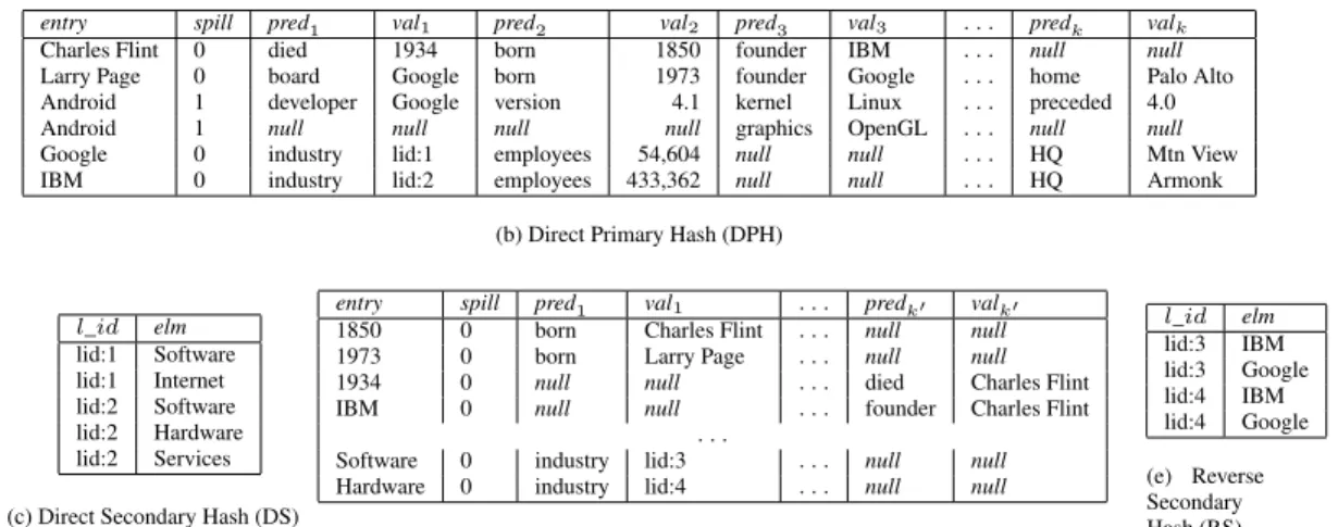
We describe the basic components ofDB2RDFschema in Fig-ure 1. TheDirect Primary Hash (DPH)(shown in Figure 1(b) and populated with the data from Figure 1(a)) is the main relation in the schema. Briefly, DPH is a wide relation in which each tuple stores a subjectsin theentrycolumn, with all its associated predicates and objects stored in theprediandvalicolumns0 ≤i ≤k,

respec-tively. If subjectshas more thankpredicates,i.e.,|pred(s)|> k, then((|pred(s)|/k) + 1)tuples are used fors,i.e.,the first tuple stores the firstkpredicates fors, andsspills(indicated by thespill column) into a second tuple and the process continues until all the predicates forsare stored. For example, all triples forCharles Flintin Figure 1(a) are stored in the first DPH tuple, while the second DPH tuple stores allLarry Pagetriples. Assuming more thankpredicates forAndroid, the third DPH tuple stores the firstkpredicates while extra predicates, likegraphics, spill into the fourth DPH tuple.

Multi-valued predicates require special treatment since their multi-values (objects) cannot fit into a singlevalicolumn.

There-fore, we introduce a second relation, called theDirect Secondary Hash (DS). When storing a multi-valued predicate in DPH, a new unique identifier is assigned as the value of the predicate. Then, the identifier is stored in the DS relation and is associated with each of predicate values. To illustrate, in Figures 1(b) and (c), theindustry

forGoogleis associated with lid:1 in DPH, while lid:1 is associated in the DS relation with object valuesSoftwareandInternet.

Note that although a predicate is always assigned to the same column (for any subject having this predicate), the same column stores multiple predicates. So, we assign the founderpredicate to column pred₃ for both theCharles Flint and the Larry Pagesubjects, but the same column is also assigned to predicates likekerneland

graphics. Having all the instances of a predicate in the same column provides us with all the advantages of traditional relational repre-sentations (i.e.,each column stores data of the same type) which are also present in the type-oriented and predicate-oriented repre-sentations. Storing different predicates in the same column leads to significant space savings since otherwise we would require as many columns as predicates in the data set. In this manner, we use a rel-atively small number of physical columns to store datasets with a much larger number of predicates. This is also consistent with the fact that although a dataset might have a large number of predicates, not all subjects instantiate all predicates. So, in our sample dataset, the predicatebornis only associated with subjects corresponding to humans, likeLarry Page, while thefoundedpredicate is associated only with companies. Of course, a key question is how exactly we do this assignment of predicates to columns and how we decide this valuek. We answer this question in Section 2.2 and also provide evidence that this idea actually works in practice.

From anRDFgraph perspective, the DPH and DS relations essen-tially encode the outgoing edges of an entity (the predicatesfrom a subject). For efficient access, it is advantageous to also encode the incoming edges of an entity (the predicatestoan object). To this end, we provide two additional relations, called the Reverse

(Charles Flint, born, 1850) (Charles Flint, died, 1934) (Charles Flint, founder, IBM) (Larry Page, born, 1973) (Larry Page, founder, Google) (Larry Page, board, Google) (Larry Page, home, Palo Alto) (Android, developer, Google) (Android, version, 4.1) (Android, kernel, Linux) (Android, preceded, 4.0)

. . .

(Android, graphics, OpenGL) (Google, industry, Software) (Google, industry, Internet) (Google, employees, 54,604) (Google, HQ, Mountain View) (IBM, industry, Software) (IBM, industry, Hardware) (IBM, industry, Services) (IBM, employees, 433,362) (IBM, HQ, Armonk) (a) Sample DBpedia data

entry spill pred₁ val1 pred2 val2 pred3 val3 . . . predk valk

Charles Flint 0 died 1934 born 1850 founder IBM . . . null null

Larry Page 0 board Google born 1973 founder Google . . . home Palo Alto Android 1 developer Google version 4.1 kernel Linux . . . preceded 4.0 Android 1 null null null null graphics OpenGL . . . null null

Google 0 industry lid:1 employees 54,604 null null . . . HQ Mtn View IBM 0 industry lid:2 employees 433,362 null null . . . HQ Armonk

(b) Direct Primary Hash (DPH)

l_id elm lid:1 Software lid:1 Internet lid:2 Software lid:2 Hardware lid:2 Services

(c) Direct Secondary Hash (DS)

entry spill pred₁ val1 . . . predk0 valk0

1850 0 born Charles Flint . . . null null

1973 0 born Larry Page . . . null null

1934 0 null null . . . died Charles Flint IBM 0 null null . . . founder Charles Flint

. . .

Software 0 industry lid:3 . . . null null

Hardware 0 industry lid:4 . . . null null

(d) Reverse Primary Hash (RPH)

l_id elm lid:3 IBM lid:3 Google lid:4 IBM lid:4 Google (e) Reverse Secondary Hash (RS)

Figure 1: Sample DBpedia RDF data and the correspondingDB2RDFschema

Predicate Set Freq.

SV1SV2SV3SV4 _.01 MV1MV2MV3MV4 SV1SV2SV3 _.24 MV1MV2MV3 SV1SV3SV4 _.25 MV1MV3MV4 SV2SV3SV4 _.25 MV2MV3MV4 SV1SV2SV4 _.24 MV1MV2MV4 SV5SV6SV7SV8 .01 Table 1: Micro-Bench Characteristics

Query Star query predicate set Results Q1 SV1SV2SV3SV4 938 Q2 MV2MV2MV3MV4 10313 Q3 SV1 10313 MV1MV2MV3MV4 Q4 SV1SV2 ₁₀₃₁₃ MV1MV2MV3MV4 Q5 SV1SV2SV3 10313 MV1MV2MV3MV4 Q6 SV1SV2SV3SV4 10313 MV1MV2MV3MV4 Q7 SV5 2500 Q8 SV5SV6 2500 Q9 SV5SV6SV7 2500 Q10 SV5SV6SV7SV8 2500

Table 2: Micro-Bench Queries Primary Hash (RPH)and theReverse Secondary Hash (RS), with samples shown in Figures 1(d) and (e).

Advantages of

Layout.

An advantage of theDB2RDFschema is the elimination of joins in star queries (i.e., queries that ask for multiple predicates for the same subject or object). Star queries are quite common inSPARQL workloads, and complexSPARQLqueries frequently contain sub-graphs that are stars. Star queries can involve purely single valued predicates, purely multi-valued predicates, or a mix of both. While for single valued predicates theDB2RDFlayout reduces star query processing to a single row lookup in the DPH relation, processing of multi-valued or mixed stars requires additional joins with DS relation. It is unclear how these additional joins impact the perfor-mance ofDB2RDFwhen compared to the other types of storage.

To this end, we designed a micro benchmark that contrasts query processing inDB2RDFwith the triple-store and predicate-oriented approaches1. The benchmark has 1MRDF triples with the char-acteristics defined in Table 1. Each table row represents a predi-cate set along with its relative frequency distribution in the data. So, subjects with the predicate set {SV1, SV2, SV3, SV4, MV1, MV2,MV3,MV4}(first table row) constituted 1% of the 1 million dataset. The predicatesSV1toSV8were all single valued, whereas MV1 toMV4 were multi-valued. The predicate sets are such that a single valued star query forSV1,SV2,SV3andSV4is highly se-lectivebut only when all four predicates are involved in the query.

1_{We omitted the type-oriented approach because for this micro-benchmark it is similar}

to the entity-oriented approach.

SELECT ?sWHERE{?sSV₁?o1.?sSV₂?o2.?sSV₃?o3.?sSV₄?o4}

(a) SPARQL for Q1

SELECT T.entryFROMDPH AS T

WHERE T.PRED0=’SV₁’ANDT.PRED1=’SV₂’ANDT.PRED2=’SV₃’ANDT.PRED3=’SV₄’ (b) Entity-oriented SQL

SELECT T1.SUBJFROMTRIPLE AS T1, TRIPLE AS T2, TRIPLE AS T3, TRIPLE AS T4

WHERE T1.PRED=’SV₁’ANDT2.PRED=’SV₂’ANDT3.PRED=’SV₃’ANDT4.PRED=’SV₄’AND

T1.SUBJ = T2.SUBJANDT2.SUBJ = T3.SUBJANDT3.SUBJ = T4.SUBJ (c) Triple-store SQL

SELECT SV1.ENTRYFROMCOL_SV₁AS SV1, COL_SV₂AS SV2, COL_SV₃AS SV3, COL_SV₄AS SV4

WHERE SV1.ENTRY = SV2.ENTRYANDSV2.ENTRY = SV3.ENTRYANDSV3.ENTRY = SV4.ENTRY (d) Predicate-oriented SQL

Figure 2: SPARQL and SQL queries for Q1

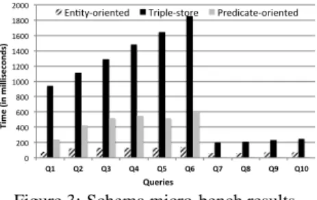
The predicates by themselves are not selective. Similarly, a multi-valued star query forMV1,MV2,MV3 andMV4 is selective, but only if it involves all four predicates. We also consider a set of se-lective single valued predicates (SV5toSV8) to separately examine the effects of changing the size of a highly selective single valued star on query processing, while keeping the result set size constant. Table 2 shows the predicate sets used to construct star queries. Figure 2(a) shows theSPARQLstar query corresponding to the pred-icate set for Q1 in Table 2. For each constructedSPARQLquery, we generated threeSQLqueries, one for each of theDB2RDF, triple-store, and predicate-oriented approaches (see Figure 2 for theSQL queries corresponding to Q1). In all three cases, we only index subjects, since the queries only join subjects. Q1 examines sin-gle valued star query processing. As shown in Figure 3, for Q1 DB2RDFwas 12X faster than the triple-store, and 3X faster than the predicate-oriented store (78, 940, and 237 ms respectively). Q2 data shows that this result extends to multi-valued predicates, because of the selectivity gain. DB2RDFoutperformed the triple-store by 9X and the predicate-oriented triple-store by 4X (124, 1109 and 426 ms respectively). Q3-Q6 show that the result extends to mixed stars of single and multi-valued predicates, with query times signif-icantly worsening with increased number of conjuncts in the query for the triple-store (1287-1850 ms), while times in the predicate-oriented store show noticeable increases (514-614 ms). In contrast, DB2RDFquery times are stable (131-139 ms). Q7-Q10 show a similar trend in the single valued star query case, when any one of the predicates in the star is selective (66-73 ms forDB2RDF, 203-249 for triple-store, and 2-6 ms in the predicate-oriented store). When each predicate involved in the star was highly selective, the predicate-oriented store outperformed DB2RDF. However,

0   200   400   600   800   1000   1200   1400   1600   1800   2000   Q1   Q2   Q3   Q4   Q5   Q6   Q7   Q8   Q9   Q10   Ti me  ( in  mi lli seco nd s)   Queries  

En*ty-­‐oriented   Triple-­‐store   Predicate-­‐oriented  

Figure 3: Schema micro-bench results

DB2RDFis more stable across different conditions (all 10 queries), whereas the performance of the predicate-oriented store depends on predicate selectivities and fluctuates significantly. Overall, these results suggest thatDB2RDFhas significant benefits for processing generic star queries. Beyond star queries, in Section 4 we show that for a wide set of datasets and queries,DB2RDFis significantly better when compared to existing alternatives.

2.2

Predicate-to-Column assignment

The key to entity-oriented storage is to fit (ideally) all the predi-cates for a given entity on a single row, while handling the inherent variability of different entities. Because the maximum number of columns in a relational table is fixed, the goal is to dynamically as-sign each predicate of a given dataset to a column such that: 1.the total columns used across all subjects is minimized. 2. for a subject, mapping two different predicates into the same column (assignment conflict) is minimized to reducespills, since spills cause self-joins, which in turn degrades performance2.

At an abstract level, a predicate mapping is simply a function that takes an arbitrary predicatepand returns a column number. Definition 2.1 (Predicate Mapping). APredicate Mapping is a functionURI → Nthe domain of which is URIs of predicates and the range of which is natural numbers between 0 and an implementation-specified maximumm. Since these mappings are assigning predicates to columns in a relational store,mis typically chosen to be the largest containable on a single database row.

A single predicate mapping function is not guaranteed to mini-mize spills in predicate insertion, i.e., the mapping of two different predicates of the same entity into the same column. Hence, we introduce predicate mapping compositions to minimize conflicts. Definition 2.2 (Predicate Mapping Composition). A Predicate Mapping Composition, writtenfm,1⊕fm,2⊕. . .⊕fm,n, defines

a new predicate mapping that combines the column numbers from multiple predicate mapping functionsf1, . . . fn:

fm,1⊕fm,2⊕. . .⊕fm,n(p)≡ {v1, . . . , vn|fm,i(p) =vi}

A single predicate mapping function assigns a predicate in ex-actly one column; so data retrieval is more efficient. However, there are greater possibilities for conflicts, which would force self-joins to gather data across spill rows for the same entity. When pred-icate composition is used, then the implementation must select a column number in the sequence for predicate insertion and must potentially check all those columns when attempting to read data. This can negatively affect data retrieval, but could reduce conflicts in the data, and eliminate self-joins across multiple spill rows.

We describe two varieties of predicate mapping functions, de-pending upon whether, or not, a sample of the dataset is available

2

The triple store illustrates this point clearly since it can be thought of as adegenerate

case ofDB2RDFthat uses a singlepred_i,valicolumn pair and where naive evaluation of queries always requires self-joins.

(e.g., due to an initial bulk load, or in the process of data reorgani-zation). If no such sample is available, we use a hash function based on the string value of any URI; when such a sample is available, we exploit the structure of the data sample using graph coloring.

Hashing.

A straightforward implementation of Definition 2.1 is a hash functionhmcomputed on the string value of a URI and restricted

to a range from 0 tom. To minimize spills, we composen inde-pendent hashing functions to provide the column numbers

hnm≡hm1⊕hm2⊕. . .⊕hmn

To illustrate how composed hashing works, con-sider the Android triples in Figure 1(a) and the two hash

predicate h1 h2 developer 1 3 version 2 1 kernel 1 3 preceeded k 1 graphics 3 2 Table 3: Hashes

functions in Table 3. Further assume these triples are inserted one-by-one, in order, into the database. The first triple

(Android, developer, Google)creates a new tu-ple for subject Android and predicate

developer is inserted into pred₁, since h1 puts it there and the column is currently empty. The next triple,(Android, version, 4.1), inserts in the same tuple predicateversioninpred₂. The third triple,(Android, kernel, Linux), is mapped topred1byh1, but the column is full, so it is inserted into pred3 byh2. (Android, preceded, 4.0)is inserted intopredkbyh1.

Fi-nally,(Android, graphics, OpenGL)is mapped to columnpred3byh1and pred2byh2; however, both of these locations are full. Thus, a spill tuple is created which results in the layout shown in Figure 1(b).

Graph Coloring.

When a substantial dataset is available (say, from bulk loading), we exploit the structure of the data to minimize the number of to-tal columns and the number of columns for any given predicate. Specifically, our goal is to ensure that we can overload columns with predicates that do not co-occur together, and assign predicates that do co-occur together to different columns. We do that by cre-ating an interference graph from co-occurring predicates, and use graph coloring to map predicates to columns.

Definition 2.3(Graph Coloring Problem). A graph coloring prob-lem is defined by aninterference graphG=< V, E >and a set ofcolorsC. Each edgee ∈ Edenotes a pair of nodes inV that must be given different colors. Acoloringis a mapping that as-signs each vertexv∈V to a color different from the color of any adjacent node; note that a coloring may not exist if there are too few colors. More formally,

M(G, C) =    hv, ci v∈V∧ c∈C∧ (hvi, cii ∈M∧ hv, vii ∈E→c6=ci)   

Minimal coloring would be ideal for predicate mapping, but to be useful the coloring must have no more colors than the maximum number of columns. Since computing a truly minimal coloring is NP-hard in general, we use the Floyd-Warshall greedy algorithm to approximate a minimal coloring.

To apply graph coloring to predicate mapping, we formulate an interference graph consisting of edges linking every pair of predicates that both appear in any subject. That is, we create GD=< VD, ED>for anRDFdatasetDwhere

VD={p|<s,p,o>∈D|}

ED={< pi, pj>|<s,pi,o>∈D∧<s,pj,o>∈D|}

If a coloringM(GD, C)such that|C| ≤mexists, then it

pro-vides a mapping of each predicate to precisely one database col-umn. We usecDmto be a predicate mapping defined by coloring

Legend died employees board developer founder headquarters preceded born industry version kernel graphics home

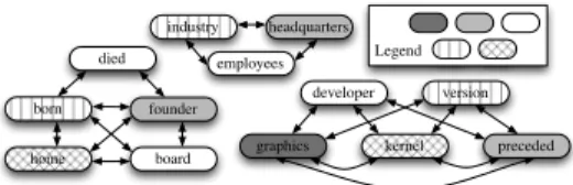
Figure 4: Graph Coloring Example

of datasetDwithmor fewer colors. All of our datasets (see Sec-tion 4 for details on them) except DBpedia could be colored to fit on a database row. When a coloring does not exist, as in DBpedia, this means there is no way to put all the predicates into the columns such that every entity can be placed on one row and each predicate for the entity be given exactly one column. In this case, we can color a subset of predicates (e.g., based on query workload and the most frequently occurring predicates), and compose a predicate mapping function based on this coloring and hash functions.

We define more formally what we mean by coloring for a subset. Specifically, we define a subsetP of the predicates in datasetD, and we writeD⊗P to be all triples inD that have a predicate fromP. If we chooseP such that the remaining data is colorable withm−1colors, then we define a mapping function

ˆ

cD_m⊗P≡

cD_m⊗₋P₁ p∈P m p /∈P

This coloring function can be composed with another function to handle the predicates not inP, for instanceˆcD⊗P

m ⊕hm. With this

predicate mapping composition, we were able to fit most of the data for a given entity on a single row, and reduce spills, while ensuring that the number of columns usage was minimized. Note that this same compositional approach can be used to handle dynamicity in data. If a new predicatepgets added after coloring, the second hash function is used to specify the column assignment forp.

Figure 4 shows how coloring works for the data in Figure 1(a). Predicatesdied, born, andfounderhave interference edges because they co-occur for entityCharles Flint. Similarly,founder,born,homeand

boardco-occur forLarry Pageand are hence connected. Notice fur-ther that the coloring algorithm will colorboardanddiedthe same color even though both are predicates for the same type of entity (e.g., Person) because they never co-occur together (in the data). Overall, for the 13 predicates, we only need 5 colors.

2.3

Graph Coloring in practice

We evaluated the effectiveness of coloring using four RDF datasets (see Section 4 for details). Our datasets were chosen so that they covered a wide range of skews and distributions [6]. So, for example, while the average out-degree in DBpedia is 14, in LUBM and SP2B it’s 6. The average in-degree in DBpedia is 5, in SP2B 2 and in LUBM 8. Beyond averages, out-degrees and in-degrees in DBpedia follow a power-law distribution [6] and therefore some subjects have significantly more predicates than others.

The results of graph coloring for all datasets are shown in Ta-ble 4. For the first three datasets, coloring covered 100% of the dataset, and reduced from 30% to as much as 85% the number of columns required in the DPH and RPH relations. So, while the LUBM dataset has 18 predicates, we only require 10 columns in the DPH and 3 in the RPH relations. In the one case where col-oring could not cover all the data, it could still handle 94% of the dataset in DPH with 75 columns, and 99% of the dataset in RPH with 51 columns, when we focused on the frequent predicates and the query workload. To put this in perspective, a one-to-one map-ping from predicates to columns would require 53,796 columns for DBpedia (instead of 75 and 51, respectively).

We now discuss spills and nulls. Ideally, we want to eliminate spills since they affect query evaluation. Indeed, by coloring in full

Dataset Triples Total DPH Percent. RPH Percent. Predicates Columns Covered Columns Covered SP2Bench 100M 78 54 100% 53 100% PRBench 60M 51 35 100% 9 100% LUBM 100M 18 10 100% 3 100% DBpedia 333M 53,976 75 94% 51 99%

Table 4: Graph Coloring Results

the first three datasets, we haveno spillsin the DPH and RPH rela-tions. So, storing 100M triples from LUBM inDB2RDFresults in 15,619,640 tuples in DPH (one per subject) and 11,612,725 tuples in RPH (one per object). Similarly, storing 100M triples of SP2B inDB2RDFresults in 17,823,525 in DPH and 47,504,066 tuples in RPH, without any spills. In DBpedia, storing 333M triples results in DPH and RPH relations with 23,967,748 and 78,697,637 tuples, respectively, with only 808,196 spills in the former (3.37% of the DPH) and 35,924 spills in the latter (0.04% of RPH). Of course, our coloring considered the full dataset before loading so it is inter-esting to investigate how successful coloring is (in terms of spills) if only a subset of the dataset is considered. Indeed, we tried color-ing only 10% of the dataset, uscolor-ing random samplcolor-ing of records. We used the resulted coloring from the sample to load the full dataset and counted any spills along the way. For LUBM, by only coloring 10% of the records, we were still able to load the whole dataset without any spills. For SP2B, loading the full dataset resulted in a negligible number of spills, namely, 139 spills (out of 17,823,525 entries) in DPH, and 666 (out of 47,504,066 entries) in RPH. More importantly, for DPpedia we only had 222,423 additional spills in DPH (a 0.9% increase in DPH) and 216,648 additional spills in RPH (a 0.3% increase). So clearly, our coloring algorithm per-forms equally well for bulk and for incremental settings.

In any dataset, each subject does not instantiate all predicates, and therefore even in the compressed (due to coloring) DPH and RPH relations not all subjects populate all columns. Indeed, our statistics show that for LUBM, in the DPH relation 64.67% of its predicate columns contain NULLs, while this number is 94.77% for the RPH relation. For DBpedia, the corresponding numbers are 93% and 97.6%. It is interesting to see how a high percentage of NULLs affects storage and querying. In terms of storage, exist-ing commercial (e.g.,IBM DB2) and open-source (e.g.,Postgres) database systems can accommodate large numbers of NULLs with small costs in storage, by usingvalue compression. Indeed, this claim is also verified by the following experiment. We created a 1M triples dataset in which each triple in the dataset had the same 5 predicates and loaded this dataset in ourDB2RDFschema using IBM DB2 as our relational back-end. The resulting DPH relation has 5 predicate columns and no NULL values (as expected) and its size on disk was approximately 10.1MB. We altered the DPH rela-tion and introduced (i) 5 addirela-tional null-populated predicate/value columns, (ii) 45 null-populated columns, or (iii) 95 null-populated columns. The storage requirements for these relations changed to 10.4MB, 10.65MB and 11.4MB respectively. So, increasing by 20-fold the size of the original relation with NULLs only required 10% of extra space.

We also evaluated queries across all these relations. The im-pact of NULLs is more noticeable here. We considered both fast queries with small result sets, and longer running queries with large result sets. The 20-fold increase in NULLs resulted in differences in evaluation times that ranged from as low as 10% to as much as a two-fold increase on the fastest queries. So, while the pres-ence of NULLs has small impact in storage, it can noticeably affect query performance, at least for very fast queries. This illustrates the value of our coloring techniques. By reducing both the number of columns with nulls, and the number of nulls in existing columns, we improve query evaluation and minimize space requirements.

Legend

Data Flow Builder

SPARQL Query Parse Tree Data Flow Graph Optimal Flow Tree Plan Builder Execution Tree SQL Builder Query Plan SQL Query Optimization Translation Statistics Access Methods

Figure 5: Query optimization and translation architeture

3.

QUERYING RDF

Relational systems have a long history of query optimization, so one might suppose that a naive translation fromSPARQLtoSQL would be sufficient, since the relational optimizer can optimize the SQLquery once the translation has occurred. However, as we show empirically here and in Section 4, huge performance gains can oc-cur whenSPARQLand theSPARQLtoSQLtranslation are indepen-dently optimized. In what follows, we first present a novel hy-bridSPARQL query optimization technique, which is generic and independent of our choice of representingRDFdata (in relational schema, or otherwise). In fact these techniques can be applied di-rectly to query optimization for nativeRDFstores. Then, we intro-duce query translation techniques tuned to our schema representa-tion. Figure 5 shows the steps of the optimization and translation process, as well as the key structures constructed at each step.

3.1

The SPARQL Optimizer

There are three inputs to our optimization:

1. The queryQ: TheSPARQLquery conforms to theSPARQL1.0 standard. Therefore, each queryQis composed of a set of hierar-chically nested graph patternsP, with each graph patternP ∈ P being, in its most simple form, a set of triple patterns.

2. The statisticsSover the underlyingRDFdataset: The types and precision with which statistics are defined is left to specific implementations. Examples of collected statistics include the total number of triples, average number of triples per subject, average number of triples per object, and the top-k URIs or literals in terms of number of triples they appear in, etc.

3. The access methodsM: Access methods provide alternative ways to evaluate a triple patterntfor some patternP ∈ P. The methods are system-specific, and dependent on existing indexes. For example, for a system likeDB2RDFwith only subject and ob-ject indexes (no predicate indexes), the methods would be access-by-subject(acs), byaccess-by-object(aco)or afull scan(sc).

Figure 6 shows a sample input where queryQretrieves the peo-ple that founded or are board members of companies in the software industry. For each such company, the query retrieves the products that were developed by it, its revenue, and optionally its number of employees. The statisticsScontain the top-k constants likeIBMor industrywith counts of their frequency in the base triples. Three different access methods are assumed in M, one that performs a data scan(sc), one that retrieves all the triples given a subject

(acs), and one that retrieves all the triples given an object(aco). The optimizer consists of two modules, namely, theData Flow BuilderDFB, and theQuery Plan BuilderQPB.

•Data Flow Builder (DFB): Query triple patterns typically share variables, and hence the evaluation of one is often dependent on that of another. For example, in Figure 6(a) triple patternt1shares variable?xwith both triples patternst2 andt3. InDFB, we use sideways information passing to construct an optimal flow tree, that considers cheaper patterns (in terms of estimated variable bindings) first before feeding these bindings to more expensive patterns. •Query Plan Builder (QPB):While theDFBconsiders informa-tion passing irrespectively of the query structure (i.e.,, the

nest-SELECT ?

WHERE{?xhome “Palo Alto” t1

{?xfounder ?y t2_UNION ?xmember ?y t3_} {?yindustry “Software” t4 ?zdeveloper ?y t5 ?yrevenue ?n t6_} OPTIONAL { ?yemployees ?mt7_{} }}

(a) Sample queryQ

value count

IBM 7

industry 6

Google 5

Software 2

Avg triples per subject 5 Avg triples per object 1 Total triples 26

(b) top-k stats inS

M= {sc,acs,aco}

(c) Access methodsM

Figure 6: Sample input for query optimization/translation

ANDT t1 t2 t3 t4 t5 t6 t7 ANDN OR OPTIONAL

Figure 7: Query parse tree

(t5, acs) (t4, acs) (t6, aco) (t2, acs) (t3, acs) (t1, aco) (t7, aco) (t4, aco) (t5, aco) (t6, acs) (t7, acs) (t2, aco) (t3, aco) (t1, acs)

Figure 8: Data flow graph ing of patterns and pattern operators), the QPBmodule incorpo-rates this structure to build an execution tree (a storage-independent query plan). Our query translation (Section 3.2) uses this execution tree to produce a storage specific query plan.

3.1.1

The Data Flow Builder

TheDFBstarts by building a parse tree for the input query. The tree for the query in Figure 6(a) is shown in Figure 7. Then it uses sideways information passing to compute the data flow graph which represents the dependences amongst the executions of each triple pattern. A node in this graph is a pair of a triple pattern and an access method; an edge denotes one triple producing a shared vari-able that another triple requires. Using this graph,DFBcomputes the optimal flow tree (the blue nodes in Figure 7) which determines an optimal way (in terms of minimizing costs) to traverse all the triple patterns in the query. In what follows, we describe in detail how all these computations are performed.

Computing cost.

Definition 3.1(Triple Method Cost). Given a triplet, an access methodmand statisticsS, functionTMC(t, m,S) :→c, c∈R≤0 assigns a costcto evaluatingtusingmwrt statisticsS.

The cost estimation clearly depends on the statistics S. In our example, TMC(t4, aco,S) = 2 because the exact lookup cost using the object Software is known. For a scan method, TMC(t4, sc,S) = 26,i.e.,the total number of triples in the dataset. Finally,TMC(t4, acs,S) = 5,i.e.,the average number of triples per subject, assuming subject is bound by a prior triple access.

Building the Data Flow Graph.

The data flow graph models how using the current set of bind-ings for variables can be used to access other triples. In model-ing this flow, we need to respect the semantics ofAND,ORand

OPTIONALpatterns. We first introduce a set of helper functions that are used to define the graph. We use↑to refer to parents in the query tree structure: for a triple or a pattern, it is the immediately enclosing pattern. We use∗to denote transitive closure.

Definition 3.2(Produced Variables). P(t, m) :→ Vprodmaps a

triple and an access method pair to a set of variables that are bound after the lookup, wheretis a triple,mis an access method, and Vprodis the set of variables.

In our example, for the pair(t4, aco),P(t4, aco) :→y, because the lookup usesSoftwareas an object, and the only variable that gets bound as a result of the lookup isy.

Definition 3.3(Required Variables). R(t, m) :→ Vreq maps a

triple and an access method pair to a set of variables that are re-quired to be bound for the lookup, wheretis a triple, mis an access method, andVreqis the set of variables.

Back to the example,R(t5, aco) :→y. That is, if one uses the acoaccess method to evaluatet5, then variableymust be bound by some prior triple lookup.

Definition 3.4(Least Common Ancestor). LCA(p, p0)is the first common ancestor of patternspandp0. More formally, it is defined as follows:

LCA(p, p0) =x ⇐⇒

x∈ ↑∗_{(p)∧x∈ ↑}∗_(p0_)∧

@y.y∈ ↑∗(p)∧y∈ ↑∗(p0)∧x∈ ↑∗(y) As an example, in the Figure 7, the least common ancestor of ANDNandORisANDT.

Definition 3.5(Ancestors ToLCA). ↑↑(p, p0)refers to the set of ↑∗built from traversing frompto theLCA(p, p0):

↑↑(p, p0)≡_x

x∈ ↑

∗_(p)

∧ ¬x∈ ↑∗(LCA(p, p0))

For instance, for the query shown in Figure 7, ↑↑

(t1,LCA(t1, t2)) ={ANDT,OR}

Definition 3.6(ORConnected Patterns). ∪denotes that two triples are related in anORpattern, i.e. their least common ancestor is an ORpattern:∪(t, t0)≡LCA(t, t0)isOR.

In the example,t2andt3are∪.

Definition 3.7(OPTIONALConnected Pattern). OPTIONAL Con-nected Patterns∩ˆdenotes if one triple is optional with respect to another, i.e. there is an OPTIONAL pattern guardingt0 with re-spect tot:

ˆ

∩(t, t0_{)≡ ∃p:p∈ ↑↑(t}0_{, t)∧pisOPTIONAL}

In the example, t6 and t7 are∩, becauseˆ t7 is guarded by an OPTIONALin relation tot6.

Definition 3.8 (Data Flow Graph). The Data Flow Graph is a graph ofG =< V, E >, whereV = (T × M)∪root, where

root is a special node we add to the graph. A directed edge

(t, m)→(t0, m0)exists inV when the following conditions hold:

P(t, m)⊃ R(t0, m0)∧ ¬ ∪(t, t0)∨∩ˆ(t0, t)

In addition, a directed edge fromrootexists to a node(t, m)if R(t, m) =∅.

In the example , a directed edgeroot →(t4, aco)exists in the data flow graph (in Figure 8 we show the whole graph but for simplicity in the figure we omit the rootnode), because t4 can be accessed by an object with a constant, and it has no required variables. Further,(t4, aco) → (t2, aco)is part of the data flow graph, because(t2, aco)has a required variableythat is produced by(t4, aco). In turn,(t2, aco)has an edge to(t1, acs), because

(t1, acs)has a required variablexwhich is produced by(t2, aco).

TheData Flow GraphGis weighted, and the weights for each edge between two nodes is determined by a function:

W((t, m),(t0, m0)),S) :→w

The w is derived from the costs of the two nodes, i.e., TMC(t, m,S), andTMC(t0, m0,S). A simple implementation of this function, for example could apply the cost of the target node to the edge. In the example, for instance,wfor the edgeroot →

(t4, aco)is 2, whereas the edgeroot→(t4, asc)is 5.

Computing The Optimal Flow Tree.

Given a weighted data flow graphG, we now study the problem of computing the optimal (in terms of minimizing the cost) order for accessingallthe triples in queryQ.

Theorem 3.1. Given a data flow graphGfor a queryQ, finding the minimal weighted tree that covers all the triples inQis NP-hard.

The proof is by reduction from the TSP problem and is omitted here due to lack of space. In spite of this negative result, one might think that the input queryQis unlikely to contain a large number of triples, so an exhaustive search is indeed possible. However, even in our limited benchmarks, we found this solution to be impractical (e.g., one of our queries in the tool integration benchmark had 500 triples, spread across 100ORpatterns). We therefore introduce a greedy algorithm to solve the problem: LetT denote the execu-tion treewe are trying to compute. Letτ refer to the set of triples corresponding to nodes already in the tree:

τ≡ {ti|∃mi (ti, mi)∈ T }

We want to add a node that adds a new triple to the tree while adding the cheapest possible edge; formally, we want to choose a node(t0, m0)such that

(t0_{, m}0_{)∈V ∧ # node to add} t0∈/τ∧ # node adds new triple

∃(t, m) :             

(t, m)∈ T ∧ # node currently in tree

(t, m)→(t0, m0)∧ # valid edge to new node # no similar pair of nodes such that...

@(t00, m00),(t000, m000) :      (t00, m00)∈ T ∧ t000∈/τ∧ (t00, m00)→(t000, m000)∧ # ...adding(t000, m000)is cheaper W((t00, m00),(t000, m000))<W((t, m),(t0, m0))                  

On the first iteration,T0=root, andτ0=∅.Ti+1is computed by applying the step defined above, and the triple of the chosen node is added toτi+1. In our example,root → (t4, aco)is the cheapest edge, soT1 = (t4, aco), andτ0 = t4. We then add

(t2, aco)toT2, and so on. We stop when we get toTn, wheren

is the number of triples inQ. Figure 8 shows the computed tree (marked blue nodes) while Figure 9 shows the algorithm, where functiontriple(j)returns the triple associated with a node inG.

3.1.2

The Query Plan Builder

Both the data flow graph and the optimal flow tree largely ignore the query structure (the organization of triples into patterns) and the operators between the (triple) patterns. Yet, they provide useful in-formation as to how to construct an actual plan for the input query, the focus of this section and output of theQPBmodule.

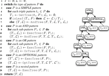
In more detail, Figure 10 shows the main algorithmExecTreeof the module. The algorithm is recursive and takes as input the opti-mal flow treeFcomputed byDFB, and (the parse tree of) a pattern P, which initially is the main pattern that includes the whole query

Input: The weighted data flow graphG

Output: An optimal flow treeT

1 τ← ∅;

2 T ←root;

3 E←SortEdgesByCost(G);

4 while|T |<|Q|do

5 foreach edgeeij∈Edo

6 ifi∈ T ∧j /∈ T ∧triple(j)6∈τthen

7 T ← T ∪j;

8 τ←τ∪triple(j);

9 T←eij;

Figure 9: The algorithm for computing the optimal flow tree

Input: The optimal flow treeFof queryQ, a patternPinQ

Output: An execution treeTforP, a setLof execution sub-trees

1 T← ∅;L ← ∅;

2 switchthe type of patternPdo

3 casePis a SIMPLE pattern 4 foreach triple patternti∈Pdo

5 Ti←GetTree(ti, F);Li← ∅;

6 ifisLeaf(Ti,F)thenL ← L ∪Ti;

7 else (T ,L)←AndTree(F,T,L,Ti,Li);

8 casePis an AND pattern 9 foreach sub-patternPi∈Pdo

10 (Ti,Li)←ExecTree(F,Pi);

11 (T ,L)←AndTree(F,T,L,Ti,Li);

12 casePis an OR pattern 13 foreach sub-patternPi∈Pdo

14 (Ti,Li)←ExecTree(F,Pi);

15 (T ,L)←OrTree(F,T,LTi,Li);

16 casePis an OPTIONAL pattern

17 (T0,L0)←ExecTree(F,P);

18 (T ,L)←OptTree(F,T,LT0,L0);

19 casePis a nested pattern

20 (T ,L)←ExecTree(F,P); 21 return(T ,L) AND1 OR1 AND2 AND3 AND4 OPTIONAL1 AND5 (t4, aco) (t2, aco) (t3, aco) (t1, acs) (t5, aco) (t6, acs) (t7, acs)

Figure 10: TheExecTreeAlgorithm and resulting execution tree Q. So in our running example, for the query in Figure 6(a), the algorithm takes as input the parse tree in Figure 7 and the optimal flow tree in Figure 8. The algorithm returns a schema-independent planT, called theexecution treefor the input query patternP. The set of returned execution sub-treesLis guaranteed to be empty when the recursion terminates, but contains important information that the algorithm passes from one level of recursion to the previous one(s), while the algorithm runs (more on this later).

There are four main types of patterns inSPARQL, namely, SIM-PLE,AND, UNION(a.k.aOR), andOPTIONAL patterns, and the algorithm handles each one independently, as we illustrate through our running example. Initially, both the execution treeT and the setLare empty (line 1). Since the top-level node in Figure 7 is an ANDnode, the algorithm considers each sub-pattern of the top-level node and calls itself recursively (lines 8-10) with each of the sub-patterns as argument. The first sub-pattern recursively considered is aSIMPLEone consisting of the single triple patternt1. By consult-ing the flow treeF, the algorithm determines the optimal execution tree fort1which consists of just the node(t1, acs)(line 5). By fur-ther consulting the flow (line 6) the algorithm determines that node

(t1, acs)is a leaf node in the optimal flow and therefore it’s eval-uation depends on the evaleval-uation of other flow nodes. Therefore, the algorithm adds tree(t1, acs)to the locallate fusingsetLof execution trees. SetLcontains execution sub-trees that should not be merged yet with the execution treeT but should be considered later in the process. Intuitively, late fusing plays two main roles: (a) it uses the flow as a guide to identify the proper point in time to fuse the execution treeT with execution sub-trees that are already computed by the recursion; and (b) it aims to optimize query eval-uation by minimizing the size of intermediate results computed by the execution tree, and therefore it only fuses sub-trees at the lat-est possible place, when either the corresponding sub-tree variables are needed by the later stages of the evaluation, or when the

oper-ators and structure of the query enforce the fuse. The first recur-sion terminates by returning(T1,L1) = (∅,{L1 = (t1, acs)}). The second sub-pattern in Figure 7 is anORand is therefore han-dled in lines 12-15. The resulting execution sub-tree contains three nodes, anORnode as root (from line 15) and nodes(t2, aco)and

(t3, aco) as leaves (recursion in line 14). This sub-tree is also added to local set Land the second recursion terminates by re-turning(T2,L2) = (∅,{L2 ={OR,(t2, aco),(t3, aco)}}). Fi-nally, the last sub-pattern in Figure 7 is an AND pattern again, which causes further recursive calls in lines 8-11. In the recur-sive call that processes triplet4(lines 5-7), the execution tree node

(t4, aco) is the root node in the flow and therefore it is merged to the main execution treeT. SinceT is empty, it becomes the root of the treeT. The three sub-trees that include nodes(t5, aco),

(t6, acs), andOP T ={(OPTIONAL),(t7, aco)}are all becoming part of setL. Therefore, the third recursion terminates by return-ing(T3,L3) = ((t4, aco),{L3={(t5, aco)}, L4={(t6, acs)}, L5={(OPTIONAL),(t7, aco)}}. Notice that after each recursion ends (line 10), the algorithm considers (line 11) the returned ex-ecutionTi and late-fuseLi trees and uses functionAndTreeto

build a new local executionT and set Lof late-fusing trees (by also consulting the flow and following the late-fusing guidelines on postponing tree fusion unless it is necessary for the algorithm to progress). So, after the end of the first recursion and the first call to functionAndTree,(T ,L) = (T1,L1),i.e.,, the trees returned from the first recursion. After the end of the second recursion, and the second call toAndTree,(T ,L) = (∅,L1∪ L2). Finally, after the end of the third recursion,(T ,L) = ((t4, aco),L1∪ L2∪ L3). The last call toAndTreebuilds the tree to the right of Figure 10 in the following manner. Starting from node(t4, aco), it consults the flow and picks from the set Lthe sub-treeL2 and connects this to node(t4, aco)by adding a newANDnode as the root of the tree. Sub-treesL3,L4andL5can be added at this stage toT but they are not considered as they violate the principles of late-fusing (their respective variables are not used by any other triple, as is also obvious by the optimal flow). On the other hand, there is still a de-pendency between the latest treeTandL1since the selectivity of t1can be used to reduce the intermediate size of the query results (especially the bindings to variable?y). Therefore, a newANDis introduced and the existingTis extended withL1. The process it-erates in this fashion until the whole tree in Figure 10 is generated. Note that by using the optimal flow tree as a guide, we are able toweavethe evaluation of different patterns, while our structured-based processing guarantees that the associativity of operations in the query is respected. So, our optimizer can generate plans like the one in Figure 10 where only a portion of a pattern is initially evaluated (e.g.,node(t4, aco)) while the evaluation of other con-structs in the pattern (e.g.,node(t5, aco)) can be postponed until it no longer can be avoided. At the same time, this de-coupling from query structure allow us to safely push the evaluation of patterns early in the plan (e.g.,node(t1, acs)) when doing so improves se-lectivity and reduces the size of intermediate results.

3.2

The SPARQL to SQL Translator

The translator takes as input the execution tree generated from theQPBmodule and performs two operations: first, it transforms the execution tree into an equivalent query plan that exploits the entity-oriented storage ofDB2RDF; second, it uses the query plan to create theSQLquery which is executed by the database.

3.2.1

Building the Query Plan

The execution tree provides an access method and an execution order for each triple but assumes that each triple node is evaluated

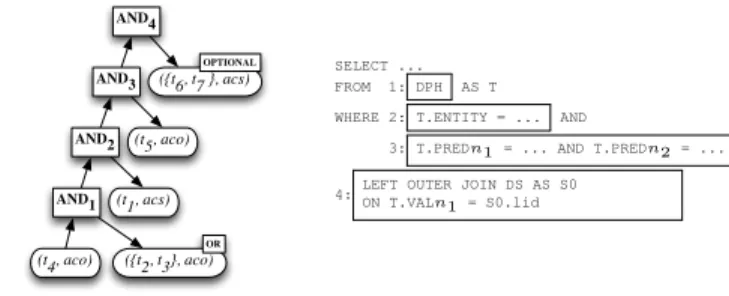
AND1 AND2 AND3 AND4 (t4, aco) ({t2, t3}, aco) (t1, acs) (t5, aco) ({t6, t7 }, acs) OR OPTIONAL

Figure 11: The query plan tree

SELECT ... FROM 1: DPH AS T WHERE 2: T.ENTITY = ... AND

3: T.PREDn1 = ... AND T.PREDn2= ...

4:LEFT OUTER JOIN DS AS S0 ON T.VALn1 = S0.lid

Figure 12: SQL code template independently of the other nodes. However, one of the advantages of the entity-oriented storage is that a single access to, say, the DPH relation might retrieve a row that can be used to evaluate multiple triple patterns (star-queries). To this end, starting from the exe-cution tree the translator builds a query plan where triples with the same subject (or the same object) aremergedin the same plan node. A merged plan node indicates to theSQLbuilder that the containing triples form a star-query and must be executed with a singleSQL select. Merging of nodes is always advantageous with one excep-tion: when the star query involves entities with spills. The pres-ence of such entities would require self-joins of the DPH (RPH) relations in the resultingSQLstatement. Self-joins are expensive and therefore we use the following strategy to avoid them: When weknowthat star-queries involve entities with spills, we choose to cascadethe evaluation of the star-query by issuing multipleSQL statements, each evaluating a subset of the star-query while at the same time filtering entities from the subsets of the star-query that have been previously evaluated. The multipleSQLstatements are such that noSQLstatement accesses predicates stored into different spill rows. Of course, the question remains on how we determine whether spills affect a star query. In our system this is straightfor-ward. With only a tiny fraction of predicates involved in spills (due to coloring – see Section 2.3), our optimizer consults an in-memory structure of predicates involved in spills to determine during merg-ing whether any of the star-query predicates participate in spills.

During the merging process we need to respect both the struc-turalandsemanticconstraints. The structural constraints are im-posed by the entity-oriented representation of data. To satisfy the structural constraints, candidate nodes for merging need to refer to the same entity, have the same access method and do not involve spills. As an example, in Figure 8 nodest2andt3refer to the same entity (due to variable?x) and the same access methodaco, as do nodest6andt7, due to the variable?yand the methodacs.

Semantic constraints for merging are imposed by the control structure of theSPARQLquery (i.e.,theAND,UNION,OPTIONAL patterns). This restricts the merging of triples to constructs for which we can provide the equivalentSQLstatements to access the relational tables. Triples in conjunctive and disjunctive patterns can be safely merged because the equivalentSQLsemantics are well un-derstood. Therefore, with a single access we can check whether the row includes the non-optional predicates in the conjunction. Sim-ilarly, it is possible to check the existence of any of the predicates mentioned in the disjunction. More formally, to satisfy the seman-tic constraints ofSPARQL, candidate nodes for merging need to be ANDMergeable,ORMergeableorOPTMergeable.

Definition 3.9 (AND Mergeable Nodes). Two nodes are ANDMergeableiff their least common ancestor and all intermediate ancestors areANDnodes:

ANDMergeable(t, t0) ⇐⇒

∀x:x∈(↑↑(t,LCA(t, t0))∪ ↑↑(t0,LCA(t, t0))) =⇒ xisAND Definition 3.10 (OR Mergeable Nodes). Two nodes are

ORMergeableiff their least common ancestor and all intermediate ancestors areORnodes:

ORMergeable(t, t0) ⇐⇒

∀x:x∈(↑↑(t,LCA(t, t0))∪ ↑↑(t0,LCA(t, t0))) =⇒ xisOR Going back to the execution tree in Figure 10, notice that ORMergeable(t2, t3) is true, butORMergeable(t2, t5) is false. Definition 3.11 (OPTIONAL Mergeable Nodes). Two nodes are OPTMergeableiff their least common ancestor and all intermedi-ate ancestors areANDnodes, except the parent of the higher order triple in the execution plan which isOPTIONAL:

OPTMergeable(t, t0) ⇐⇒

∀x:x∈(↑↑(t,LCA(t, t0))∪ ↑↑(t0,LCA(t, t0))) =⇒ xisAND ∨ {xisOPTIONAL ∧xis parent oft0} As an example, in Figure 10OPTMergeable(t6, t7) is true. Given the input execution tree, we identify pairs of nodes that satisfyboththe structural and semantic constraints introduced, and we merge them. Due to lack of space, we omit here the full details of the node merging algorithm and illustrate the output of the al-gorithm for our running example. So, given as input the execution tree in Figure 10, the resulting query plan tree is shown in Fig-ure 11. Notice that in the resulting query plan there are two node merges, one due to the application of theORMergeabledefinition, and one by the application of theOPTMergeabledefinition. Note that each merged node is annotated with the corresponding seman-tics under which the merge was applied. As a counter-example, consider node(t5, aco)which is compatible structurally with the new node({t2, t3}, aco)since they both refer to the same entity through variable?y, and have the same access methodaco. How-ever, these two nodes are not merged since they violate the semantic constraints (i.e.,they do not satisfy the definitions above since their merge would mix a conjunctive with a disjunctive pattern). Even for our simple running example, the two identified node merges re-sult in significant savings in terms of query evaluation. Intuitively, one can think of these two merges as eliminating two extra join op-erations during the translation of the query plan to an actualSQL query over theDB2RDFschema, the focus of our next section.

3.2.2

The

Generation

SQLgeneration is the final step of query translation. The query plan tree plays an important role in this process, and each node in the query plan tree, be it a triple, merge or control node, contains the necessary information to guide theSQLgeneration. For the gen-eration, theSQLbuilder performs a post order traversal of the query plan tree and produces the equivalentSQLquery for each node. The whole process is assisted by the use ofSQLcode templates.

In more detail, the base case ofSQLtranslation considers a node that corresponds to a single triple or a merge. Figure 12 shows the template used to generateSQLcode for such a node. The code in box 1 sets the target of the query to the DPH or RPH tables, ac-cording to the access method in the triple node. The code in box 2 restricts the entities being queried. As an example, when the subject is a constant and the access method isacs, theentryis connected to the constant subject values. When the subject is variable and the method isacs, thenentryis connected with a previously-bound variable from a priorSELECTsub-query. The same reasoning ap-plies for theentrycomponent for an object when the access method isaco. Box 3 illustrates how one or more predicates are selected. That is, when the plan node corresponds to a merge, multiplepredi

components are connected through conjunctive or disjunctiveSQL operators. Finally, box 4 shows how we do outer join with the sec-ondary table for multi-valued predicates.

WITH QT4RPH AS

SELECTT.val₁ASval₁FROMRPHASTWHERET.entry=’Software’ANDT.pred₁=’industry’,

QT4DS AS

SELECT COALESCE(S.elm, T.val₁)ASy

FROM QT4RPH ASTLEFT OUTER JOINDSASSONT.val₁=S.l_id QT₂₃RPH AS

SELECT QT₄DS.y,

CASET.pred_m=’founder’THENvalmELSEnullEND ASvalm,

CASET.pred₀=’member’THENval₀ELSEnullEND ASval₀

FROM RPHAST,QT₄DS

WHERET.entry=QT₄DS.yAND(T.pred_m=’founder’ORT.pred₀=’member’),

QT₂₃AS

SELECTLT.val₀ASx, T.yFROM QT₂₃RPHas T,TABLE(T.valm, T.val₀) as LT(val₀)

WHERELT.val₀IS NOT NULL QT₁DPH AS

SELECTT.entryASx,QT₂₃.yFROMDPHAST,QT₂₃ WHERET.entry=QT23.xANDT.pred_k=’home’ANDT.val₁=’Palo Alto’,

QT5RPH AS

SELECTT.entryASy,QT1DPH.xFROMRPHAST,QT1DPH WHERET.entry=QT1DPH.yANDT.pred₁=’developer’,

QT67DPH AS

SELECTT.entryASy,QT5RPH.x,CASET.pred_k=’employees’THENval_kELSEnullENDas z

FROM DPHAST,QT5RPH WHERET.entry=QT5RPH.yANDT.pred_m=’revenue’

SELECTx, y, zFROM QT67DPH

Figure 13: GeneratedSQLforSPARQLQuery in Figure 6 The operator nodes in the query plan are used to guide the con-nection of instantiated templates like the one in Figure 12. We have already seen howAND nodes are implemented through the vari-able binding across triples as in box 2. ForORnodes we use the SQLUNIONoperator to connect its components’ previously defined SELECTstatements. ForOPTIONALwe use LEFT OUTER JOIN between theSQLtemplate for the main pattern and theSQL tem-plate for theOPTIONALpattern. Figure 13 shows the finalSQLfor our running example where theSQLtemplates described above are instantiated according to the query plan tree in Figure 11.

In Figure 13, several Common Table Expressions (CTEs) are used for each plan node.t4is evaluated first and accesses RPH us-ing theSoftwareconstant. Sinceindustryis a multivalued predicate, the RS table is also accessed. The remaining predicates in this example are single valued and the access to the secondary table is avoided. TheORMergeablenodet23is evaluated next using the RPH table where the object is bound to the values ofyproduced by the first triple. TheWHEREclause enforces the semantic that at least one of the predicates is present. The CTE projects the values corre-sponding to the present predicates and null values for those that are missing. The next CTE just flips these values, creating a new result record for each present predicate. The plan continues with triplet5 and is completed with node theOPTMergeablenodet67. Here no constraint is imposed for the optional predicate making its presence optional on the record. In case the predicate is present, the corre-sponding value is projected, otherwise null. In this example, each predicate is assigned to a single column. When predicates are as-signed to multiple columns, the position of the value is determined with CASE statements as seen in theSQLsample.

3.3

Advantages of the SPARQL Optimizer

To examine the effectiveness of our query optimization, we conducted experiments using both our 1M triple microbenchmark of Section 2.1 (which offers more control) and queries from the datasets used in our main experimental section (Section 4). As an example, for our microbenchmark we considered two constant val-uesO1andO2with relative frequency in the data of .75 and .01, re-spectively. Then, we issued the simple query shown in Figure 14(a) that allowed data flows in either direction; i.e., evaluation could start ont1with anacousingO1, then use the bindings for?sto ac-cesst2with anacs, or start instead ont2with anacousingO2and use bindings for?sto accesst1. The latter case is of course better. Figure 14(b) shows the SQL generated by ourSPARQLoptimizer while Figure 14(c) shows an equivalentSQLquery corresponding to the only alternative but sub-optimal flow. The former query took 13 ms to evaluate, whereas the latter took 5X longer, that is 65 ms, suggesting that our optimization is in fact effective even in this

SELECT ?sWHERE{?sSV₁O₁ t1.?sSV₂O₂t2} (a) SPARQL Query

SELECTT.ENTRY, D.ENTRYFROMRS AS R, DPH AS D

WHERE R.ENTRY=’O₂’ANDR.PROP=’SV₂’ANDD.ENTRY=T.ENTRYANDD.VAL0=’O₁’ANDD.PROP0=’SV₁’ (b) Optimized SQL

SELECTT.ENTRY, D.ENTRYFROMRS AS R, DPH AS D

WHERER.ENTRY=’O₁’ AND R.PROP=’SV₁’ANDD.ENTRY=T.ENTRYANDD.VAL0=’O₂’ANDD.PROP0=’SV₂’ (c) Alternative SQL

Figure 14: Query Translation

simple query. Using real and benchmark queries from datasets re-sulted in even more striking differences in evaluation times. For ex-ample, when optimized by ourSPARQLoptimizer query,PQ1from PRBench (Section 4) was evaluated in 4ms, while the translated SQLcorresponding to a sub-optimal flow required 22.66 seconds!

4.

EXPERIMENTS

We compared the performance ofDB2RDF, using IBM DB2 as our relational back-end, to that of Virtuoso 6.1.5 OpenSource Edi-tion, Apache Jena 2.7.3 (TDB), OpenRDF Sesame 2.6.8, and RDF-3X 0.3.5. DB2RDF, Virtuoso and RDF-3X were run in a client server mode on the same machine and all other systems were run in process mode. For both Jena and Virtuoso, we enabled all recom-mended optimizations. Jena had the BGP optimizer enabled. For Virtuoso we built all recommended indexes. ForDB2RDF, we only added indexes on the entry columns of the DPH and RPH relations (no indexes on theprediandvalicolumns).

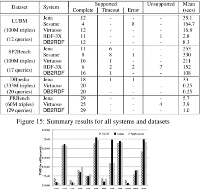
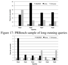
We conducted experiments with 4 different benchmarks: LUBM [7], SP2Bench [15], DBpedia [12], and a private benchmark PRBench that was offered to us by an external partner organization. For the LUBM and SP2Bench benchmarks, we scaled them up to 100 million triples each and used their associated published query workloads. The DBpedia 3.7 benchmark [5] has 333 million triples. The private benchmark included data from a tool integration appli-cation, and it contained 60 million triples about various software ar-tifacts generated by different tools (e.g., bug reports, requirements, etc). For all systems, we evaluated queries in a warm cache sce-nario. For each dataset, benchmark queries were randomly mixed to create a run, and each run was issued 8 times to the 5 stores. We discarded the first run and reported the average result for each query over 7 consecutive runs. For each query, we measured its running time excluding the time taken to stream back the results to the API, in order to minimize variations caused by the various APIs avail-able. As shown in Figure 15, the evaluated queries were classified into four categories. Queries that failed to parseSPARQLcorrectly, we reported asunsupported. The remainder supported queries were further classified as eithercomplete,timeout, orerror. We counted the results from each system and when a system provided the cor-rect number of answers we classified the query as completed. If the system returned the wrong number of results, we classified this as an error. Finally, we used a timeout of 10 minutes to trap queries that do not terminate within a reasonable amount of time. In the figure, we also report the average time taken (in seconds) to eval-uate complete and timeout queries. For queries that timeout, their running time was set to 10 minutes. For obvious reasons, we do not count the time of queries that return the wrong number of results.

This is the most comprehensive evaluation of RDF systems. Un-like previous works, this is the first study that evaluates 5 systems using a total of78 queries, over a total of600 million triples. Our experiments were conducted on 5 identical virtual machines (one per system), each equivalent to a 4-core, 2.6GHz Intel Xeon sys-tem with 32GB of memory running 64-bit Linux. Each syssys-tem was