Go Beyond VFP's SQL with SQL
Server
Tamar E. Granor Tomorrow's Solutions, LLC Voice: 215-635-1958 Email: [email protected]The subset of SQL in Visual FoxPro is useful for many tasks. But there's much more to SQL than what VFP supports. Those additions make it easy to do a number of tasks that are difficult in VFP.
In this session, we'll solve some common problems, using SQL elements that are supported by SQL Server, but not by VFP. Among the problems we'll explore are combining a set of values contained in multiple records into a delimited list in a single record, working with
hierarchical data like corporate organization charts, finding the top N records for each group in a result, and including summary records in grouped data.
Introduction
When FoxPro 2.0 was released nearly 25 years ago, it included some SQL commands. I fell in love as soon as I started playing with them. Over the years, Visual FoxPro’s SQL subset has grown, but there are still some tasks that are hard or impossible to do with SQL alone in VFP, but a lot easier in other SQL dialects. In this session, I’ll take a look at some of these tasks, showing you how VFP requires a blend of SQL and Xbase code, but SQL Server allows them to be done with SQL code only.
You’re unlikely to be choosing whether to store your data in VFP or in SQL Server based on which one makes these tasks easier. However, when you switch from working with VFP databases to working with SQL Server databases, it’s easy to just keep doing things the way you have been. The goal of this session is to show you how you can code better in SQL Server by learning some new approaches.
The VFP examples in this session use the example Northwind database. Most of the SQL examples in this session use the example AdventureWorks 2008 database, which you can download from http://tinyurl.com/cp2fv8w. One group of examples uses the
AdventureWorks 2005 database, because the 2008 version no longer includes the structure being discussed; you can download AdventureWorks 2005 from
http://tinyurl.com/y943xr9.
Consolidate data from a field into a list
One of the most common questions I see in online VFP forums is how to group data, consolidating the data from a particular field. If the consolidation you want is counting, summing, or averaging, the task is simple; just use GROUP BY with the corresponding aggregate function.
But if you want to create a comma-separated list of all the values or something like that, there’s no SQL-only way to do it in VFP. SQL Server, however, provides not one, but two, ways.
The VFP way
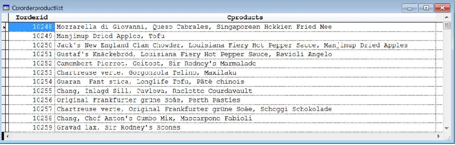
Using the Northwind database that comes with VFP, suppose you want (say, for reporting purposes) to have a list of orders, with a comma-separated list of the products included in each order, something like what you see in Figure 1.
Figure 1. This cursor includes each order from the Northwind database with a comma-separated list of the products ordered.
VFP’s SQL commands offer no way to combine the products like that. Instead, you have to run a query to collect the raw data and then use a loop to combine the products for each order. Listing 1 shows the code used to produce the cursor for the figure. (Like all the VFP examples in this paper, this one assumes you’ve already opened the Northwind database.)
Listing 1. To consolidate data into a comma-separated list in VFP requires a combination of SQL and Xbase code.
SELECT DISTINCT Orders.OrderID, Products.ProductName ; FROM Orders ;
JOIN OrderDetails ;
ON Orders.OrderID = OrderDetails.OrderID ; JOIN Products ;
ON OrderDetails.ProductID = Products.ProductID ; ORDER BY Orders.OrderID, ProductName ;
INTO CURSOR csrOrderProducts
LOCAL cProducts, cCurOrderID
CREATE CURSOR csrOrderProductList (iOrderID I, cProducts C(150))
SELECT csrOrderProducts
cCurOrderID = csrOrderProducts.OrderID cProducts = ''
SCAN
IF csrOrderProducts.OrderID <> m.cCurOrderID * Finished this order
INSERT INTO csrOrderProductList ;
VALUES (m.cCurOrderID, SUBSTR(m.cProducts, 3)) cProducts = ''
cCurOrderID = csrOrderProducts.OrderID ENDIF
cProducts = m.cProducts + ', ' + ALLTRIM(csrOrderProducts.ProductName) ENDSCAN
The query uses DISTINCT because we only want to include each product in the list once for each order. It also sorts the results by OrderID, which is necessary for the SCAN loop, and then by name within the order, so the result has the products in alphabetical order. The SCAN loop builds up the list of products for a single order and then when we reach a new order, adds a record to the result cursor and clears the cProducts variable, so we can start over for the new order.
The code in Listing 1 is included in the materials for this session as VFPProductsByOrder.PRG
The SQL way
SQL Server offers two ways to solve this problem. Each approach teaches something about elements of SQL Server that don’t exist in VFP’s SQL, so we’ll look at both.
Using the AdventureWorks 2008 database, to get an example analogous to the VFP
example, we can join the PurchaseOrderDetail table to the Product table to get a list of the products included in each purchase order, as in Listing 2.
Listing 2. This query, based on the AdventureWorks 2008 database, produces a list of products for each purchase order.
SELECT PurchaseOrderID, Name FROM Production.Product
Inner Join Purchasing.PurchaseOrderDetail
On Production.Product.ProductID = PurchaseOrderDetail.ProductID ORDER BY PurchaseOrderID
We’ll use this query as a basis for getting one record per purchase order with the list of products comma-separated.
FOR XML
The first approach uses the FOR XML clause. In general, this clause allows you to convert SQL results to XML. There are four variations of FOR XML; three of them produce XML results and vary only in how much control you have over the format of the result. For example, if you add the clause FOR XML AUTO at the end of the query in Listing 2, you get results like those in Listing 3.
Listing 3. Adding FOR XML AUTO to the query in Listing 2 produces this XML. (Only a few records are shown.)
<A PurchaseOrderID="1">
<Production.Product Name="Adjustable Race" /> </A>
<A PurchaseOrderID="2">
<Production.Product Name="Thin-Jam Hex Nut 9" /> <Production.Product Name="Thin-Jam Hex Nut 10" /> </A>
<Production.Product Name="Seat Post" /> </A>
<A PurchaseOrderID="4">
<Production.Product Name="Headset Ball Bearings" /> </A>
Using FOR XML RAW, instead, produces one element of type <row> for each record, with each field included as an attribute. Listing 4 shows the first few records of the result.
Listing 4. FOR XML RAW produces simpler XML.
<row PurchaseOrderID="1" Name="Adjustable Race" /> <row PurchaseOrderID="2" Name="Thin-Jam Hex Nut 9" /> <row PurchaseOrderID="2" Name="Thin-Jam Hex Nut 10" /> <row PurchaseOrderID="3" Name="Seat Post" />
A third version, FOR XML EXPLICIT, gives you tremendous control over the format of the output, at the cost of writing a more complex query. The details are beyond the scope of this session, and the documentation indicates that you can do the same things using FOR XML PATH much more easily. However, if you’re interested, see
http://technet.microsoft.com/en-us/library/ms189068.aspx.
The fourth version of FOR XML, using the PATH keyword, provides what we need to consolidate the product data into a single record. FOR XML PATH treats columns as XPath expressions. XPath, which stands for XML Path language, lets you select items in an XML document. Again, the full details are beyond the scope of this article.
What you need to know to solve the problem of creating a comma-separated list is that if you specify FOR XML PATH(''), the expression you specify in the query is consolidated into a single list, rather than one record per value. For example, the query in Listing 5 produces the results shown in Listing 6.
Listing 5. Use FOR XML PATH('') to combine data into a single string.
SELECT ', ' + Name FROM Production.Product
Inner Join Purchasing.PurchaseOrderDetail As A On Production.Product.ProductID = A.ProductID WHERE A.PurchaseOrderID = 7
ORDER BY Name FOR XML PATH('')
Listing 6. The query in Listing 5 produces a single string.
, HL Crankarm, LL Crankarm, ML Crankarm
The query here assembles the list for a single purchase order, due to the WHERE clause. The ORDER BY clause makes sure the products are listed in alphabetical order.
The field list in this case must either be an expression, as in the example, or must include the clause: AS "Data()". Otherwise, you get XML rather than a simple list. Since you’ll usually want some punctuation between items, this isn’t a particularly onerous restriction. However, the query in Listing 5 doesn’t deal with duplicate products in a single order. To demonstrate, specify 4008 as the purchase order ID to match rather than 7 (because order 4008 has a couple of duplicate products). When you do so, you get the result shown in
Listing 7. (I’ve added line breaks to make it more readable; the actual result is one long string with no breaks. Note also that the product names include commas, so it might actually be better to separate the items with something else, perhaps semi-colons.)
Listing 7. The query in Listing 5 doesn’t remove duplicates.
, Classic Vest, L, Classic Vest, L, Classic Vest, M, Classic Vest, M,
Classic Vest, M, Classic Vest, S, Full-Finger Gloves, L, Full-Finger Gloves, M, Full-Finger Gloves, S, Half-Finger Gloves, L, Half-Finger Gloves, M,
Half-Finger Gloves, S, Women's Mountain Shorts, L, Women's Mountain Shorts, M, Women's Mountain Shorts, S
To remove the duplicates, we need to use a derived table within this query, as in Listing 8. The derived table extracts the list of distinct product names for the purchase order and then the main query can sort them. I use the derived table because using requires the field(s) listed in the ORDER BY clause to be included in the SELECT list; in this case, we’re sorting by Name, but the SELECT list includes only the expression (', ' + Name). (You could in fact, do this without the derived table by using ", " + Name in the ORDER BY clause, but I think the derived table version is more readable.)
Listing 8. To have only distinct product names and be able to sort them requires a derived table.
SELECT ', ' + Name
FROM (SELECT DISTINCT Name FROM Production.Product
Inner Join Purchasing.PurchaseOrderDetail As A On Production.Product.ProductID = A.ProductID WHERE A.PurchaseOrderID = 4008) DistNames ORDER BY Name
FOR XML PATH('')
Listing 9 shows the results of the query in Listing 8. As before, they’ve been reformatted for readability.
Listing 9. With the more complex query in Listing 8, the results don’t include duplicates.
, Classic Vest, L, Classic Vest, M, Classic Vest, S, Full-Finger Gloves, L, Full-Finger Gloves, M, Full-Finger Gloves, S, Half-Finger Gloves, L,
Half-Finger Gloves, M, Half-Finger Gloves, S, Women's Mountain Shorts, L, Women's Mountain Shorts, M, Women's Mountain Shorts, S
The next issue is the leading comma in the result. To remove it, we use the STUFF() function , which is identical to the VFP STUFF() function. It replaces part of a string with
another string. In this case, we want to replace the first two characters with the empty string.
However, you don’t put the STUFF() function quite where you might expect. It has to wrap the entire query that produces the list. Listing 10 shows the query that produces the list without the leading comma. Note that the query inside STUFF() has to be wrapped with parentheses, just like a derived table. (The opening parenthesis is before the keyword SELECT, while the closing parenthesis follows the XML PATH('') clause. That’s followed by the additional parameters for STUFF().) Here, though, the subquery isn’t a derived table; it’s a computed field.
Listing 10. To remove the leading comma on the list, we wrap the whole query with STUFF().
SELECT STUFF( (SELECT ', ' + Name FROM (SELECT DISTINCT Name
FROM Production.Product
Inner Join Purchasing.PurchaseOrderDetail As A On Production.Product.ProductID = A.ProductID WHERE A.PurchaseOrderID = 7) DistNames
ORDER BY Name
FOR XML PATH('')), 1, 2, '')
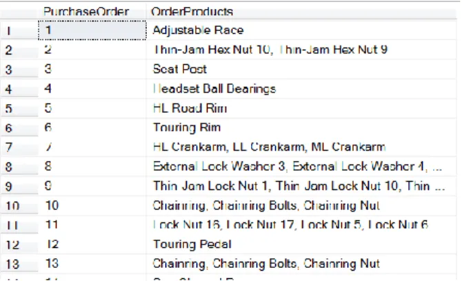
We now have all the pieces we need to produce results analogous to those in Figure 1. In the outer query, we simply need to include the purchase order’s ID. Listing 11 shows the query and Figure 2 shows part of the result, as displayed in SQL Server Management Studio (SSMS).
Listing 11. Combining the query from Listing 10 with code to include the purchase order number gives us the desired results.
SELECT PurchaseOrderID,
STUFF((SELECT ', ' + Name FROM (SELECT DISTINCT Name FROM Production.Product
Inner Join Purchasing.PurchaseOrderDetail As A On Production.Product.ProductID = A.ProductID
WHERE Purchasing.PurchaseOrderDetail.PurchaseOrderID = A.PurchaseOrderID) DistName ORDER BY Name
FOR XML PATH('')), 1, 2, '') OrderProducts FROM Purchasing.PurchaseOrderDetail
GROUP BY PurchaseOrderID ORDER BY 1
Figure 2. The query in Listing 11 produces this result.
This solution is included in the materials for this session as RollupOrdersForXML.sql.
Using a function
The second approach to producing the desired list uses a function that consolidates the list of products. The downside of this approach is that you either have to have the function in the database, or create it on the fly and then drop it afterward. If you need the comma-separated list of products regularly, of course, there’s really no reason not to add the function to the database.
The secret here is that the function accumulates the list in a variable, which it then returns to the main query. VFP doesn’t allow you to store query results to a variable, but SQL Server does, using the syntax in Listing 12. You can even assign results to multiple variables in a single query. The variables must be declared before the query.
Listing 12. SQL Server lets you store a query result into a variable.
SELECT @VarName = <expression> FROM <rest of query>
To create the comma-separated list, the expression on the right-hand side of the equal sign references the variable on the left-hand side. The code in Listing 13 shows how to do this for a single purchase order. To display the results in SSMS, add SELECT @Products at the end of the code block.
Listing 13. The ability to store a query result in a variable provides a way to accumulate the list of products for a single purchase order.
DECLARE @Products VARCHAR(1000)
SELECT @Products = COALESCE(@Products + ',', '') + Name FROM Production.Product
Inner Join Purchasing.PurchaseOrderDetail As A On Production.Product.ProductID = A.ProductID WHERE A.PurchaseOrderID = 7
The COALESCE() function accepts a list of expressions and returns the first one with a non-null value. Since @Products is initially non-null (because it’s not given an initial value), on the first record, COALESCE() chooses the empty string and the result doesn’t have a leading comma.
As in the FOR XML PATH case, the query here doesn’t remove duplicates. The solution is the same here; use a derived query to produce the list of distinct products before
combining them. (In this case, you need the derived table; there’s not a way to collect distinct product names without it.) Listing 14 shows the code that produces a sorted list of distinct products for one purchase order.
Listing 14. To include each product only once in the list, we again use a derived query inside the query that assembles the comma-separated list.
DECLARE @Products VARCHAR(1000)
SELECT @Products = COALESCE(@Products + ',', '') + Name FROM (SELECT DISTINCT Name
FROM Production.Product
Inner Join Purchasing.PurchaseOrderDetail As A On Production.Product.ProductID = A.ProductID WHERE A.PurchaseOrderID = 4008) DistNames
ORDER BY Name
We can use this code in a function to return the rolled-up list for a single purchase order. The main query calls the function for each purchase order. Listing 15 shows the full code for this solution. Note that it creates the function, uses it and then drops it. As noted earlier, if you’re going to do this regularly, just create the function once and keep it.
Listing 15. This solution to getting a comma-separated list of values from multiple records uses a function that rolls up the products for a single order.
CREATE FUNCTION ProductList (@POId INT) RETURNS VARCHAR(1000)
AS BEGIN
DECLARE @Products VARCHAR(1000)
SELECT @Products = COALESCE(@Products + ',', '') + Name FROM (SELECT DISTINCT Name
FROM Production.Product
Inner Join Purchasing.PurchaseOrderDetail As A On Production.Product.ProductID = A.ProductID WHERE A.PurchaseOrderID = @POId) DistNames ORDER BY Name
RETURN @Products END
go
SELECT DISTINCT PurchaseOrderID, dbo.productList(PurchaseOrderID) AS ProductList
FROM Purchasing.PurchaseOrderDetail go
DROP FUNCTION dbo.ProductList GO
Using DISTINCT in the main query ensures that we see each purchase order only once; otherwise, each would appear once for each included product.
This solution is included in the materials for this session as RollupOrdersByFunction.sql.
Which one?
Given two solutions, which one should you use? In my tests, the FOR XML PATH solution seems to be faster. However, the dataset in AdventureWorks is fairly small, so may not provide a good test bed. I recommend testing both solutions against your actual data. If you find no significant difference in execution, then use the one that you find easier to read and comprehend, since you’re likely to have to revisit it at some point.
Handle self-referential hierarchies
Relational databases handle typical hierarchical relationships very well. When you have something like customers, who place orders, which contain line items, representing products sold, any relational database should do. You create one table for each type of object and link them together with foreign keys.
Reporting on such data is easy, too. Fairly simple SQL queries let you collect the data you want with a few joins and some filters.
But some types of data don’t lend themselves to this sort of model. For example, the organization chart for a company contains only people, with some people managed by other people, who might in turn be managed by other people. Clearly, records for all people should be contained in a single table.
But how do you represent the manager relationship? One commonly used approach is to add a field to the person’s record that points to the record (in the same table) for his or her manager.
From a data-modeling point of view, this is a simple solution. However, reporting on such data can be complex. How do you trace the hierarchy from a given employee through her manager to the manager’s manager and so on up the chain of command? Given a manager, how do you find everyone who ultimately reports to that person (that is, reports to the person directly, or to someone managed by that person, or to someone managed by someone who is managed by that person, and so on down the line)?
Well look at two approaches to dealing with this kind of data, and show how much easier it is to get what you want in SQL Server than in VFP.
The traditional solution
As described above, the traditional way to handle this type of hierarchy is to add a field to identify a record’s parent (such as an employee’s manager). For example, the Northwind database has a field in the Employees table called ReportsTo. It contains the primary key of the employee’s manager; since that’s also a record in Employees, the table is
self-referential.
The AdventureWorks 2008 sample database for SQL Server doesn’t have this kind of relationship because it uses the second approach to hierarchies, discussed in “Using the HierarchyID type,” later in this paper. However, the 2005 version of the database has a set-up quite similar to the one in Northwind. The Employee table has a ManagerID field that contains the primary key (in Employee) of the employee’s manager.
Using the VFP Northwind and SQL Server AdventureWorks 2005 databases, let’s try to answer some standard questions about an organization chart.
Who manages an employee?
In both cases, determining the manager of an individual employee is quite simple. It just requires a self-join of the Employee table. That is, you use two instances of the Employee table, one to get the employee and one to get the manager. Listing 16 (EmpPlusMgr.PRG in the materials for this session) shows the VFP version of the query that retrieves this data for a single employee (by specifying the employee’s primary key; 4, in this case).
Listing 16. Use a self-join to connect an employee with his or her manager.
SELECT Emp.FirstName AS EmpFirst, ; Emp.LastName AS EmpLast, ; Mgr.FirstName AS MgrFirst, ; Mgr.LastName AS MgrLast ; FROM Employees Emp ;
JOIN Employees Mgr ;
ON Emp.ReportsTo = Mgr.EmployeeID ; WHERE Emp.EmployeeID = 4 ;
INTO CURSOR csrEmpAndMgr
The AdventureWorks version of the same task is a little more complex, because the database has a separate table for people (called Contact). The Employee table uses a
foreign key to Contact to identify the individual; Employee contains only the data related to employment. So extracting an employee’s name requires joining Employee to Contact. The solution still uses a self-join on the Employee table, but now it also requires two instances of the Contact table. Listing 17 (EmpPlusMgr.SQL in the materials for this session) shows the SQL Server query to retrieve the employee’s name and his or her manager’s name. Again, we retrieve data for a single employee (by specifying
Listing 17. The SQL Server version of the query is a little more complex, due to additional normalization, but still uses a self-join.
SELECT EmpContact.FirstName AS EmpFirst, EmpContact.LastName AS EmpLast, MgrContact.FirstName AS MgrFirst, MgrContact.LastName AS MgrLast FROM Person.Contact EmpContact
JOIN HumanResources.Employee Emp
ON Emp.ContactID = EmpContact.ContactID JOIN HumanResources.Employee Mgr
ON Emp.ManagerID = Mgr.EmployeeID JOIN Person.Contact MgrContact
ON Mgr.ContactID = MgrContact.ContactID WHERE Emp.EmployeeID = 37
It’s easy to extend these queries to retrieve the names of all employees with each one’s manager. Just remove the WHERE clause from each query.
What’s the management hierarchy for an employee?
Things start to get more interesting when you want to trace the whole management hierarchy for an employee. That is, given a particular employee, retrieve the name of her manager and of the manager’s manager and of the manager’s manager’s manager and so on up the line until you reach the person in charge.
Since we don’t know how many levels we might have, rather than putting all the data into a single record, here we create a cursor with one record for each level. The specified
employee comes first, and then we climb the hierarchy so that the big boss is last.
VFP’s SQL alone doesn’t offer a solution for this problem. Instead, you need to combine a little bit of SQL with some Xbase code, as in Listing 18. (This program is included in the materials for this session as EmpHierarchy.PRG.)
Listing 18. To track a hierarchy to the top in VFP calls for a mix of SQL and Xbase code.
* Start with a single employee and create a * hierarchy up to the top dog.
LPARAMETERS iEmpID
LOCAL iCurrentID , iLevel
OPEN DATABASE HOME(2) + "Northwind\Northwind"
CREATE CURSOR EmpHierarchy ;
(cFirst C(15), cLast C(20) , iLevel I)
USE Employees IN 0 ORDER EmployeeID
iCurrentID = iEmpID iLevel = 1
SEEK iCurrentID IN Employees
INSERT INTO EmpHierarchy ;
VALUES (Employees.FirstName, ; Employees.LastName, ; m.iLevel) iCurrentID = Employees.ReportsTo iLevel = m.iLevel + 1 ENDDO USE IN Employees SELECT EmpHierarchy
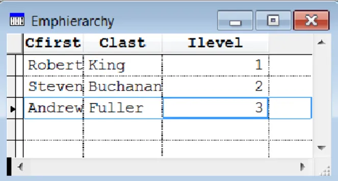
The strategy is to start with the employee you’re interested in, insert her data into the result cursor, then grab the PK for her manager and repeat until you reach an employee whose manager field is empty. Figure 3 shows the results when you pass 7 as the parameter.
Figure 3. Running the query in Listing 18, passing 7 as the parameter, gives these results.
SQL Server provides a simpler solution, by using a Common Table Expression (CTE). A CTE is a query that precedes the main query and provides a result that is then used in the main query. While similar to a derived table, CTEs have a couple of advantages.
First, the result can be included multiple times in the main query (with different aliases). A derived table is created in the FROM clause; if you need the same result again, you have to include the whole definition for the derived table again.
Second, and relevant to this problem, a CTE can have a recursive definition, referencing itself. That allows it to walk a hierarchy.
Listing 19 shows the structure of a query that uses a CTE. (It’s worth noting that a single query can have multiple CTEs; just separate them with commas.)
Listing 19. The definition for a CTE precedes the query that uses it.
WITH CTEAlias(Field1, Field2, ...) AS
SELECT <fieldlist> FROM <tables> ...
)
SELECT <main fieldlist> FROM <main query tables> ...
The query inside the parentheses is the CTE; its alias is whatever you specify in the WITH line. The WITH line also must contain a list of the fields in the CTE, though you don’t indicate their types or sizes.
The main query follows the parentheses and presumably includes the CTE in its list of tables and some of the CTE’s fields in the field list or the WHERE clause.
For example, the query in Listing 8 could instead use a CTE as in Listing 20, which is included in the materials for this session as SimpleCTE.SQL.
Listing 20. You can usually replace a derived table with a CTE.
WITH DistNames (Name) AS (SELECT DISTINCT Name FROM Production.Product
Inner Join Purchasing.PurchaseOrderDetail As A On Production.Product.ProductID = A.ProductID WHERE A.PurchaseOrderID = 4008) SELECT ', ' + Name FROM DistNames ORDER BY Name FOR XML PATH('')
For a recursive CTE, you combine two queries with UNION ALL. The first query is an "anchor"; it provides the starting record or records. The second query references the CTE itself to drill down recursively.
A recursive CTE continues drilling down until the recursive portion returns no records.
Listing 21 shows a query that produces the management hierarchy for the employee whose EmployeeID is 37. (Just change the assignment to @iEmpID to specify a different employee.) The query is included in the materials for this session as
EmpHierarchyViaCTE.SQL.
Listing 21. To retrieve the management hierarchy for an employee in the SQL Server AdventureWorks 2005 database, use a Common Table Expression.
DECLARE @iEmpID INT = 37;
WITH EmpHierarchy (
FirstName, LastName, ManagerID, EmpLevel) AS
SELECT Contact.FirstName, Contact.LastName, Employee.ManagerID, 1 AS EmpLevel FROM Person.Contact JOIN HumanResources.Employee ON Employee.ContactID = Contact.ContactID WHERE EmployeeID = @iEmpID UNION ALL
SELECT Contact.FirstName, Contact.LastName, Employee.ManagerID, EmpHierarchy.EmpLevel + 1 AS EmpLevel FROM Person.Contact JOIN HumanResources.Employee ON Employee.ContactID = Contact.ContactID JOIN EmpHierarchy ON Employee.EmployeeID = EmpHierarchy.ManagerID )
SELECT FirstName, LastName, EmpLevel FROM EmpHierarchy
The alias for the CTE here is EmpHierarchy. The anchor portion of the CTE selects the specified person (WHERE EmployeeID = @iEmpID), including that person’s ManagerID in the result and setting up a field to track the level in the database.
The recursive portion of the query joins the Employee table to the EmpHierarchy table-in-progress (that is, the CTE itself), matching the ManagerID from EmpHierarchy to
Employee.EmployeeID. It also increments the EmpLevel field, so that the first time it executes, EmpLevel is 2, the second time, it’s 3, and so forth.
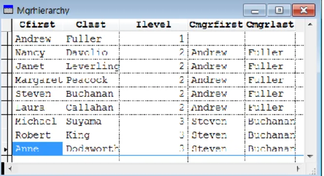
Once the CTE is complete, the main query pulls the desired information from it. Figure 4
shows the result of the query in Listing 21.
Figure 4. The query in Listing 21 returns one record for each level of the management hierarchy for the specified employee.
Who does an employee manage?
The problem gets a little tougher, at least on the VFP side, when we want to put together a list of all employees a particular person manages at all levels of the hierarchy. That is, not only those she manages directly, but people who report to those people, and so on down the line.
To make the results more meaningful, we want to include the name of the employee’s direct manager in the results.
What makes this difficult in VFP is that at each level, we may (probably do) have multiple employees. We need not only to add each to the result, but to check who each of them manages. That means we need some way of keeping track of who we’ve checked and who we haven’t.
We use two cursors. One (MgrHierarchy) holds the results, while the other
(EmpsToProcess) holds the list of people to check. Listing 22 shows the code; it’s called MgrHierarchy.PRG in the materials for this session.
Listing 22. Putting together the list of people a specified person manages directly or indirectly is harder than climbing up the hierarchy.
* Start with a single employee and determine * all the people that employee manages, * directly or indirectly.
LPARAMETERS iEmpID
LOCAL iCurrentID, iLevel, cFirst, cLast, LOCAL nCurRecNo, cMgrFirst, cMgrLast
OPEN DATABASE HOME(2) + "Northwind\Northwind"
CREATE CURSOR MgrHierarchy ;
(cFirst C(15), cLast C(20), iLevel I, ; cMgrFirst C(15), cMgrLast C(15)) CREATE CURSOR EmpsToProcess ;
(EmployeeID I, cFirst C(15), cLast C(20), ; iLevel I, cMgrFirst C(15), cMgrLast C(15))
INSERT INTO EmpsToProcess ;
SELECT m.iEmpID, FirstName, LastName, 1, "", "" ; FROM Employees ;
WHERE EmployeeID = m.iEmpID SELECT EmpsToProcess SCAN iCurrentID = EmpsToProcess.EmployeeID iLevel = EmpsToProcess.iLevel cFirst = EmpsToProcess.cFirst cLast = EmpsToProcess.cLast cMgrFirst = EmpsToProcess.cMgrFirst cMgrLast = EmpsToProcess.cMgrLast
* Insert this records into result INSERT INTO MgrHierarchy ;
VALUES (m.cFirst, m.cLast, m.iLevel, m.cMgrFirst, m.cMgrLast)
* Grab the current record pointer nCurRecNo = RECNO("EmpsToProcess")
INSERT INTO EmpsToProcess ;
FROM Employees ;
WHERE ReportsTo = m.iCurrentID
* Restore record pointer
GO m.nCurRecNo IN EmpsToProcess ENDSCAN
SELECT MgrHierarchy
To kick the process off, we add a single record to EmpsToProcess, with information about the specified employee. Then, we loop through EmpsToProcess, handling one employee at a time. We insert a record into MgrHierarchy for that employee, and then we add records to EmpsToProcess for everyone directly managed by the employee we’re now processing. The most interesting bit of this code is that the SCAN loop has no problem with the cursor we’re scanning growing as we go. We just have to keep track of the record pointer, and after adding records, move it back to the record we’re currently processing.
Figure 5 shows the result cursor when you pass 2 as the employee ID.
Figure 5. When you specify an EmployeeID of 2, you get all the Northwind employees.
In fact, you can do this with a single cursor that represents both the results and the list of people yet to check, but doing so makes the code a little confusing.
In SQL Server, solving this problem is no harder than solving the upward hierarchy. Again, we use a CTE, and all that really changes is the join condition in the recursive part of the CTE. (Because we want the direct manager’s name, the field list is slightly different, as well). Listing 23 shows the query (MgrHierarchyViaCTE.SQL in the materials for this session), along with a variable declaration to indicate which employee we want to start with; Figure 6 shows the results for this example.
Listing 23. Walking down the hierarchy of employees is no harder in SQL Server than climbing up.
DECLARE @iEmpID INT = 3;
WITH EmpHierarchy
(FirstName, LastName, EmployeeID, EmpLevel, MgrFirst, MgrLast) AS
SELECT Contact.FirstName, Contact.LastName, Employee.EmployeeID, 1 AS EmpLevel, CAST('' AS NVARCHAR(50)) AS MgrFirst CAST('' AS NVARCHAR(50)) AS MgrLast FROM Person.Contact
JOIN HumanResources.Employee
ON Employee.ContactID = Contact.ContactID WHERE EmployeeID = @iEmpID
UNION ALL
SELECT Contact.FirstName, Contact.LastName, Employee.EmployeeID, EmpHierarchy.EmpLevel + 1 AS EmpLevel, EmpHierarchy.FirstName AS MgrFirst, EmpHierarchy.LastName AS MgrLast FROM Person.Contact JOIN HumanResources.Employee ON Employee.ContactID = Contact.ContactID JOIN EmpHierarchy ON Employee.ManagerID = EmpHierarchy.EmployeeID )
SELECT FirstName, LastName, EmpLevel, MgrFirst, MgrLast
FROM EmpHierarchy
Figure 6. These are the people managed by Roberto Tamburello, whose EmployeeID is 3.
Using the HierarchyID type
SQL Server 2008 introduced a new way to handle this kind of hierarchy. A new data type called HierarchyID encodes the path to any node in a hierarchy into a single field; a set of methods for the data type make both maintaining and navigating straightforward. (The idea of a data type with methods is unusual. Think of the data type as essentially a class that you can use as a field.)
The SQL Server 2008 version of AdventureWorks uses the HierarchyID type to handle the management hierarchy (which is why we couldn’t use it for the earlier examples). There are other changes, as well. AdventureWorks 2008 is even more normalized than the 2005
version; a new BusinessEntity table contains information about people (including employees) and businesses. So, instead of an EmployeeID, each employee now has a BusinessEntityID. In addition, the Contact table has been renamed Person. However, there’s still a relationship between that table and the Employee table that we can use to retrieve an employee’s name.
HierarchyID essentially creates a string that shows the path from the root (top) of the hierarchy to a particular record. The root node is indicated as "/"; then, at each level, a number indicates which child of the preceding node is in this node’s hierarchy. So, for example, a hierachyID of "/4/3/" means that the node is descended from the fourth child of the root node, and is the third child of that child. However, HierarchyIDs are actually stored in a binary string created from the plain text version.
The HierarchyID type has a set of methods that allow you to easily navigate the hierarchy. First, the ToString method converts the encoded hierarchy ID to a string in the form shown above. Listing 24 (ShowHierarchyID.SQL in the materials for this session) shows a query to extract the name and hierarchy ID, both in encoded and plain text form, of the
AdventureWorks employees; Figure 7 shows a portion of the result.
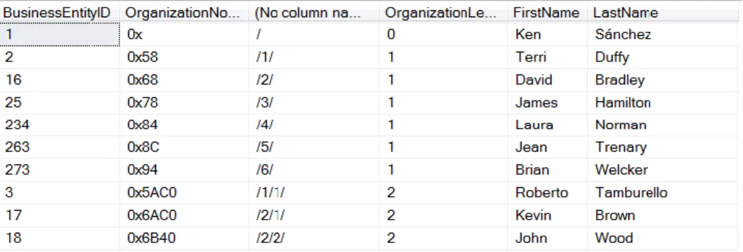
Listing 24.The ToString method of the HierarchyID type converts the hierarchy ID into a human-readable form. SELECT Person.[BusinessEntityID] ,[OrganizationNode] ,[OrganizationNode].ToString() ,[OrganizationLevel] , FirstName , LastName FROM [HumanResources].[Employee] JOIN Person.Person ON Employee.BusinessEntityID = Person.BusinessEntityID
Figure 7. The unnamed column here shows the text version of the OrganizationNode column.
To move through the hierarchy, we use the GetAncestor method. As you’d expect, GetAncestor returns an ancestor of the node you apply it to. A parameter indicates how many levels up the hierarchy to go, so GetAncestor(1) returns the parent of the node.
That’s actually all we need to retrieve the management hierarchy for a particular employee. As in the earlier example, we use a CTE to handle the recursive requirement. Listing 25
shows the query; it’s included in the materials for this session as EmpHierarchyWithHierarchyID.SQL.
Listing 25. Retrieving the management hierarchy for a given employee when using the HierarchyID data type isn’t much different from doing it with a "reports to" field.
DECLARE @iEmpID INT = 40;
WITH EmpHierarchy (FirstName, LastName, OrganizationNode, EmpLevel) AS
(
SELECT Person.FirstName, Person.LastName, Employee.OrganizationNode, 1 AS EmpLevel FROM Person.Person
JOIN HumanResources.Employee
ON Employee.BusinessEntityID = Person.BusinessEntityID WHERE Employee.BusinessEntityID = @iEmpID
UNION ALL
SELECT Person.FirstName, Person.LastName,
Employee.OrganizationNode, EmpHierarchy.EmpLevel + 1 AS EmpLevel FROM Person.Person JOIN HumanResources.Employee ON Employee.BusinessEntityID = Person.BusinessEntityID JOIN EmpHierarchy ON Employee.OrganizationNode = EmpHierarchy.OrganizationNode.GetAncestor(1) )
SELECT FirstName, LastName, EmpLevel FROM EmpHierarchy
The big difference between this query and the earlier query is in the join between
Employee and EmpHierarchy. Rather than matching fields directly, we call GetAncestor to retrieve the hierarchy for a node’s parent and compare that to the Employee table’s OrganizationNode field.
As in the earlier examples, finding everyone an employee manages uses a very similar query, but in the join condition between Employee and EmpHierarchy, we apply
GetAncestor to the field from Employee. Listing 26 (MgrHierarchyWithHierarchyID.SQL in the materials for this session) shows the code.
Listing 26. To find everyone an individual manages using HierarchyID, just change the direction of the join between Employee and EmpHierarchy.
DECLARE @iEmpID INT = 3;
WITH EmpHierarchy
(FirstName, LastName, BusinessEntityID, EmpLevel, MgrFirst, MgrLast, OrgNode) AS
SELECT Person.FirstName, Person.LastName,
Employee.BusinessEntityID, 1 AS EmpLevel, CAST('' AS NVARCHAR(50)) AS MgrFirst, CAST('' AS NVARCHAR(50)) AS MgrLast, OrganizationNode AS OrgNode
FROM Person.Person
JOIN HumanResources.Employee
ON Employee.BusinessEntityID = Person.BusinessEntityID WHERE Employee.BusinessEntityID = @iEmpID
UNION ALL
SELECT Person.FirstName, Person.LastName, Employee.BusinessEntityID, EmpHierarchy.EmpLevel + 1 AS EmpLevel, EmpHierarchy.FirstName AS MgrFirst, EmpHierarchy.LastName AS MgrLast, OrganizationNode AS OrgNode FROM Person.Person JOIN HumanResources.Employee ON Employee.BusinessEntityID = Person.BusinessEntityID JOIN EmpHierarchy ON Employee.OrganizationNode.GetAncestor(1) = EmpHierarchy.OrgNode )
SELECT FirstName, LastName, EmpLevel, MgrFirst, MgrLast FROM EmpHierarchy
Setting up HierarchyIDs
Populating a HierarchyID field turns out to be simple. You can specify the plain text version and SQL Server will handle encoding it. You can also use the GetRoot and GetDescendant methods to populate the field.
GetDescendant is particularly useful for inserting a child of an existing record. You call the GetDescendant method of the parent record, passing parameters that indicate where the new record goes among the children of the parent. A complete explanation of the method is beyond the scope of this article, but Listing 27 shows code that creates a temporary table and adds a few records, and then shows the results. This code is included in the materials for this session as CreateHierarchy.SQL.
Listing 27. You can specify the hierarchyID value directly or use the GetRoot and GetDescendant methods.
CREATE TABLE #temp
(orgHier HIERARCHYID, NodeName CHAR(20))
INSERT INTO #temp
( orgHier, NodeName ) VALUES ( '/', 'Root') )
DECLARE @Root HIERARCHYID, @curNode HIERARCHYID
SELECT @Root = hierarchyID::GetRoot()
( orgHier, NodeName )
VALUES ( @Root.GetDescendant(NULL, NULL), 'First child' )
SELECT @curNode = MAX(orgHier) FROM #temp
WHERE orgHier.GetAncestor(1) = @Root
INSERT INTO #temp
( orgHier, NodeName )
VALUES ( @curNode.GetDescendant(NULL, NULL), 'First grandchild')
INSERT INTO #temp
( orgHier, NodeName )
VALUES ( @Root.GetDescendant(@curNode, NULL), 'Second child')
SELECT orgHier, orgHier.ToString(), NodeName
FROM #temp
DROP TABLE #temp
You’ll find a good tutorial on the HierarchyID type, including a discussion of the methods, at http://tinyurl.com/n6kk6jm.
What about VFP?
Obviously, VFP has no analogue of the HierarchyID data type. However, you can create your own. Marcia Akins describes an approach to doing so in her paper "Modeling Hierachies," available at http://tightlinecomputers.com/Downloads.htm; scroll down near the bottom of the page.
Of course, a home-grown version won’t include the methods that SQL Server’s HierarchyID type comes with. You’ll have to write your own code to handle look-ups and insertions.
Get the top N from each group
Both VFP and SQL Server include the TOP n clause, which allows you to include in the result only the first n records that match a query’s filter conditions. But TOP n doesn’t work when what you really want is the TOP n for each group in the query.
Suppose a company wants to know its top five salespeople for each year in some period. In VFP, you need to combine SQL with Xbase code or use a trick to get the desired results. With SQL Server, you can do it with a single query.
The VFP solution
Collecting the basic data you need to solve this problem is straightforward. Listing 28
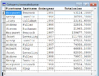
(EmployeeSalesByYear.PRG in the materials for this session) shows a query that provides each employee’s sales by year; Figure 8 shows part of the results.
Listing 28. Getting total sales by employee by year is easy in VFP.
SELECT FirstName, LastName, ;
YEAR(OrderDate) as OrderYear, ; SUM(UnitPrice*Quantity) AS TotalSales ; FROM Employees ; JOIN Orders ; ON Employees.EmployeeID = Orders.EmployeeID ; JOIN OrderDetails ; ON Orders.OrderID = OrderDetails.OrderID ; GROUP BY 1, 2, 3 ;
ORDER BY OrderYear, TotalSales DESC ; INTO CURSOR csrEmployeeSalesByYear
Figure 8. The query in Listing 28 produces the total sales for each employee by year.
However, when you want to keep only the top five for each year, you need to either combine SQL code with some Xbase code or use a trick that can result in a significant slowdown with large datasets.
SQL plus Xbase
The mixed solution is easier to follow, so let’s start with that one. The idea is to first select the raw data needed, in this case, the total sales by employee by year. Then we loop
through on the grouping field, and select the top n (five, in this case) in each group and put them into a cursor. Listing 29 (TopnEmployeeSalesByYear-Loop.PRG in the materials for this session) shows the code; Figure 9 shows the result.
Listing 29. One way to find the top n in each group is to collect the data, then loop through it by group.
SELECT EmployeeID, ; YEAR(OrderDate) as OrderYear, ; SUM(UnitPrice*Quantity) AS TotalSales ; FROM Orders ; JOIN OrderDetails ; ON Orders.OrderID = OrderDetails.OrderID ; GROUP BY 1, 2 ;
INTO CURSOR csrEmpSalesByYear
CREATE CURSOR csrTopEmployeeSalesByYear ; (FirstName C(10), LastName C(20), ; OrderYear N(4), TotalSales Y)
SELECT distinct OrderYear ; FROM csrEmpSalesByYear ; INTO CURSOR csrYears LOCAL nYear SCAN nYear = csrYears.OrderYear
INSERT INTO csrTopEmployeeSalesByYear ; SELECT TOP 5 ; FirstName, LastName, ; OrderYear, TotalSales ; FROM Employees ; JOIN csrEmpSalesByYear ; ON Employees.EmployeeID = csrEmpSalesByYear.EmployeeID ; WHERE csrEmpSalesByYear.OrderYear = m.nYear ;
ORDER BY OrderYear, TotalSales DESC
ENDSCAN
USE IN csrYears
USE IN csrEmpSalesByYear
SELECT csrTopEmployeeSalesByYear
Figure 9. The query in Listing 29 produces these results.
The first query is just a simpler version of Listing 28, omitting the Employees table and the ORDER BY clause; both of those will be used later. Next, we create a cursor to hold the final results. Then, we get a list of the years for which we have data. Finally, we loop through the cursor of years and, for each, grab the top five salespeople for that year, and put them into the result cursor, adding the employee’s name and sorting as we insert.
You can actually consolidate this version a little by turning the first query into a derived table in the query inside the INSERT command. Listing 30 (TopnEmployeeSalesByYear-Loop2.PRG in the materials for this session) shows the revised version. Note that you have
to get the list of years directly from the Orders table in this version. This version, of course, gives the same results.
Listing 30. The code in Listing 29 can be reworked to use a derived table to compute the totals for each year.
CREATE CURSOR csrTopEmployeeSalesByYear ; (FirstName C(10), LastName C(20), ; OrderYear N(4), TotalSales Y)
SELECT distinct YEAR(OrderDate) AS OrderYear ; FROM Orders ;
INTO CURSOR csrYears LOCAL nYear SCAN nYear = csrYears.OrderYear
INSERT INTO csrTopEmployeeSalesByYear ; SELECT TOP 5 ; FirstName, LastName, ; OrderYear, TotalSales ; FROM Employees ; JOIN ( ; SELECT EmployeeID, ; YEAR(OrderDate) as OrderYear, ; SUM(UnitPrice * Quantity) ; AS TotalSales ; FROM Orders ; JOIN OrderDetails ; ON Orders.OrderID = OrderDetails.OrderID ; WHERE YEAR(OrderDate) = m.nYear ;
GROUP BY 1, 2) csrEmpSalesByYear ;
ON Employees.EmployeeID = csrEmpSalesByYear.EmployeeID ; ORDER BY OrderYear, TotalSales DESC
ENDSCAN
USE IN csrYears
SELECT csrTopEmployeeSalesByYear
SQL-only
The alternative VFP solution uses only SQL commands, but relies on a trick of sorts. Like the mixed solution, it starts with a query to collect the basic data needed. It then joins that data to itself in a way that results in multiple records for each employee/year combination and uses HAVING to keep only those that represent the top n records. Finally, it adds the employee name. Listing 31 (TopNEmployeeSalesByYear-Trick.prg in the materials for this session) shows the code.
Listing 31. This solution uses only SQL, but requires a tricky join condition. SELECT EmployeeID, ; YEAR(OrderDate) as OrderYear, ; SUM(UnitPrice * Quantity) ; AS TotalSales ; FROM Orders ; JOIN OrderDetails ; ON Orders.OrderID = OrderDetails.OrderID ; GROUP BY 1, 2 ;
INTO CURSOR csrEmpSalesByYear
SELECT FirstName, LastName, ; OrderYear, TotalSales ; FROM Employees ; JOIN ( ; SELECT ESBY1.EmployeeID, ; ESBY1.OrderYear, ; ESBY1.TotalSales ;
FROM csrEmpSalesByYear ESBY1 ; JOIN csrEmpSalesByYear ESBY2 ;
ON ESBY1.OrderYear = ESBY2.OrderYear ; AND ESBY1.TotalSales <= ESBY2.TotalSales ; GROUP BY 1, 2,3 ;
HAVING COUNT(*) <= 5) csrTop5;
ON Employees.EmployeeID = csrTop5.EmployeeID ; ORDER BY OrderYear, TotalSales DESC ;
INTO CURSOR csrTopEmployeeSalesByYear
The first query here is just a variant of Listing 28. The key portion of this approach is the derived table in the second query, in particular, the join condition between the two instances of csrEmpSalesByYear, shown in Listing 32. Records are matched up first by having the same year and then by having sales in the second instance be the same or more than sales in the first instance. This results in a single record for the employee from that year with the highest sales total, two records for the employee with the second highest sales total and so on.
Listing 32. The key to this solution is the unorthodox join condition between two instances of the same table.
FROM csrEmpSalesByYear ESBY1 ; JOIN csrEmpSalesByYear ESBY2 ;
ON ESBY1.OrderYear = ESBY2.OrderYear ; AND ESBY1.TotalSales <= ESBY2.TotalSales
The GROUP BY and HAVING clauses then combine all the records for a given employee and year, and keeps only those where the number of records in the intermediate result is five or fewer (that is, where the count of records in the group is five or less), providing the top five salespeople for each year.
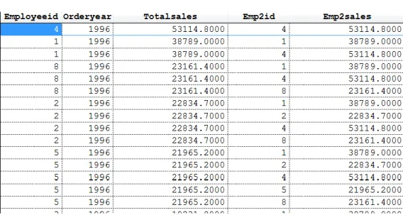
To make more sense of this solution, first consider the query in Listing 33 (included in the materials for this session as TopNEmployeeSalesByYearBeforeGrouping.prg). It assumes we’ve already run the query to create the EmpSalesByYear cursor. It shows the results
(plus a couple of additional fields) from the derived table in Listing 31 before the GROUP BY is applied. In the partial results shown in Figure 10, you can see one record for
employee 4 in 1996, two for employee 1, three for employee 8 and so forth. The added columns Emp2ID and Emp2Sales show which row in ESBY2 resulted in this result row. So, for employee 4 in 1996, the only row that met the conditions was the one for employee 4 in 1996. For employee 1 in 1996, both employee 4 and itself met the conditions of total sales the same or more than his or her own.
Listing 33. This query demonstrates the intermediate results for the derived table in Listing 31.
SELECT ESBY1.EmployeeID, ; ESBY1.OrderYear, ; ESBY1.TotalSales , ;
ESBY2.EmployeeID AS Emp2ID, ; ESBY2.TotalSales AS Emp2Sales ; FROM EmpSalesByYear ESBY1 ;
JOIN EmpSalesByYear ESBY2 ;
ON ESBY1.OrderYear = ESBY2.OrderYear ; AND ESBY1.TotalSales <= ESBY2.TotalSales ; ORDER BY ESBY1.OrderYear, ESBY1.TotalSales DESC ; INTO CURSOR csrIntermediate
Figure 10. The query in Listing 33 unfolds the data that’s grouped in the derived table.
The problem with this approach to the problem is that, as the size of the original data increases, it can get bogged down. So while this solution has a certain elegance, in the long run, a SQL plus Xbase solution is probably a better choice.
By the way, this example (the one in Listing 31) shows where CTEs (common table expressions, explained earlier in this paper) would be useful in VFP’s SQL. We can’t easily combine the two queries into one because the second query uses two instances of the EmpSalesByYear. If VFP supported CTEs, we could make the query that creates EmpSalesByYear into a CTE, and then use it twice in the main query.
The SQL Server solution
Solving the top n by group problem in SQL Server uses a couple of CTEs, but also uses another construct that’s not available in VFP’s version of SQL.
The OVER clause lets you apply a function to all or part of a result set; it’s used in the field list. There are several variations, but the basic structure is shown in Listing 34.
Listing 34. The OVER clause lets you apply a function to all or some of the records in a query.
<function> OVER (<grouping and/or ordering>)
OVER lets you rank records, as well as applying aggregates to individual items in the field list. In SQL Server 2012 and later, OVER has additional features that let you compute complicated aggregates such as running totals and moving averages.
For the top n by group problem, we want to rank records within a group and then keep the top n. To do that, we can use the ROW_NUMBER() function, which , as its name suggests, returns the row number of a record within a group (or within the entire result set, if no grouping is specified).
For example, Listing 35 (included in the materials for this session as
EmployeeOrderNumber.sql) shows a query that lists AdventureWorks (2008) employees in the order they were hired, giving each an "employee order number." Here, the data is ordered by HireDate and then ROW_NUMBER() is applied to provide the position of each record. Figure 11 shows partial results.
Listing 35. Using ROW_NUMBER() with OVER lets you give records a rank.
SELECT FirstName, LastName, HireDate, ROW_NUMBER() OVER (ORDER BY HireDate) AS EmployeeOrderNumber
FROM HumanResources.Employee JOIN Person.Person
Figure 11. The query in Listing 35 applies a rank to each employee by hire date.
But look at Ruth Ellerbock and Gail Erickson; they have the same hire date, but different values for EmployeeOrderNumber. Sometimes, that’s what you want, but sometimes, you want such records to have the same value.
The ROW_NUMBER() funtion doesn’t know anything about ties. However, the RANK() function is aware of ties and assigns them the same value, then skips the appropriate number of values. Listing 36 (EmployeeRank.SQL in the materials for this session) shows the same query using RANK() instead of ROW_NUMBER(); Figure 12 shows the first few records. This time, you can see that Ellerbock and Erickson have the same rank, 8, while Barry Johnson, who immediately follows them, still has a rank of 10.
Listing 36. The RANK() function is aware of ties, assigning them the same value.
SELECT FirstName, LastName, HireDate, RANK() OVER (ORDER BY HireDate) AS EmployeeOrderNumber
FROM HumanResources.Employee JOIN Person.Person
Figure 12. Using RANK() assigns the same EmployeeOrderNumber to records with the same hire date.
You can’t say that either ROW_NUMBER() or RANK() is right; which one you want depends on the situation. In fact, there’s a third related function, DENSE_RANK() that behaves like RANK(), giving ties the same value, but then continues numbering in order. That is, if we used DENSE_RANK() in this example, Barry Johnson would have a rank of 9, rather than 10.
Partitioning with OVER
In addition to specifying ordering, OVER also allows us to divide the data into groups before applying the function, using the PARTITION BY clause. The query in Listing 37
(included in the materials for this session as EmployeeRankByDept.sql) assigns employee ranks within each department rather than for the company as a whole by using both PARTITION BY and ORDER BY. Figure 13 shows partial results; note that the numbering begins again for each department and that ties are assigned the same rank.
Listing 37. Combining PARTITION BY and ORDER BY in the OVER clause lets you apply ranks within a group.
SELECT FirstName, LastName, StartDate, Department.Name, RANK() OVER (PARTITION BY Department.DepartmentID ORDER BY StartDate) AS EmployeeRank FROM HumanResources.Employee JOIN HumanResources.EmployeeDepartmentHistory ON Employee.BusinessEntityID = EmployeeDepartmentHistory.BusinessEntityID JOIN HumanResources.Department ON EmployeeDepartmentHistory.DepartmentID = Department.DepartmentID JOIN Person.Person ON Employee.BusinessEntityID = Person.BusinessEntityID WHERE EndDate IS null
Figure 13. Here, employees are numbered within their current department, based on when they started in that department.
This example should provide a hint as to how we’ll solve the top n by group problem, since we now have a way to number things by group. All we need to do is filter so we only keep those whose rank within the group is in the range of interest. However, it’s not possible to filter on the computed field EmployeeOrderNumber in the same query. Instead, we turn that query into a CTE and filter in the main query, as in Listing 38
(LongestStandingEmployeesByDept.sql in the materials for this session).
Listing 38. Once we have the rank for an item within its group, we just need to filter to get the top n items by group.
WITH EmpRanksByDepartment AS
(SELECT FirstName, LastName, StartDate, Department.Name AS Department, RANK() OVER (PARTITION BY Department.DepartmentID ORDER BY StartDate) AS EmployeeRank FROM HumanResources.Employee JOIN HumanResources.EmployeeDepartmentHistory ON Employee.BusinessEntityID = EmployeeDepartmentHistory.BusinessEntityID JOIN HumanResources.Department ON EmployeeDepartmentHistory.DepartmentID = Department.DepartmentID JOIN Person.Person ON Employee.BusinessEntityID = Person.BusinessEntityID WHERE EndDate IS NULL)
SELECT FirstName, LastName, StartDate, Department FROM EmpRanksByDepartment
WHERE EmployeeRank <= 3
ORDER BY Department, StartDate
Figure 14 shows part of the result. Note that there are many more than three records for the Sales department because a whole group of people started on the same day. If you really want only three per department and don’t care which records you omit from a last-place tie, use RECORD_NUMBER() instead of RANK().
Figure 14. The query in Listing 38 provides the three longest-standing employees in each department. When there are ties, it may produce more than three results.
Applying the same principle to finding the top five salespeople by year at AdventureWorks (to match our VFP example) is a little more complicated because we have to compute sales totals first. To make that work, we first use a CTE to compute those totals and then a
second CTE based on that result to add the ranks. (Note the comma between the two CTEs.)
Listing 39 (TopSalesPeopleByYear.sql in the materials for this session) shows the complete query.
Listing 39. Finding the top five salepeople by year requires cascading CTEs, plus the OVER clause.
WITH TotalSalesBySalesPerson AS (SELECT BusinessEntityID, YEAR(OrderDate) AS nYear, SUM(SubTotal) AS TotalSales FROM Sales.SalesPerson JOIN Sales.SalesOrderHeader ON SalesPerson.BusinessEntityID = SalesOrderHeader.SalesPersonID GROUP BY BusinessEntityID, YEAR(OrderDate)),
RankSalesPerson AS
(SELECT BusinessEntityID, nYear, TotalSales, RANK() OVER
(PARTITION BY nYear
ORDER BY TotalSales DESC) AS nRank FROM TotalSalesBySalesPerson)
SELECT FirstName, LastName, nYear, TotalSales FROM RankSalesPerson
JOIN Person.Person
ON RankSalesPerson.BusinessEntityID = Person.BusinessEntityID WHERE nRank <= 5
The first CTE, TotalSalesBySalesPerson, contains the ID for the salesperson, the year and that person‘s total sales for the year. The second CTE, RankSalesPerson, adds rank within the group to the data from TotalSalesByPerson. Finally, the main query keeps only the top five in each and adds the actual name of the person. Figure 15 shows partial results.
Figure 15. These partial results show the top five salespeople by year.
It’s worth noting the very cool feature demonstrated by this query. Not only can a query have multiple CTEs, but CTEs later in the list can be based on previous CTEs. So
RankSalesPerson uses TotalSalesBySalesPerson in its FROM list.
The OVER clause has other uses, such as helping to de-dupe a list. In SQL 2012 and later, it’s even more useful, with the ability to apply the function to a group of records based not only on an expression, but based on position within a group.
Summarize aggregated data
As earlier sections of this paper show, SQL SELECT’s GROUP BY clause makes it easy to aggregate data in a query. Just include the fields that specify the groups and some fields using the aggregate functions (COUNT, SUM, AVG, MIN, MAX in VFP; SQL Server has those and a few more).
For example, the query in Listing 40 (TotalsByCountryCity.PRG in the materials for this session) fills a cursor with sales for each city for each month; Figure 16 shows partial results.
Listing 40. This query computes total sales for each combination of country, city, year and month.
SELECT Country, City, ;
YEAR(OrderDate) AS OrderYear, MONTH(OrderDate) AS OrderMonth, ; SUM(Quantity * OrderDetails.UnitPrice) AS nTotal ;
AVG(Quantity * OrderDetails.UnitPrice) AS nAvg, ; COUNT(*) AS nCount ; FROM Customers ; JOIN Orders ; ON Customers.CustomerID = Orders.CustomerID ; JOIN OrderDetails ; ON Orders.OrderID = OrderDetails.OrderID ; GROUP BY OrderYear, OrderMonth, ;
Country, City ; ORDER BY Country, City, ;
INTO CURSOR csrCtyTotals
Figure 16. The query in Listing 40 computes the total sales for each city in each month.
You can do an analogous query using the SQL Server AdventureWorks 2008 database, though it involves a lot more tables because the AdventureWorks database covers a wider range of data than just sales. Listing 41 (SalesByCountryCity.SQL in the materials for this session) shows the corresponding SQL Server query.
Listing 41. Aggregating the data with SQL Server’s AdventureWorks 2008 database is more verbose, but contains the same elements.
SELECT Person.CountryRegion.Name AS Country, Person.Address.City, YEAR(OrderDate) AS nYear, MONTH(OrderDate) AS nMonth, SUM(SubTotal) AS TotalSales AVG(SubTotal) AS AvgSale, COUNT(*) AS NumSales FROM Sales.Customer JOIN Person.Person ON Customer.PersonID = Person.BusinessEntityID JOIN Person.BusinessEntityAddress ON Person.BusinessEntityID = BusinessEntityAddress.BusinessEntityID JOIN Person.Address ON BusinessEntityAddress.AddressID = Address.AddressID JOIN Person.StateProvince ON Address.StateProvinceID = StateProvince.StateProvinceID JOIN Person.CountryRegion ON StateProvince.CountryRegionCode = CountryRegion.CountryRegionCode JOIN Sales.SalesOrderHeader ON Customer.CustomerID = SalesOrderHeader.CustomerID JOIN Sales.SalesOrderDetail ON SalesOrderHeader.SalesOrderID = SalesOrderDetail.SalesOrderID GROUP BY CountryRegion.Name, Address.City,
The rules for grouping are pretty simple. The field list contains two types of fields, those to group on, and those that are being aggregated. In the VFP example, the fields to group on are Country, City, OrderYear and OrderMonth, and the aggregated fields are nTotal, nAvg and nCount. The SQL Server query has the same list, but some of the field names are different. (Before VFP 8, you could include fields in the list that were neither grouped or nor aggregated, but doing so could give you misleading results. This article on my website explains the problem in detail: http://tinyurl.com/leydyqw.)
Computing group totals
What the basic query doesn’t give you, though, is aggregation (that is, summaries) at any level except the one you specify. That is, while you get the total, average and count for a specific city in a specific month, you don’t get them for that city for the whole year, or for that month for a whole country, and so on. Figure 17 shows what we’re looking for. At the end of each year, a new record shows the total, average and count for that year. At the end of each city, another record shows the city’s total, average and count and at the end of each country, yet another record has country-wide results.
Figure 17. It can be useful to have group totals in the same cursor as the original data.
In VFP, there are three ways to get that data. One is to create a report and use totals and report variables to compute and report that data, but of course, then you only have the data as output, not in a VFP cursor.
The second choice is to use Xbase code to compute them based on the initial cursor. Listing 42 (WithGroupTotalsXbase.PRG in the materials for this session) shows how to do this; it assumes you’ve already run the query in Listing 40. It keeps running totals and counts for
each level: year, city, country and overall. Then, when one of those changes, it inserts the appropriate record.
Listing 42. You can add subgroup aggregates by looping through the cursor.
LOCAL nYearTotal, nCityTotal, nCountryTotal, nGrandTotal LOCAL nYearCnt, nCityCnt, nCountryCount, nGrandCount LOCAL nCurYear, cCurCity, cCurCountry
* Create a new cursor to hold the results SELECT * ;
FROM csrCtyTotals ; WHERE .F. ;
INTO CURSOR csrWithGroupTotals READWRITE
SELECT csrCtyTotals
STORE 0 TO nYearTotal, nCityTotal, nCountryTotal, nGrandTotal STORE 0 TO nYearCount, nCityCount, nCountryCount, nGrandCount nCurYear = csrCtyTotals.OrderYear
cCurCity = csrCtyTotals.City cCurCountry = csrCtyTotals.Country
SCAN
* First check for end of year,
* but could be same year and change of city * or country.
IF csrCtyTotals.OrderYear <> m.nCurYear OR ; NOT (csrCtyTotals.City == m.cCurCity) OR; NOT (csrCtyTotals.Country == m.cCurCountry) INSERT INTO csrWithGroupTotals ;
VALUES (m.cCurCountry, m.cCurCity, ; m.nCurYear, .null., ;
m.nYearTotal, ;
m.nYearTotal/m.nYearCount, ; m.nYearCount)
m.nCurYear = csrCtyTotals.OrderYear STORE 0 TO m.nYearTotal, m.nYearCount
* Now check for change of city
IF NOT (csrCtyTotals.City == m.cCurCity) ;
OR NOT (csrCtyTotals.Country == m.cCurCountry) INSERT INTO csrWithGroupTotals ;
VALUES (m.cCurCountry, ; m.cCurCity, ; .null., .null., ; m.nCityTotal, ; m.nCityTotal/m.nCityCount, ; m.nCityCount) m.cCurCity = csrCtyTotals.City
STORE 0 TO m.nCityTotal, m.nCityCount
* Now check for change of country
IF NOT (csrCtyTotals.Country == m.cCurCountry) INSERT INTO csrWithGroupTotals ;
VALUES (m.cCurCountry, .null., ‚ .null., .null., ; m.nCountryTotal, ; m.nCountryTotal/m.nCountryCount, ; m.nCountryCount) m.cCurCountry = csrCtyTotals.Country STORE 0 TO m.nCountryTotal, m.CountryCount ENDIF
ENDIF ENDIF
* Now handle current record INSERT INTO csrWithGroupTotals ; VALUES (csrCtyTotals.Country, ; csrCtyTotals.City, ; csrCtyTotals.OrderYear, ; csrCtyTotals.OrderMonth, ; csrCtyTotals.nTotal, ; csrCtyTotals.nAvg, ; csrCtyTotals.nCount)
nYearTotal = m.nYearTotal + csrCtyTotals.nTotal nYearCount = m.nYearCount + csrCtyTotals.nCount nCityTotal = m.nCityTotal + csrCtyTotals.nTotal nCityCount = m.nCityCount + csrCtyTotals.nCount
nCountryTotal = m.nCountryTotal + csrCtyTotals.nTotal nCountryCount = m.nCountryCount + csrCtyTotals.nCount nGrandTotal = m.nGrandTotal + csrCtyTotals.nTotal nGrandCount = m.nGrandCount + csrCtyTotals.nCount
ENDSCAN
* Now insert grand totals
INSERT INTO csrWithGroupTotals ;
VALUES (.null., .null., .null., .null., ; m.nGrandTotal, ;
m.nGrandTotal/m.nGrandCount, ; m.nGrandCount)
The third choice is to do a series of queries, each grouping on different levels and then consolidate the results. Listing 43 shows this version of the code; as in the previous example, it assumes you’ve already run the query that creates csrCtyTotals. This code creates a cursor with each city’s annual totals, one with each city’s overall totals, one with each country’s overall totals, and one containing the grand total. Then it uses UNION to combine all the results into a single cursor. It’s included in the materials for this session as WithGroupTotalsSQL.PRG.
Listing 43. You can add the yearly, city-wide and country-wide totals using SQL, as well.
* Now year totals by city
SELECT Country, City, OrderYear, ; 999 as OrderMonth, ;
SUM(nTotal) AS nTotal, ;
SUM(nCount) AS nCount ; FROM csrCtyTotals ;
GROUP BY Country, City, OrderYear ; INTO CURSOR csrYearTotals
* Now city totals SELECT Country, City, ; 99999 AS OrderYear, ; 999 as OrderMonth, ; SUM(nTotal) AS nTotal, ; SUM(nTotal)/SUM(nCount) AS nAvg, ; SUM(nCount) AS nCount ; FROM csrCtyTotals ; GROUP BY Country, City ; INTO CURSOR csrCityTotals
* Now country totals SELECT Country, ; REPLICATE('Z', 15) AS City, ; 99999 AS OrderYear, ; 999 as OrderMonth, ; SUM(nTotal) AS nTotal, ; SUM(nTotal)/SUM(nCount) AS nAvg, ; SUM(nCount) AS nCount ; FROM csrCtyTotals ; GROUP BY Country ;
INTO CURSOR csrCountryTotals
* Now grand total
SELECT REPLICATE('Z', 15) AS Country, ; REPLICATE('Z', 15) AS City, ; 99999 AS OrderYear, ; 999 as OrderMonth, ; SUM(nTotal) AS nTotal, ; SUM(nTotal)/SUM(nCount) AS nAvg, ; SUM(nCount) AS nCount ; FROM csrCtyTotals ; INTO CURSOR csrGrandTotal
* Create one cursor SELECT * ; FROM csrCtyTotals ; UNION ALL ; SELECT * ; FROM csrYearTotals ; UNION ALL ; SELECT * ; FROM csrCityTotals ; UNION ALL ; SELECT * ; FROM csrCountryTotals ; UNION ALL ; SELECT * ; FROM csrGrandTotal ; ORDER BY Country, City, ;