Modeling green cyclic inventory routing problem with multiple objectives using discrete particle swarm optimization method
Abstract
Transportation and inventory management have contributed significantly to the emission production despite their key role in the logistics management. However, many past studies about the green inventory routing problem (GIRP) have addressed the emission reduction focused on the transportation activities only. Therefore, this study proposes multi-objectives green cyclic inventory routing problem (MOGCIRP) which accounts for the cost and emission from transportation and inventory management activities. The formulated model integrates and links the transportation of vehicle with both material handling and inventory management activities cyclic tour, and considers energy consumption from these three activities to accurately and realistically model the green logistics system. Because of the complexity and the nonlinear formulation of the model, this study also develops a discrete multi-swarm particle swarm optimization method combined with heuristic tour formation scheme in solving the MOCGIRP. The computational example provided in this study shows the importance of inventory management activities which have a considerable contribution toward the total cost and emission rate (contribute up to 20% of both total cost and emission rate) on the IRP objectives function. Additionally, the comparison between the single cyclic tour (single tour) and multiple cyclic tours (multi-tours) routing methods in the example also suggests how a routing method can improve the cost and emission performance of logistics activities.
Keywords: Logistic management, Green Inventory Routing Problem, Cyclic routing, Fuel consumption, Multi-objectives, Particle Swarm Optimization (PSO)
1.
Introduction
These days, a highly efficient logistics management operation is necessary to yield an advantage in the middle of the competitive business environment. However, logistics activities have also been contributed significantly in emission production and environmental deterioration (Abdallah et al., 2012; David et al., 2007; Jofred & Öster, 2011). Supply chain players/firms are urged by societies and governments to reduce the environmental damage without compromising the capability to fulfill the ever-increasing customer’s demand (Ceniga & Sukalova, 2015; Govindan et al., 2015). Facing this situation has increased thefirms’ awareness to be greener in their operation as a mean for-profit implication, gaining reputation, and adhering to the environmental regulation (Hofmann et al., 2014).
On- way coping with the demands of efficiency and greenness is by eliminating conflicting objectives between logistics players through the integration of the logistics operations as one system. The advantage of system integration between player is illustrated in a system such as the vendor managed inventory (VMI), where collaboration and information sharing between vendor and retailer can mitigate bullwhip and stock out risk (Campbell et al., 1998). In the literature, this system integration of inventory management, vehicle routing, and delivery scheduling decision is known as the inventory routing problem (IRP). The development of green IRP (GIRP) with a consideration of complete and realistic environmental aspect could minimize environmental cost along with the logistics operational aspect (Al Shamsi et al., 2014).
In the logistics operation, both transportation and inventory management are deemed as crucial, since they are related directly to other supply chain activities such as the production planning, resource planning, etc. Therefore, linking and integrating the transportation activities with material handling and inventory holding activities are necessary to improve the completeness on the GIRP. With this in mind, this study proposes a multi-objective cyclic green IRP (MOCGIRP) to model realistic cost and emission formulation in both transportation and inventory management activities. The proposed IRP considers both single cyclic tour (single tour) and multiple cyclic tours (multi-tours) shipment method by using limited capacitated fleet under certain cycle time to perform the transportation, material handling and inventory holding management. Without oversimplifying the modeling of logistics activities and considering both transportation and inventory management, the formulated IRP can interpret logistics activities accurately to find the optimal solution for green logistics management.
In addition, IRP is considered as an NP-hard combinatorial problem. The accountability of green issues and the cyclic IRP formulation would result in more complex combinatorial optimization problem (Lin et al., 2014). Hence, the other contribution of this study which is the formulation of the discrete multi-swarms PSO to yield set of Pareto solution of the MOCGRIP. The discrete element in the proposed PSO is related to the discrete velocity, discrete dimension, and heuristic that will be used to decode the PSO’s particle position into the configuration of the cyclic tour solution.
The rest of the study is as follows: Section 2 is the literature survey about the related past studies. Section 3is the description of the model’s concept and the mathematical model formulation. Section 4 shows the proposed solving method that consists of the multi-swarms concept, discrete dimension, and velocity concept of the proposed PSO, along with the local optimization heuristic methods which are used in the PSO formulation. This section also explains the normalized normal constraint algorithm which will be used to yield a Pareto frontier of the MOCGIRP’smulti-objectives solution. Section 5 consists of the numerical example, sensitivity analysis, and managerial insights. Section 6 is the concluding remark.
2.
Literature survey
The IRP’s objective is to optimize the management of item delivery and inventory replenishment from suppliers to geographically dispersed customers subjected to certain defined constraints (Coelho et al., 2014). Until today, there have been various cases of logistics cases modeled into IRP, interested readers are recommended to see such as the IRP review paper by Andersson et al. (2010) and Coelho et al. (2014). Despite IRP’s development, many past studies are still oriented to the economic objective, causing the GIRP study to be scarce in number (Treitl et al., 2012), and only by this recent that it has started to receive more attention (Harris et al., 2014; Pishvaee et al., 2012; Subramanian et al., 2014).
Various GIRP studies have shown the importance of accounting environmental in the IRP formulation in nowadays logistics operation environment, where both economic and environmental factors are intertwined with each other. Soysal et al. (2015) tested the accountability of transportation cost, fuel consumption, and perishable product factor toward the IRP model. The best result (lowest cost and meeting emission restriction) happened when all of the factors mentioned were accounted in the model. Mirzapour Al-e-hashem and Rekik (2014) showed that the transshipment method considered in the IRP under the restriction of carbon cap policy brings an improvement to the performance of the logistics system. Treitl et al. (2012) conducted a thorough
analysis of transportation effect toward the cost and environment, and showed the potential of reducing both cost and emission. Malekly (2015) formulated an inventory pollution routing problem (IPRP) to show the tradeoff between operational cost and emission cost. The GIRP formulated by Cheng et al. (2016) shows the effect of the heterogeneous fleet and realistic fuel consumption, environmental cost toward the logistics performance. Their IRP study is then expanded in Cheng et al. (2017) with the consideration of various carbon emission regulations. It shows how carbon emission restricts the system optimization and gives managerial insights on adjusting and optimizing the IRP system. However, despite the past GIRP studies showing the capability to further the logistics operation’s optimization, the emission sources considered within the most of those GIRP studies were focused on the fuel consumption in the transportation activities. Even some of the mentioned IRP studies are developing their model specifically based on VRP studies such asBektaş and Laporte (2011), Demir et al. (2014), Al Shamsi et al. (2014), Malekly (2015).
This indicates that the consideration of the transportation activities has a significant contribution to the logistical cost (Tseng et al., 2005) and the greenhouse gasses (GHG) emission(Ćirović et al., 2014; Lin et al., 2014). However, it also confirms the lacking in numbers of the GIRP study that considers other logistics activities such as inventory management as this inventory management has been one of the neglected logistics operations in the IRP research field (Zenker et al., 2016). Inefficiency in inventory management could cause an inefficient resource usage, additional cost and more environmental damage (Marklund & Berling, 2017; Nieuwenhuis & Katsifou, 2015). It, therefore, making the consideration of inventory management activities into the GIRP studies cannot be taken lightly, hence supporting the motivation of this study to develop the MOCGIRP.
Among the IRP variants, the cyclic IRP (CIRP) performs a repeated cyclic routing pattern mainly trying to optimize and to find the balance between the cost of transportation and inventory management. The CIRP is stated as an attempt to bring realistic modeling in the logistic activities decision support (Schmid et al., 2013). Cyclic tour concept deals with long-term and infinite planning horizon IRP where every tour defined in the CIRP is limited by a range of cycle time with consideration of material handling (handling time), transportation activity (transportation time), and inventory management (Chitsaz et al., 2016). Such tour formulation concept can link the transportation activities with other inventory management activities which are not found in the past GIRP studies mentioned. Cyclic routing also shows a consistent and predictable pattern of replenishment reducing bullwhip effect on the logistics operation, reducing numbers of vehicle utilization (Webb & Larson, 1995) and the distribution cost (Gaur & Fisher, 2004). Moreover variant of cyclic routing such as the multiple cyclic tours in Aghezzaf et al. (2006) shows the capability of having a lower resource usage to perform the logistics operation compared to normal cyclic tour. Therefore, CIRP can be a model of an accurate green logistics operation and perform better optimization.As far as the writer’s knowledge, this will be one of the fewstudies about the multi-objectives cyclic IRP, that especially considers environmental issue, as most of the recent cyclic IRP studies found up to now are focusing on modeling a real-world logistics cases followed by an efficient solving method rather than the consideration of green issues as in Zenker et al. (2016), Chitsaz et al. (2016), Birger Raa (2015), Emde and Boysen (2010), B. Raa and Aghezzaf (2009).
3.
Model development
The CIRP model in this study is developed from the cyclic IRP model of Aghezzaf et al. (2006). The cyclic routing concept is used to model link and integrate transportation routing with the material handling and inventory management activities along with the consideration of the environmental issues as well.
3.1. Problem definition
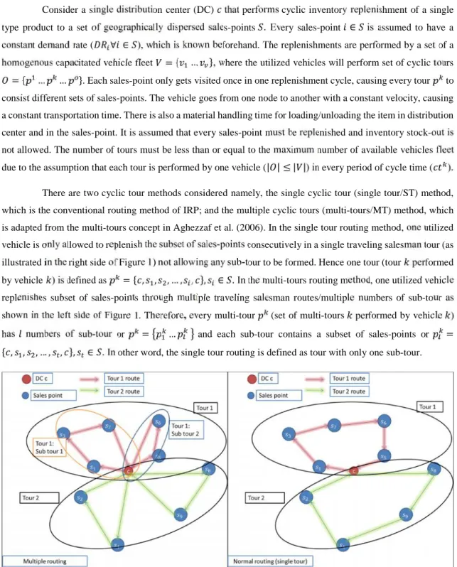
Consider a single distribution center (DC) that performs cyclic inventory replenishment of a single type product to a set of geographically dispersed sales-points . Every sales-point ∈ is assumed to have a constant demand rate ( ∀ ∈ ), which is known beforehand. The replenishments are performed by a set of a homogenous capacitated vehicle fleet = { … }, where the utilized vehicles will perform set of cyclic tours = { … … }. Each sales-point only gets visited once in one replenishment cycle, causing every tour to consist different sets of sales-points. The vehicle goes from one node to another with a constant velocity, causing a constant transportation time. There is also a material handling time for loading/unloading the item in distribution center and in the sales-point. It is assumed that every sales-point must be replenished and inventory stock-out is not allowed. The number of tours must be less than or equal to the maximum number of available vehicles fleet due to the assumption that each tour is performed by one vehicle (| | ≤ | |) in every period of cycle time ( ). There are two cyclic tour methods considered namely, the single cyclic tour (single tour/ST) method, which is the conventional routing method of IRP; and the multiple cyclic tours (multi-tours/MT) method, which is adapted from the multi-tours concept in Aghezzaf et al. (2006). In the single tour routing method, one utilized vehicle is only allowed to replenish the subset of sales-points consecutively in a single traveling salesman tour (as illustrated in the right side of Figure 1) not allowing any sub-tour to be formed. Hence one tour (tour performed by vehicle ) is defined as = { , , , … , , }, ∈ . In the multi-tours routing method, one utilized vehicle replenishes subset of sales-points through multiple traveling salesman routes/multiple numbers of sub-tour as shown in the left side of Figure 1. Therefore, every multi-tour (set of multi-tours performed by vehicle ) has numbers of sub-tour or = … and each sub-tour contains a subset of sales-points or = { , , , … , , }, ∈ . In other word, the single tour routing is defined as tour with only one sub-tour.
The following are the defined notation: Parameters
: Demand rate at sales-point (ton per hour)
: Distance between node to where , include DC and sales-point (kilometer) : Transportation time between node to where , include DC and sales-point (hour) : Material handling rate (ton per hour)
: Average speed of the utilized vehicle (kilometer per hour) : Maximum capacity of the utilized vehicle (ton)
: Capacity per warehouse in sales-point (ton/unit)
: Fuel efficiency rate of vehicle without any load (kilometer per liter) : Vehicle load to fuel consumption reduction rate (kilometer kilogram per liter) : Fix operational cost of the operating vehicle ($ per cycle)
: Transportation cost of the operating vehicle ($ per kilometer) : Fix handling cost in each sales-point ($ per cycle)
: Variable handling cost in each sales-point ($ per hour)
: Fix cost for utilizing per unit warehouse capacity in each sales-point ($ per KWh) : Variable holding cost in each sales-point ($ per unit hour)
: Total transportation cost ($ per hour) : Total material handling cost ($ per hour) : Total item storage cost ($ per hour)
: Energy consumed for utilizing unit of warehouse capacity (KWh/hour) : Emission produced for each liter of fuel used by vehicle (Kg eq.CO2 per liter) : Emission produced by performing material handling (Kg eq.CO2 per KWh) : Emission produced by carrying inventory (Kg eq.CO2 per KWh)
: Total transportation emission (Kg eq.CO2 per hour) : Total material handling emission (Kg eq.CO2 per hour) : Total inventory emission (Kg eq.CO2 per hour)
: Minimum cycle time for cyclic tour performed by vehicle (hour) : Maximum cycle time for cyclic tour performed by vehicle (hour) : Maximum cycle time for sub-tour in cyclic tour (hour)
: Cycle time for optimizing cost for cyclic tour (performed by vehicle ) (hour)
Decision variables
: Decision to go from node to node at sub-tour in tour : Decision to use vehicle
: Cycle time of multi-tours
: Level of item carried by vehicle when about to go from node to node ̅ : Average inventory level of the sales-point (ton)
: Material handling time in the sales-point (hour)
: Material handling time in the DC to initiate sub-tour in cyclic tour (hour) : Expected item to be delivered to sales-point (ton)
: Expected item to be carried on the sub-tour in cyclic tourv(ton) 3.2. Cycle time formulation
Cyclic tour performs repetitive inventory replenishments to every sales-point where the repetition between each successive cyclic tour (one cycle) is separated by a period of cycle time. It is assumed that the transportation time occurs in one cycle also consider the material handling duration where the material handling duration depends on the quantity of the item ordered in one sales-points.
Given the definition of cyclic tour = … , ∈ , every is bounded by the maximum and minimum tour’s cycle time.The definition of the maximum and minimum cycle time will become the upper and
lower bound of the cycle time. The maximum and minimum cycle time of the tour must be firstly defined to obtain the tour’s cycle time.As defined in the previous section, a single tour can be considered as a multi-tour with one sub-tour ( = { }), therefore making a same cycle time formulation for both cyclic tour methods.
Minimum cycle time is the minimum required time to perform one complete cyclic tour (cyclictour’s lower bound time), where it must be equal or larger than the time for one vehicle to finish the whole activities occurring in one cyclic tour as in (1). The right hand side of (1) consists of the occurred activities in , namely, the transportation time in tour , inventory replenishment handling time in every sales-point ( ) in tour where ∈ , and vehicle loading time in distribution center in every sub-tour of tour where ∈ . Equations (2) to (4) describe: the handling time for loading the item to vehicle in every sub-tour , the required item per sales-point in tour , and the total loaded item quantity to the vehicle in each sub-tour respectively.
= ⁄ + + ∈ = ⁄ ; ∀ ∈ = ; ∀ ∈ ; ∀ ∈ = ∈ ; ∀ ∈
The second and third component in the right-hand side of (1) can be substituted by (3) and (2). Since for every sub-tour equals to the summation of every in that sub-tour, they can be substituted into (5).
+ ∈
= ⁄ + ⁄
∈
= 2 ⁄
Thus, by substituting the handling time and loading time in (5) back into (1), the minimum cycle time for each tour is defined as in (6).
= ⁄ 1 − 2 ⁄
∈
Maximum cycle time is the upper bound of the tour’s cycle time which is related tothe vehicle’s maximum capacity. Therefore, every sub-tour in has their own maximum cycle time as in (7). The maximum cycle time in is defined as the shortest cycle time from the set of sub-tours’maximum cycle time as in (8).
=
∈ ∈
= min{ … }
3.3.
Objective function formulation
The objective functions defined in this cyclic IRP are the total cost rate per hour and total emission rate per hour. The formulation of both objectives function will be explained as follows.
3.3.1.
Cost rate formulation
The total cost rate in this model consists of three parts, namely, transportation cost, handling cost, and inventory holding cost. Transportation cost consists of fixed transportation cost per cycle and variable cost (distance cost) per cycle as in (9).
= ⁄ + ⁄
∈ ∈ ∈ ∈
The material handling activities include loading the item to the utilized vehicle in the distribution center for every sub-tour in every cyclic tour and unloading the item during the replenishment in each sales-point node. The material handling cost consists of fixed handling cost in each sales-point per cycle and variable handling cost (cost of consuming energy for performing material handling in both sales-points and DC) as in (10).
= ( / + / ) ∈ ∈ ∈ ∈ + ( / ) ∈ ∈ ∈
By using (3) and (2), the material handling cost in (10) can be substituted into (11):
= ( / + / ) ∈ ∈ ∈ ∈ + /( ) ∈ ∈ ∈
The inventory cost in (12) consists of fixed inventory cost for using numbers of thewarehouse’s capacity and average holding cost in one cycle time. Average inventory level in (13) is substituted to (12) resulting into (14). = ( ⌈ ⁄ ⌉ + ̅ ) ∈ ∈ ∈ ∈ ̅ = ⁄ ; ∀ ∈2 = ( . ⌈ ⁄ ⌉ + ⁄ )2 ∈ ∈ ∈ ∈
Thus, the total cost formulation is as in (15)
= + +
3.3.2.
Emission rate formulation
The total emission rate in this model comes from the vehicle fuel consumption, the energy consumed during material handling activity, and the energy used from the sales-point warehouse. The efficiency of the fuel consumption is influenced by the load factor in the vehicle as in (16) where the efficiency of the fuel consumption
gets worse as the vehicle’sload increase. The relation between vehicle weight to fuel consumption is defined using the formulated regression estimation in Coyle (2007).
= ⁄ − . . /
∈ ∈ ∈ ∈
During the material handling, the emission comes from the energy consumption when the item is unloaded from the vehicle and loaded into the vehicle as in (17).
= ( ⁄ ). . /
∈ ∈ ∈ ∈
The emission in the inventory holding activities come from the energy consumption in one cycle of the cyclic tour. The amount of energy used depends on the amount of warehouse capacity used as in (18).
= ⌈ ⁄ ⌉. . .
∈ ∈ ∈ ∈
The total emission formulation is as in (19).
= + +
3.4.
Multi-objective mix integer nonlinear model formulation
The objective functions are as in (20)min: ;min:
The constraints are as follows:
∈ ∈ ∈ = 1; ∀ , ∈ ≤ 1; ∀{ , , }, ∈ , ∈ , ∈ ≤ 1; ∀{ , , }, ∈ , ∈ , ∈ ∈ ∈ ∈ − ∈ ∈ ∈ = 0; ∀ ; ∈ S − = ∈ ; ∀ { , , }, { , } ∈ , ∈ ∈ ∈ ∈ − ∈ ∈ ∈ = ∈ ∈ ∈ ; ∀ ∈ ≤ ≤ ; ∀ ∈ ⁄ + ∈ ∈ ≤ ; ∀ { , }, ∈ , ∈ ≤ ; ∀ ∈ , ∈
= ∈
; ∀ { , }, ∈ , ∈ , ∈ {0,1}; ∀ { , , , }, { , } ∈ , ∈ , ∈
, ≥ 0; ∀ { , , }, { , } ∈ , ∈ , ∈
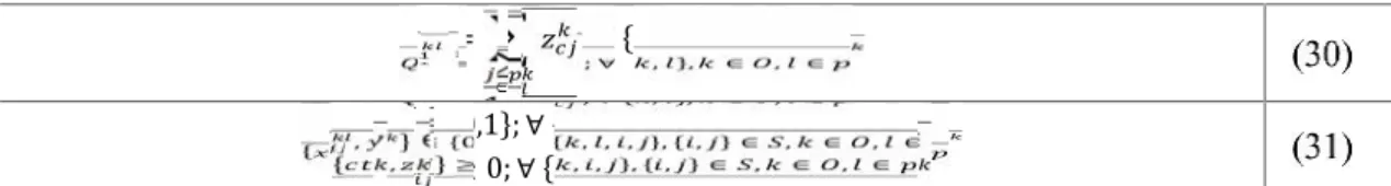
Constraint (21) to (23) ensure each node only visited once. Constraint (24) is a flow conservation constraint. Constraint (25) and (26) prevent the formation of sub sub-tour to happen. Constraint (27) and (28) define the upper and lower bound of the cycle time of each tour. Constraint (29) is vehicle capacity limitation. Constraint (30) defines the beginning of each sub-tour in each tour to have a sufficient amount of item to supply all node in one sub-tour route. Constraint (31) defines the decision variable type.
4.
Discrete multiple swarm PSO algorithm
Various metaheuristic methods are capable to yield a nearly optimal solution within limited times and resources. One of them is known as the particle swarm optimization (PSO), a swarm intelligence method algorithm that mimics bird flocks movement developed by Kennedy and Eberhart (1995). Many studies such as in The Jin Ai and Voratas Kachitvichyanukul (2009), T. J. Ai and V. Kachitvichyanukul (2009), Moghaddam et al. (2012), Mousavi et al. (2014)have shown the PSO’scapability to provide a high-quality solution in a routing problem type.
The proposed discrete multi-swarm PSO is developed by combining the discrete PSO concepts from Goldbarg et al. (2008) and Moghaddam et al. (2012) with the multi-swarms PSO concept from (Blackwell, 2007). Some PSO variants use multiple swarms (multi-swarms) to improve the PSO’s solution exploration capability and to reduce the chances of having premature convergence. It thus makes the multi-swarms PSO suitable for optimizing a problem with multiple peaks/optimal solution areas (Blackwell, 2007).
4.1.
Discrete multi-swarm PSO definition
Given a multiple of swarms where each of the swarm (sub-swarm) consists of agents/particles of solution that move inside a search space to perform solution searching. Each of theparticle’s movement gets influenced by the discrete velocity and solutions references.The particle’s velocityin this discrete PSO is defined as the probability value for a particle to be changed into one of the solution references, hence the movement of getting closer toward references solutions. The numbers of the solution references defined are the personal best (each particle’s personal best solution), local best (best solution in one swarm), global best (best solution among all swarm), arbitrarily best (taking the best particle from randomly selected particle inside the same sub-swarm). Among those references, there is also the probability of not getting changed into one of the solution references. The proportion of probability for choosing the solution reference will change along with the progression of the PSO’s iteration, therefore, affecting on how much the influence of solutions references to the particle’s movement. After updating the particle’s positionbased on the velocity value, each particle is tweaked by using heuristic algorithms (explained further in section 4.3). The description of the pseudo code of the proposed PSO algorithm is in Table 1.
Initialization of the parameter:(maximum iteration, swarm number,
particle number, inertia value (c1in,c2in,c3in , c1f, c2f, c3f), particle dimension personal best, local best, global best, valpar, valPbest, valLbest, valGbest)
for i=1 to maximum iteration
ci1=c1in-(c1in-c1f)*i/maximum iteration ci2=c2in-(c2in-c2f)*i/maximum iteration ci3=c3in-(c3in-c3f)*i/maximum iteration ci4=c4in-(c4in-c4f)*i/maximum iteration for j=1 to swarm number
for k=1 to particle number
valpar(j,k)=evaluate function for particle dimension(j,k)*
if valpar(j,k)< valPbest then
update value and dimension of personal best end if
if valpar(j,k)< valLbest then
update value and dimension of local best end if
if valpar(j,k)< valGbest then
update value and dimension of global best end if
proba =random number (0~1)
if proba < (ci1) then (the arbitrarily best)
random= randomly choose a set of number particle inside one swarm then pick one with the best value
particle dimension(j,k)= random elseif proba < (ci1+ci2) then (the personal best)
particle dimension(j,k)= personal best(j,k) elseif proba< (ci1+ci2+ci3) then (the local best)
particle dimension(j,k)= local best(k) else (the global best)
particle dimension(j,k)= global best end if
if (random number (0~1))< threshold** (local optimization)
1/3 chances to choose tour formation using either heuristic method 1; method 2, or method 3
else
tour formation using heuristic method 4 end if
next k next j
next i
save the global best value and global best dimension
* (consisted of constructing the tour and vehicle assignment, solution feasibility checking, minimizing the assigned objective function) ** the value of threshold is adjustable, default: 0.5
4.2.
Decoding PSO
’s
discrete dimension to configure the cyclic tour
The discrete dimension is an array of integer numbers that are used inside the PSO by decoding them into a set of cyclic tours. The information inside the particle defines the routing decision variables ( and ). The others decision variables are determined after defining the routing decision variables (explained further in section 4.4). The particle decodingis used to evaluate each particle’s solution quality (inTable 1).
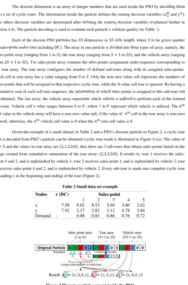
Each of the discrete PSO particles has3 dimensions or3 cells length, where is the given number of sales-point nodes (not including DC). The array in one particle is divided into three types of array, namely, the sales-point array (ranging from1to ), the tour array (ranging from + 1to2 ), and the vehicle array (ranging from2 + 1to3 ). The sales-point array contains the sales-points assignment order/sequence corresponding to the tour array. The tour array configures the number of defined sub-tours along with its assigned sales-points. Each cell in tour array has a value ranging from 0 to . Only the non-zero value cell represents the numbers of sales-points that will be assigned to that respective cyclic tour, while the0value cell tour is ignored. By having a cumulative sum of each cell tour sequence, the information of which sales-points is assigned to this sub-tour can be obtained. The last array, the vehicle array represents which vehicle is utilized to perform each of the formed sub-tour. Vehicle cell’s value ranges between 0 to , where 1 to represent which vehicle is utilized. The cell value in the vehicle array will have a non-zero value only if the value of cell in the tour array is non-zero as well, otherwise, the vehicle cell value is 0 when the tour cell value is 0.
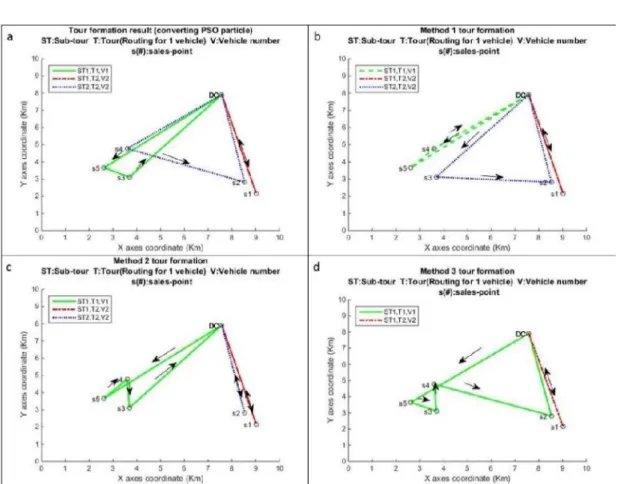
Given the example of a small dataset in Table 2 and aPSO’sdiscrete particle in Figure 2, a cyclic tour that is decoded from PSO’s particle can be obtained (cyclic tour result is illustrated inFigure 4 (a)). The value of S = 5and the values in tour array are(2,1,2,0,0), thus there are 3 sub-tours that obtain sales-points based on the range created from cumulative summation of the tour array:(2,3,5,0,0). It results in: tour 1 receives the sales-point 5 and 3, and is replenished by vehicle 1; tour 2 receives sales-sales-point 1, and is replenished by vehicle 2; tour 3 receives sales-point 4 and 2, and is replenished by vehicle 2. Every sub-tour is made into complete cyclic tour by addingcin the beginning and ending of the tour (Figure 2).
Table 2 Small data set example
Nodes
r (DC)
Sales-point
1
2
3
4
5
x
7.58
9.02
8.53
3.69
3.60
2.62
y
7.92
2.17
2.82
3.12
4.78
3.66
Demand
-
0.08
0.83
0.86
0.76
0.72
4.3.
Heuristic method for tweaking the particle of the PSO
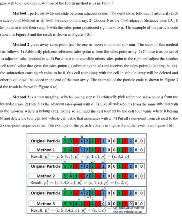
This study proposes four heuristic methods to perform local optimization to the solution carried by each particle (referring to the local optimization part in pseudocode Table 1) which are followed by examples to tweak the particle in Figure 2. The conversion of the particle from the first three heuristic methods is as in Figure 3 and Figure 4 (b to c) and the illustration of the fourth method is as in Table 3.
Method 1 performs swap and slide between adjacent nodes. The steps are as follows: 1) arbitrarily pick one sales-point (defined as ) from the sales-point array. 2) Choose as the most adjacent (distance wise ( )) sales-point to and then swap with the sales-point positioned right next to . The example of the particle code is shown in Figure 3 and the result is shown in Figure 4 (b).
Method 2 gives away sales-point (can be one or more) to another sub-tour. The steps of this method are as follows: 1) Arbitrarily pick one reference sales-point from the sales-point array. 2) Choose as the set of most adjacent sales-point(s) to . 3) Put next to and slide others sales-point to the right and adjust the number of cell tours’ value that gives the sales-point(s) (subtracting the ) and receives the sales-point(s) (adding the ). If the subtraction causing value to be 0, this cell tour along with the cell in vehicle array will be deleted and another 0 value will be added in the end of the tour array. The example of the particle code is shown in Figure 3 and the result is shown in Figure 4 (c).
Method 3 is a tour merging, with following steps: 1) arbitrarily pick reference sales-point from the sales-point array. 2) Pick as the adjacent sales-point with . 3) Give all sales-points from the same sub-tour with to the sub-tour where belong ( ). Doing so will add the cell tour by the cell tour value where belong ( ) and delete the tour cell and vehicle cell value that associates with . 4) Put all sales-point from next to the last sales-point sequence in . The example of the particle code is in Figure 3 and the result is in Figure 4 (d).
Method 4, the random swapping order method is a particle modification that randomly swaps the order of the information in the array. Random swap method changes the sequence of one array making every array has a swapping chance of 1/3 when this method is selected. The steps are as follows: 1) choose randomly from one of the three arrays. 2) arbitrarily choose 2 cells with non-zero values from the randomly selected array from step 1. 3) There are four possibilities (25% of each) for sequence changing similar with the mutation principle in GA, namely, keep the original sequence, swap between the two cells, slide the sequence between two cells and flip sequence between two cells. The given example in Table 3 shows the order swapping in the sales-point array.
Table 3 Method 4 Result Example for sales-point array
Method Sales-point array
dimension
Original sequence (do nothing) 5 3 4 1 2
Swap (swam 3 and 2) 5 2 4 1 3
Flip (flip sequence from 3 to 2) 5 2 1 4 3
Slide (put 3 next to 2) 5 4 1 2 3
seq1 (arbitrary cell 1): 3 seq2 (arbitrary cell 2): 2
Note: seq1 always precede seq2 sequence’s
Figure 4 (a) Tour formation result from the PSO particle; (b) Method 1 tour formation result example; (c) Method 2 tour formation result example; (d) Method 3 tour formation result example
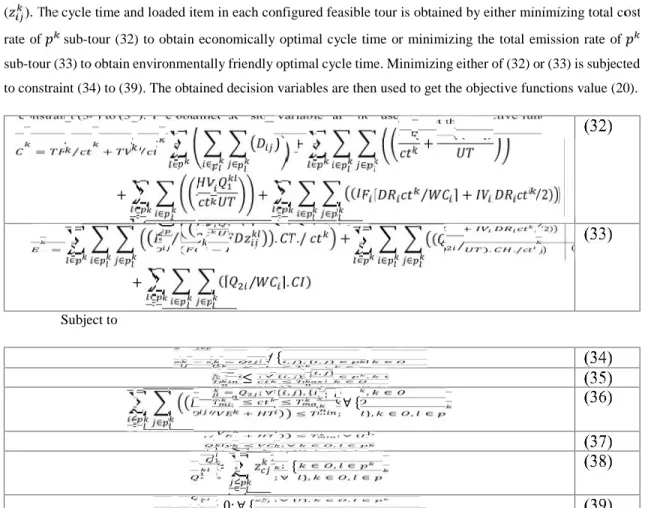
Due to the non-linear formulation of the objectives function, the cyclic tour is configured by decoding the discrete dimension in each particle into two steps. The first step is related with configuring the cyclic tour routing decision ( and ) which has been mentioned in section 4.2. Before continuing to the next step, the feasibility of the configured cyclic tour will be evaluated. If the solution by this particle is infeasible, it will be penalized by a large value. If the configured route is feasible (not violating constraint (21) to (24), (27) and (28)), the minimum and maximum cycle time in each tour will be determined (as in section 3.2) and then it is followed by determining the decision related with the replenishment policy, namely, the cycle time ( ) and loaded item ( ). The cycle time and loaded item in each configured feasible tour is obtained by either minimizing total cost rate of sub-tour (32) to obtain economically optimal cycle time or minimizing the total emission rate of sub-tour (33) to obtain environmentally friendly optimal cycle time. Minimizing either of (32) or (33) is subjected to constraint (34) to (39). The obtained decision variables are then used to get the objective functions value (20).
= ⁄ + ⁄ ∈ ∈ ∈ + + ( ) ∈ ∈ ∈ + ∈ ∈ + ( ⌈ ⁄ ⌉ + ⁄ )2 ∈ ∈ ∈ = ⁄ − . ./ ∈ ∈ ∈ + ( ⁄ ). ./ ∈ ∈ ∈ + (⌈ ⁄ ⌉. ) ∈ ∈ ∈ Subject to − = ; ∀ { , }, { , } ∈ , ∈ ≤ ≤ ; ∈ ⁄ + ∈ ∈ ≤ ; ∀ { }, ∈ , ∈ ≤ ; ∀ ∈ , ∈ = ∈ ; ∀ { }, ∈ , ∈ , ≥ 0; ∀ { , , }, { , } ∈ , ∈ , ∈
4.5.
Discrete multi-swarms PSO performance comparison confirmation
In this section, the discrete swarms PSO is used to replicate the numerical example of cyclic multi-tours IRP by Aghezzaf et al. (2006). The discrete multi-swarms PSO’s solution in this study is compared with the column generation method’s solution used in their formulated cyclic multi-tours IRP problem. Due to the structural similarities of IRP problem between the MOCGIRP and their formulated cyclic multi-tours IRP, this comparison could give an approximation of the proposed PSO’sperformance. The parameter used in the PSO is as shown in Table 4 (this parameter setting also used in the later numerical example section).
Table 4 Set of Parameter Used in PSO
General information Inertia value Initial (cin) Final (cf)
Particle number (per swarm) 50 Inertia 2 (personal best 0.15 0.15
Sub-swarm (number of swarms) 18 Inertia 3 (local best) 0.04 0.15
Discrete dimension 3 Inertia 4 (global best) 0.01 0.3
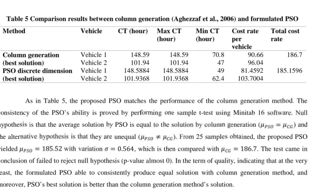
Table 5 Comparison results between column generation (Aghezzaf et al., 2006) and formulated PSO
Method Vehicle CT (hour) Max CT
(hour) Min CT (hour) Cost rate per vehicle Total cost rate Column generation (best solution) Vehicle 1 148.59 148.59 70.8 90.66 186.7 Vehicle 2 101.94 101.94 47 96.04
PSO discrete dimension (best solution)
Vehicle 1 148.5884 148.5884 49 81.4592 185.1596
Vehicle 2 101.9368 101.9368 62.4 103.7004
As in Table 5, the proposed PSO matches the performance of the column generation method. The consistency of the PSO’s ability is proved by performing one sample t-test using Minitab 16 software. Null hypothesis is that the average solution by PSO is equal to the solution by column generation ( = ) and the alternative hypothesis is that they are unequal ( ≠ ). From 25 samples obtained, the proposed PSO yielded = 185.52with variation = 0.564, which is then compared with = 186.7. The test came in conclusion of failed to reject null hypothesis (p-value almost 0). In the term of quality, indicating that at the very least, the formulated PSO able to consistently produce equal solution with column generation method, and moreover, PSO’s best solution is better than the column generation method’s solution.
4.6.
Normalized normal constraint method to solve multi-objective problem
This study presents the solution as a set of multiple non-dominated solutions or referred as Pareto optimal solution. The Pareto optimal solution/Pareto set consists of a set of Pareto points (consisting of multi-objectives solutions) with values that gradually shift from optimizing one objective function into other ones. This set of solution can be obtained by using the aggregate objective function (AOF) to solve the numbers of aggregated objective with varyingobjective function’sscale and weighting (Wang et al., 2011). However, finding a good scale and weighting for each objective function are the crucial deciding factors to a produce a well-balanced Pareto set that can facilitate a managerial insight. Therefore, to avoid objective function scaling deficiencies, this paper adopts the normalized normal constraint method for bi-objective case principle which explained thoroughly in section 3.1 of Messac et al. (2003). Following is the description of the normalized normal constraint method.
Performing normalized normal constraint method requires the set of anchor points (step 1: obtaining the anchor point), denoted by ∗= { ( ∗), ( ∗)}and ∗= { ( ∗), ( ∗)}, where each of anchor point is the best solution for each objective function respectively. The line between the anchor points is called as the utopia line that gives direction in Pareto points generation in the later step. The next step is the objective function values normalization (step 2: objectives mapping). The scale/length of each objective function could be defined as = ( ∗) − ( ∗)and = ( ∗) − ( ∗)respectively. These scales will be used to yield a normalized objective function value = [ ( ), ( )] into ̅ = ( ) − ( ∗) / , ( ) − ( ∗) / . The next step is to decide the direction of obtaining the Pareto points in the Pareto set (step 3: Utopia line vector) by following the vector = ̅ ∗− ̅ ∗= [1, −1]that is used to change the weighting value of each objective function. The next step (step 4: normalized increments) is to determine the value of an increment in coefficient
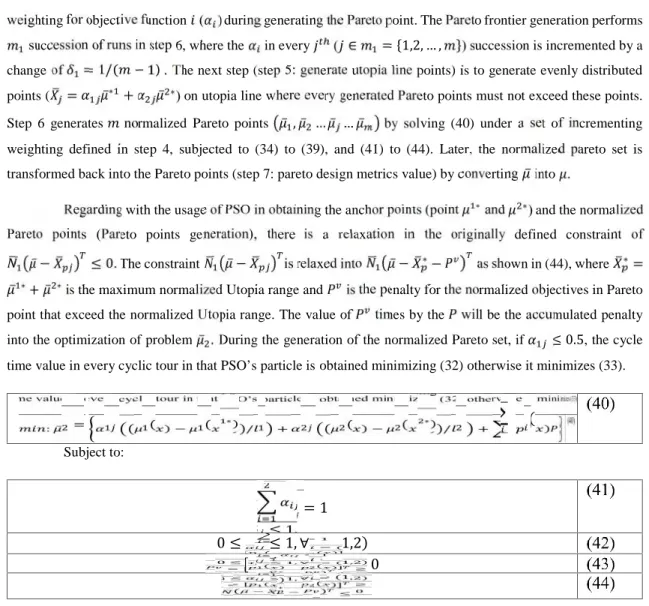
weighting for objective function ( ) during generating the Pareto point. The Pareto frontier generation performs succession of runs in step 6, where the in every ( ∈ = {1,2, … , }) succession is incremented by a change of = 1/( − 1). The next step (step 5: generate utopia line points) is to generate evenly distributed points ( = ̅∗ + ̅ ∗) on utopia line where every generated Pareto points must not exceed these points. Step 6 generates normalized Pareto points ̅ , ̅ … ̅ … ̅ by solving (40) under a set of incrementing weighting defined in step 4, subjected to (34) to (39), and (41) to (44). Later, the normalized pareto set is transformed back into the Pareto points (step 7: pareto design metrics value) by converting ̅into .
Regarding with the usage of PSO in obtaining the anchor points (point ∗and ∗) and the normalized Pareto points (Pareto points generation), there is a relaxation in the originally defined constraint of ̅ − ≤ 0. The constraint ̅ − is relaxed into ̅ − ∗− as shown in (44), where ∗= ̅ ∗+ ̅ ∗is the maximum normalized Utopia range and is the penalty for the normalized objectives in Pareto point that exceed the normalized Utopia range. The value of times by the will be the accumulated penalty into the optimization of problem ̅ . During the generation of the normalized Pareto set, if ≤ 0.5, the cycle time value in every cyclic tour in that PSO’s particle isobtained minimizing (32) otherwise it minimizes (33).
: ̅ =
( ) − (
∗) /
+
( ) − (
∗) /
+
( )
Subject to:= 1
0 ≤
≤ 1, ∀ = (1,2)
= [ ( )
( )] ≥ 0
̅ −
∗−
≤ 0
5.
Computational results
The MOCGIRP model along with the solving method are all built in the MATLAB R2014b environment which will be used to solve the numerical example. The analyses of the numerical example are explained in the following. Sub-section 5.1 analyzes the Pareto set of the cyclic single tour (ST) method. Sub-section 5.2 compares and analyzes the Pareto set of the cyclic multi-tours (MT) and the ST method. Sub-section 5.3 performs sensitivity analyses of several parameters on both ST and MT method. The parameters used in this section are given in Table 6 and Table 7.
Table 6 Parameter Set (default parameter setting) Nodes : 15
Vehicle : 6 (identical vehicle) : 44 ton per hour : 50 Km per hour : 44 ton
: 30 ton
: 9.701 Km per liter : 0.165 Km per liter
: 50 $ per cycle : 1 $ per kilometer : 50 $ per hour : 1 $ per hour : 0.1 $ per unit
: 0.22 $ per hour (conEdison, 2015; MGOE, 2015) : 2.61 Kg per liter fuel (Ubeda et al., 2011) : 14.82 Kg per hour
: 1 Kg eq.CO2 per kWh
: 1.21 KWh per hour (Li et al., 2012)
Table 7 Distance and demand rate parameter Node Node coordinates
(km)* (ton/hour)
Node Node coordinates (km)*
DR (ton/hour)
x-axis y-axis x-axis y-axis
400.11 350.15 - 8 663.72 168.02 0.97 1 918.79 129.41 0.17 9 41.91 406.48 0.19 2 495.21 431.00 0.22 10 203.65 432.58 0.59 3 54.02 126.26 0.08 11 693.85 3.74 0.92 4 637.89 735.61 0.28 12 676.72 750.98 0.74 5 640.22 453.88 0.93 13 545.37 167.14 0.92 6 462.66 837.28 0.48 14 752.01 533.98 0.36 7 391.17 710.45 0.55 15 123.64 251.78 0.95
* obtained by calculating Euclidian distance between each node coordinates
5.1.
Tradeoff in the cyclical IRP Pareto set
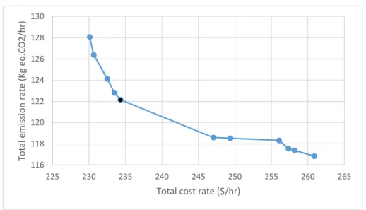
The analyses of the tradeoff between the two objectives function in this sub-section are using the ST method Pareto frontier set (as in Figure 5). The Pareto set is formed between the anchor points which consist a solution that minimizes the total cost rate (TC-opt) and the solution that minimizes total emission rate reduction (TE-opt). The cost and emission rate breakdown for TC-opt and TE-opt in Table 9 show that both inventory holding and material handling activities still have considerable value toward cost and emission rate, even though not as significant as the transportation activities. Those two logistics operations yield 18.59% of the total cost and 26.19% of the total emission for the TC-opt solution; and 16.62% of the total cost and 23.77% of the total emission rate for the TE-opt solution. This result shows the idea that integration of inventory holding and material handling with the transportation activities are omitted could bring considerable loss of information to the decision-making, which highlights their importance in the IRP formulation.
Figure 5 Pareto Frontier Solution of Dispatching Vehicle in Single Tour Method
Table 8 Set of Pareto frontier solution in dispatching vehicle in single tour method Total cost rate ($/hr) Total emission rate (kg eq. CO2/hr) Avg. loaded per vehicle (ton) Avg. replenishment/sales-points (ton) Normalized value * 230.10 128.07 44.00 17.60 1 230.64 126.39 44.00 17.60 0.87 232.51 124.13 44.00 17.60 0.73 233.48 122.82 43.52 17.41 0.64 *** 234.31 122.15 43.47 17.39 0.61 247.04 118.59 41.10 16.44 0.71 249.38 118.52 40.56 16.22 0.78 256.04 118.32 39.25 15.70 0.97 257.33 117.56 38.69 15.47 0.95 258.14 117.38 38.54 15.42 0.96 ** 260.87 116.84 38.12 15.25 1
* TC-opt; ** TE-opt; *** best practice solution
Figure 5 and Table 8 show the tradeoff between the two objective functions while the detailed comparison between TC and TE-opt solution is in Table 9 and Table 10. In the TC-opt solution, the vendor maximizes vehicles load capacity and seeks the shortest route to reduce the frequency of replenishment, reducing the transportation cost. A Higher quantity of the item is loaded in the sales-points, indicating an increase in the number of warehouse capacity utilized due to the usage of larger capacity of inventory. Overall, the comparison between TC-opt and TE-opt method shows that the reduction in the variable transportation cost outweighs the increase from the other costs resulting in the total cost rate reduction. However, optimization of the total cost rate leads to worse vehicle fuel and warehouse energy consumption, hence the high emission rate.
In contrast, the TE-opt solution yields a routing configuration to minimize the emission by minimizing the average load per vehicle and the quantity replenishment in every sales-point. These result in less fuel consumption and warehouse energy consumption (less unit of warehouse utilized), hence explaining the emission reduction. But this TE-opt configuration, however, raises the operational cost as well due to the shorter cycle time, thereby increasing the total cost rate.
116 118 120 122 124 126 128 130 225 230 235 240 245 250 255 260 265 To ta l e m iss io n ra te (K g eq .C O2/h r)
Figure 5 (the Pareto points with black dot) and Table 8 (solution with *** mark) also show the Pareto point with the smallest normalized aggregated objectives function value. This Pareto point provides a well-balanced cost and emission rate minimization for the best practice solution reference. With this in mind, the TC-opt, TE-TC-opt, and smallest normalized Pareto point could offer insight into managerial decision making.
5.2.
Comparison between cyclic single tour and cyclic multi-tours method
This section compares ST and MT method under the situation of six units of vehicle available where the detail of comparison is shown in the dataset of ST6 and MT6 in Figure 6 and in Table 9.
One MT routing method consists numbers of sub-tours, causing longer total distance to complete than the ST. The higher capacity of replenishment and longer distance to complete one tour lead to the longer and broader cycle time range thus, increasing the tradeoff between TC-opt and TE-opt solution. Table 10 gives detail comparison and confirmation that the MT method has longer and more varied cycle times, higher average replenishment per sales-point than the ST method. However, since MT method breaks down the replenishment of sales-points of an assigned vehicle into numbers of smaller sub-tours, more flexibility is expected in utilizing vehicle’s limited capacity to replenish each sales-point than the ST method. As a result, MT method can produce a significantly superior Pareto set than the ST method. Total cost reduction is reached by longer cycle time that reduces the replenishment frequencies. While total emission reduction is achieved by dispatching vehicle as light as possible and utilizing the smallest unit of the warehouse while keeping the inventory in sales-point enough for going through minimal cycle time. To put it in comparison, the TC-opt solution of the MT method yields 17.85% lower total cost rate and 3.68% lower total emission rate than the ST method, while the TE-opt solution yields 11.95% lower total cost rate and 7.72% lower total emission rate than the ST method.
Table 9 Performance comparison between single tour, multi-tours under 6 vehicle fleet available Single tour method Multi-tours method
TC-opt TE-opt TC-opt TE-opt
C o st r a te
Transportation fixed cost 9.48 10.90 4.76 6.88
Transportation variable cost 177.85 206.62 138.70 182.49
Handling fixed cost 24.66 27.54 11.60 17.11
Handling variable cost 0.38 0.38 0.38 0.38
Inventory holding cost 13.20 11.44 26.65 18.32
Inventory fixed cost 4.53 3.99 6.92 4.53
Total Cost rate 230.10 260.87 189.01 229.71
E mi ss io n ra te Transportation emission 101.88 93.06 86.28 81.63 Inventory emission 20.57 18.15 31.46 20.57 Handling emission 5.62 5.62 5.62 5.62
Total emission rate 128.07 116.84 123.36 107.82
* Cost rate is in $/hour; Emission rate is in Kg eq.CO2/hour
Table 10 Comparison of result between single tour, multi-tours under 6 vehicle fleet available Single tour
method
Multi-tours method TC-opt TE-opt TC-opt TE-opt
Number of vehicle (unit) 6 6 6 6
Capacity (ton) 44 44 44 44
Cycle time average (hour) 33.52 28.69 88.01 59.67
Longest cycle time (hour) 42.84 35.58 226.80 150.04
Average vehicle load per tour (sub-tour in cyclic
multi-tours) (ton) 44.00 38.12 41.00 33.32
Average replenishment per sales-point (ton) 17.60 15.25 35.53 24.43 Total distance covered per cycle (Km) 5693.96 5838.70 9712.83 8518.15
Figure 6 Comparison between single tour, multi-tours under different vehicle fleet available (Note: The ST 5 data set is not displayed in the figures because of this parameter setting yielded infeasible solution)
5.3.
Sensitivity analyses
This section explores how the changes in parameter value affect the total cost rate, total emission rate, and the tradeoff relationship in both ST and MT method. Therefore, sensitivity analyses are performed toward several parameters, namely, vehicle fleet number, inventory capacity, vehicle load capacity, inventory energy consumption and vehicle fuel consumption. The Pareto datasetwith ‘default’ name is using the parameter setting in Table 6 and is used as the comparison toward the changed parameter Pareto set result.
5.3.1.
Change in the available vehicle fleet number
Here, Figure 6 shows the comparison of the Pareto set between of different vehicle numbers, namely, 5, 6 (the default value), and 7 vehicles for both ST and MT method. For the ST method, larger fleet number increase the total vehicle capacity for replenishment thereby improving the maximum item loaded and the economics of scale. It resulted in the reduction of both total cost rate and total emission rate. This is shown by the ST7 Pareto set being the superior set than the ST6 Pareto set in both cost and emission rate, even though it is not as better as the cyclic MT method in Figure 6. On the other hand, ST method cannot yield feasible solution under the setting of 5 available vehicle fleet as the result of the insufficient capacity to replenish the whole sales-point.
When the vehicle dispatched using the MT method, the change in the number of vehicle fleet does not affect the Pareto set as significant as the ST Pareto set. This is shown by the Pareto sets of MT method under the different number of available vehicles are overlapping with each other. However, this parameter also shows the
105 110 115 120 125 130 180 190 200 210 220 230 240 250 260 270 To ta l e m iss io n ra te (K g eq .C O2/h r)
Total cost rate ($/hr)
MT capability to replenish the whole sales-point using 5 vehicles when the ST method yield the infeasible solutions, therefore proving its higher degree of flexibility than the ST method.
5.3.2.
Change in sales-point inventory capacity and vehicle capacity
A similar pattern happened between the Pareto set of ST and MT method when the vehicle capacity (Figure 7) and inventory capacity parameter (Figure 8) are changed. The results of vehicle capacity sensitivity analysis show that higher vehicle capacity (48 ton) enables the vehicle to load more item with consequences of higher energy consumption, thereby causing higher emission rate on optimizing total cost and enlarging the tradeoff range of the Pareto set than the normal vehicle capacity (40 ton). In contrast, lower vehicle capacity (40 ton) reduces the item load capability, forcing more frequent replenishment but utilizes less energy. As a result, it causes lower emission rate in optimizing total cost and reduces the tradeoff range of the Pareto set from the normal vehicle capacity.
The results of inventory capacity parameter sensitivity analysis show that the larger sales-point inventory capacity (1.1 times of default sales-point inventory capacity) allows the adjacent Pareto points to the TC-opt having lower emission rate as the result of the lower energy usage ratio (inventory capacity to energy consumption per unit inventory ratio). The opposite effect happens on the smaller sales-point inventory capacity (0.9 times of the default value) because of the adjacent Pareto points to the TE-opt solution have higher emission rate due to the higher energy consumption. However, the change in capacity value’s effect is morenoticeable in the MT Pareto sets than in the ST Pareto set, where the Pareto sets of ST are more overlapping with each other.
Figure 7 Comparison of various vehicle capacity for single tour routing and multi-tours routing 105 110 115 120 125 130 135 140 145 175 185 195 205 215 225 235 245 255 265 To ta l e m iss io n ra te (K g eq .C O2/h r)
Total cost rate ($/hr)
Figure 8 Comparison of various inventory capacity for single tour routing and multi-tours routing
5.3.3.
Change in inventory energy consumption and vehicle fuel consumption
The vehicle fuel efficiency in Figure 9 and inventory energy consumption in Figure 10 affect the Pareto set in a similar pattern for both MT and ST method. Change in vehicle fuel efficiency gives a significant effect toward the tradeoff on the Pareto set. Higher fuel efficiency (1.1 times of the normal fuel efficiency value) makes less carbon emission production and reduces vehicle load effect toward the fuel consumption. As a result, it shifts the Pareto set to the lower emission rate level than the default Pareto set and reduces cost and emission rate’s tradeoff range. The opposite thing happens for worse fuel efficiency (0.9 times of the normal fuel efficiency value), amplifying the effect of heavier weight causing worse fuel efficiency, then further resulting in higher emission rate. As a result, it creates broader tradeoff range between TC-opt and TE-opt solution and worse Pareto set value than the default ST Pareto set.
Energy consumption in the sales-point inventory gives similar but more significant effect toward the Pareto set than the sales-point inventory capacity parameter in Figure 8. The higher sales-points inventory energy consumption (1.1 times of the default inventory energy) shifts the whole Pareto set vertically up from the default Pareto set for both ST and MT Pareto set due to the higher emission rate. The opposite effect happens on lower sale-points inventory energy consumption (0.9 times of the default inventory energy), where the Pareto set shifts vertically down from the default Pareto set for both ST and MT Pareto set.
100 105 110 115 120 125 130 185 195 205 215 225 235 245 255 265 To ta l e m iss io n ra te (K g eq .C O2/h r)
Total cost rate ($/hr)
Figure 9 Comparison of various fuel efficiency for single tour routing and multi-tours routing
Figure 10 Comparison of various inventory energy usage rate for single tour routing and multi-tours routing
6.
Conclusion
This study addresses the issues of green logistics management by proposing the MOGCIRP model. Activities defined inside the MOGCIRP are the transportation, material handling, and inventory holding activity, which are the majority activities inside the logistics management. Realistic conditions, namely, material handling time, a vehicle with a load-dependent fuel consumption, and the hourly cycle time are considered inside the cyclic IRP formulation to represent a realistic and accurate green logistics operation.
90 100 110 120 130 140 150 160 170 180 180 200 220 240 260 280 To ta l e m iss io n ra te (K g eq .C O2/h r)
Total cost rate ($/hr)
ST Default ST Fuel0.9 ST Fuel1.1 MT Default MT Fuel 1.1 MT Fuel 0.9
100 105 110 115 120 125 130 135 185 195 205 215 225 235 245 255 265 To ta l e m iss io n ra te (K g eq .C O2/h r)
Total cost rate ($/hr)
The solution for the MOCGIRP is provided as a set of solutions (Pareto points) which is called as a Pareto frontier that is formed using the normalized normal constraint method. To solve the MOCGIRP to yield set of the solutions, this study proposes a discrete multi-swarm PSO along with the heuristic algorithms to perform local optimization for the PSO. The formulated PSO is tested by solving the numerical example of the cyclic IRP problem in Aghezzaf et al. (2006) and it is proven to be able to yield a high-quality solution.
The computational results show that transportation activities still have the biggest contribution to the total cost and emission rate (around 80% of both cost and emission). However, inventory holding and material handling activities also contribute the considerable value of cost and emission (around 20% of the total cost and emission rate). This result, therefore, emphasizes the importance of integrating and linking the transportation and inventory management activities in the green logistics management issues to provide an accurate result. There is also a tradeoff between optimizing cost rate and emission rate. Total cost rate optimization solution increases the fuel consumption, warehouse energy consumption due to more item stored, which leads to the increase in emission rate, while the opposite thing happened for emission rate optimization. Emission reduction is achieved by making more frequent replenishment and less energy usage in a consequence of higher cost.
The MT method gives more flexible capacity utilization to its fleet compared to ST method which results in the superior or dominating solution in both cost rate and emission rate compared to ST method. In average (averaging the TC-opt and TE-opt solution) MT method yields 40% lower total cost rate and 6.5% lower total emission rate compared with ST method.
The Pareto set gives an insight of the tradeoff happened between these two objectives and showing the well-balanced solution as well. Therefore, developing a method to find the best practices solution can be useful for decision maker (managerial implication). Also, from several parameters highlighted in sensitivity analyses sub-sections, some of the parameters give a significant effect towards the Pareto set and affect the tradeoff of the ST and MT cyclic IRP. It pinpoints the parameters that should be tuned to develop a greener vehicle, green source of energy in having a green logistics operation and yield a better economy as well.
6.1.
Suggestion and further research
As mentioned before, that not so many studies about IRP-related with green issues have been done. Some suggestions in the future such as 1) Formulating the model for the different condition of IRP (e.g. cold chain, multiple commodities, heterogenous fleet, etc.); 2) Considering sustainable factor such as energy cost, carbon trading to make a realistic model in the IRP; 3) Developed the IRP model by incorporating method such as backhauling (Pradenas et al., 2013; Ubeda et al., 2011), different modes of transport or utilizing friendly environmental vehicle(Ćirović et al., 2014; Erdogan & Miller-Hooks, 2012).