Article
Physics Parameterization Selection in RCM and ESM
Simulations Revisited: New Supporting Approach
Based on Empirical Copulas
Patrick Laux1,2,* , Noah Kerandi3and Harald Kunstmann1,2
1 Institute of Meteorology and Climate Research (IMK-IFU), Campus Alpine, Karlsruhe Institute of Technology (KIT), 82467 Garmisch-Partenkirchen, Germany; [email protected]
2 Institute of Geography, University of Augsburg, 86159 Augsburg, Germany
3 Institute of Mineral Processing and Mining, South Eastern Kenya University, P.O. Box 170-90200 Kitui, Kenya; [email protected]
* Correspondence: [email protected]; Tel.: +49-8821-183259
Received: 21 February 2019; Accepted: 12 March 2019; Published: 19 March 2019
Abstract: This study aims at a new supplementary approach to identify optimal configurations of physics parameterizations in regional climate models (RCMs) and earth system models (ESMs). Traditional approaches separately evaluate variable performance, which may lead to an inappropriate selection of physics parameterization combinations. Besides traditional approaches, we suggest an additional selection approach by considering the joint dependence structure (covariance structure) between key meteorological variables, i.e., precipitationPand temperatureT. This is accomplished by empirical P and T copula functions and the χ2-test, and is demonstrated in two locations
in Kenya with different major precipitation processes. It is shown that the selection based on traditional approaches alone may lead to nonoptimal decisions in terms of joint dependence structure betweenPandT. It was found that the copula-based approach may reduce the need for complex multivariate bias correction, as demonstrated using local intensity scaling forPand linear scaling for T. The new approach may contribute to improving RCM and ESM simulations and climate-impact studies worldwide.
Keywords:physics parameterization; regional climate models; earth system models; performance evaluation; empirical copula;χ2-test; bias correction
1. Introduction
The fidelity of regional climate models (RCMs) and earth system models (ESMs) in reproducing the observed regional climate provides confidence for the generation of regional climate projections for the future. RCMs and ESMs are still the tools of choice to derive future climate projections for climate-change-impact studies, such as in hydrology and agriculture (e.g., Reference [1]). In these disciplines, precipitationPand temperatureT(PandT) belong to the most important meteorological variables (e.g., References [2,3]) used for validation.
Recently, it was found that extreme precipitation markedly rises at higher atmospheric temperatures, faster than the rate of the atmosphere’s water-holding capacity (Clausius–Clapeyron equation). As a consequence of temperature increases induced by climate change, intensification of (extreme) precipitation intensities with regionally varying magnitudes is expected [4].
Similarly to the atmosphere, such a link betweenPandTalso exists for the lower atmosphere, next to Earth’s surface (e.g., Reference [5]). From this, it becomes obvious that a correct representation of the joint distribution of surfacePandTis a critical aspect for generating reliable RCM and ESM projections.
Atmosphere2019,10, 150 2 of 14
Even though their horizontal resolution is high (typically ranging in the order from 50 to 5 km), RCMs need to represent processes at smaller scales than those they can explicitly resolve. Besides land-surface processes, the most crucial processes to be parameterized in RCMs include radiation, convection, and cloud microphysics, partly with complex interactions. Oettli et al. [1], for instance, found that obtained results from two different physics configurations of the same RCM may be more distinct than the two different RCMs themselves. One of the key challenges is precipitation modeling: in an RCM, its generation is subdivided into a large-scale scheme, accounting for clouds and precipitation that result from atmospheric processes resolved by the models (e.g., cyclones and frontal systems), and a convection scheme, describing clouds and precipitation resulting from subgrid scale-convective processes [3]. Precipitation generation thereby involves many coupled processes between cumulus convection, cloud microphysics, radiation, land and ocean surface, and the planetary boundary layer [6].
The choice of the parameterization schemes has significant impact on climate projections (e.g., Reference [7]). It is therefore indispensable to identify a suitable physics parameterization combination prior to conducting a long-term RCM simulation (e.g., Reference [8]), but also short-term weather forecasts. Both for a full-factorial (e.g., References [9–11]) and a one-change-at-a-time approach (e.g., References [12–14]), analyses of the performance of different physical-parameter configurations are based on specific metrics, separately evaluated for the climate variables of interest. This is a severe limitation because it might lead to inappropriate selection of a configuration in terms of joint distributions of major variables, which may finally lead to complex and nonlinear biases in RCM simulations [15,16].
Our working hypothesis is that a better reflection of physical consistency, i.e., covariance between key climate variables in RCM and ESM simulations, allows to reduce complex biases that are difficult to correct with postprocessing bias-correction applications, also referred to as Model Output Statistics (MOS) in the following sections. A better reflection of joint distribution (and variability) would finally help boost the reliability of future RCM and ESM projections.
In this study, we employed the concept of empirical copulas to reflect the joint distribution (dependence structure) of key climate variables in RCM and ESM simulations. Here, we focus on precipitation P and temperature T. For this reason, we analyzed the empirical P and T copula from the observations and compared them to simulatedPandTcopulas of various RCM physics parameterization simulations, known to be the most sensitive, thus reflecting the highest uncertainties in the RCMs and ESMs. Better reflecting joint distribution and covariance helps increase the credibility of future RCM projections.
For many regions worldwide, physics parameterization studies reveal fundamental problems in selecting optimal RCM parameterization configurations: the selected configuration can better reproduce eitherPorT, and a compromise solution is necessary. Kenya is such a region, with a high demand for reliable climate projections but without common agreement on a suitable parameterization configuration in the literature [17–19].
2. Material and Methods
A short description of the used data and applied methods in this study is briefly given below. 2.1. Data
In this study, observationalPandT data of the Tana River Basin (TRB) in Kenya were used. Due to the different characteristics ofPandTwithin this region and due to the low number of missing values (<2%), we selected two different stations, namely, MERU and LAMU (Figure1) to demonstrate our approach.
Figure 1.Location of Precipitation (P) and Temperature (T) measurement stations in Kenya.
MERU (1554 m a.s.l.), located in the proximity of Mt. Kenya, with a windward flow exposition (upper TRB), receives an average annual precipitation of approximately 1275 mm (1970–2014) and a mean temperature of around 18.5◦C (2000–2014). LAMU (6 m a.s.l.) is located in the coastal zone of
Kenya and has significantly higher temperatures (27.7◦C, 2000–2014) and less rainfall (approx. 982 mm,
2011–2014). The precipitation of both stations is heavily influenced by moisture advection from the Indian Ocean, whereas MERU is additionally influenced by convection due to orographic lifting.
Specifically for the East African region, only a few efforts so far have been made to identify a suitable physics parameterization configuration (e.g., References [17,19]). However, sensitivity studies from the Coordinated Regional Climate Downscaling Experiment (CORDEX) are provided to asses the performance of physical parameterization for different domains worldwide. Kenya is covered by both the CORDEX-Africa [18] and the CODEX-MENA (e.g., [20,21]) region, but suitable CORDEX parameter combinations are usually selected based on performance statistics for the entire modelling domain, but not for single countries, such as Kenya.
For this reason, we applied the regional Weather Research and Forecasting (WRF) model in the domain from 12◦S to 13◦N, and from 22◦ E to 52◦E, encompassing most of East Africa. For this
domain, a horizontal resolution of 50 km was used in order to test several physics parameterization combinations. It should be remarked that a full-factorial approach could not be applied due to computational constraints, but simulations cover two relatively long simulation periods, (1) from 2005–2009 (five years) and (2) from 2011–2014 (four years). Both periods comprise a two-month period for spin-up for all WRF configuration simulations. More information about the specific WRF model setup is given in Kerandi et al. [19] and Kerandi et al. [22]. The WRF model is an RCM, but the same approach could be used for any ESM as well.
Atmosphere2019,10, 150 4 of 14
We are aware of the limitations in terms of the considered observation stations for validation. In this paper, however, the focus is on the presentation of the new approach rather than studying a large number of locations across the TRB.
From the different conducted WRF parameterization runs (Table1), we extracted modeledPandT tuples from the RCM grid cells in which observation stations MERU and LAMU are located. Practically, only the positive pairs ofPandT(i.e., pairs in whichP>0) could be considered (intermittent nature
of precipitation). We also cross-checked the selected RCM grid cells by correlation analysis between RCM runs and observations prior to further analysis in order to exclude the displacement effects of the RCM simulations.
Table 1. Weather Research and Forecasting (WRF) physics parameterization combinations used in this study (first letter of the abbreviation represents the cumulus convection scheme, the second the microphysics scheme, and the third the planetary boundary layer, which is the Asymmetric Convective Model (ACM) in all cases).
Abbreviation WRF Physics Parametrization Combination BLA Betts–Miller–Janjic [23], Lin scheme [24],
ACM [25]
GWA Grell–Freitas [26],
WRF Single Moment 6-class [27], ACM
KLA Kain–Fritsch [28], Lin scheme, ACM
KWA Kain–Fritsch, WRF Single Moment 6-class, ACM 2.2. Empirical P and T Copula
Copulas have been extensively used in various fields of hydrology and meteorology, such as for improving the spatial resolution of modeled precipitation [29], and for bias-correcting the output from RCMs (e.g., References [30,31]). They have also been applied in the field of data fusion of different hydrometeorological datasets (e.g., References [32,33]).
Here, only a brief theoretical introduction to the concept of copulas is given, while a more comprehensive description can be found in Reference [34]. In general, copulas are (theoretical) functions that link bi- or multivariate distribution functions F (x1, ...,xn) from independent and
identically distributed (iid) random variablesx1, ...,xnto their univariate marginal distributionsFXi(xi). This is expressed in Sklar’s theorem [35]:
Fx1,...,Xn =C(FX1(X1), ...,FXn(Xn)); C:[0, 1]n →[0, 1] (1) with multivariate distribution F(x1, ...,xn), copula C, and univariate marginals F(x1, ...,xn).
Multivariate probability density function (PDF) is then given through: f(x1, ...,xn) =c fX1(x1), ...,fXn(xn)
· fX1(x1)·...· fXn(xn) (2)
Thus, dependency between two or more random variables is fully described by the Copula-PDF c, and independent from univariate marginal distributions fX. In this study, we focus on the bivariate
case and only on observations (i.e.,PandTobservations). For this purpose, and under the assumption of a sufficient quantity of observational data, the dependence structure can be directly estimated from the data, i.e., the empirical copula. The description of the empirical copula, also known as Deheuvels’ copula, was given in many publications (e.g., References [30,31,36]). Let{r1(1), . . .,r1(n)} and{r2(1), . . .,r2(n)}denote the rank space values that are derived from the fitted theoretical marginal distributions. Then, empirical copulaCnis a rank-based estimator ofCθ:
Cn(u,v) =1/n n
∑
t=1 1 r 1(t) n u, r2(t) n v (3)with u = FX(x), v = FY(y) and 1(. . .) denoting the indicator function and n the sample size.
Cnis a discontinuous approximation ofCθ, to which it converges uniformly. Since it is completely nonparametric, it can be considered to be the most objective approximation of underlying true copula Cn(e.g., Reference [37]), which makes it a suitable candidate for GoF test statistics. On the other hand,
Cndensities are estimated at discrete increments (lattice) to be defined between those values in order
to circumvent the problem of nonuniqueness [36]. Thus, the empirical copula is expected to depend on the lattice.
2.3. Selection of Physics Parameterization Combination
The empirical copula from the observations is compared to the copulas from the different physics simulations by visual inspection and Pearson’sχ2-test (e.g., Reference [38]), which compares an
observed histogram with an expected PDF, and operates more naturally for discrete than for continuous random variables since, to implement it, the range must be divided into classes [38]. Division into classes is already given, as the empirical copula density is estimated at discrete incremental steps, i.e., the lattice (see Section 2.2). In our case, the observedCn can be directly compared with the
simulatedCs,p, in whichprefers to the data of a specific WRF physical parameterization simulation.
Theχ2-test statistic involves the counts ofCs,pdata values within the predefined lattice in relation to the
frequencies of the observedCnwithin the same lattice. As a rule of thumb, classes with small numbers
of expected counts should be avoided [38]. For this reason, the test is repeated for various lattice configurations in order to check its robustness. Generally speaking,χ2-test examine the independence
of each table dimension, yielding the test’s p-value. Values of p close to zero cast doubt on the assumption of independence.
2.4. Performance Evaluation
In order to evaluate the performance of the selection based on the new approach (Section3.2), two simple MOS are applied: linear scaling [39] for temperature, and local intensity scaling [40] for precipitation. ForT, the mean bias of the model is calculated for each monthmof the period used for calibration (2005–2009), and is then added to the model data, i.e., the RCM data of the validation period (2011–2014) at every time stept(here, daily):
Tcorr,m(t) =Tmod,m(t) + (Tobs,m−Tmod,m), (4)
wherecorrdenotes the corrected time series, andobsandmoddenote the observed and modeled time series, respectively.
The local intensity scaling approach [40] has been used to debiasP. It consists of two steps: first, wet-day frequencies of the model are matched with those of the observations, including monthly precipitation thresholdPthresh,m; second, a scaling factor based on the matched frequencies is derived
to match the mean of the observed and modeled precipitation intensities. The correction is then performed following the binary assignment:
Pcorr,m(t) =
0, if Pmod,m(t)<Pthresh,m
Pmod,m(t)·PPmodobs,,mm, otherwise.
(5) In both cases, transfer functions are derived on a monthly basis (i.e., one for each calendar month) before these are applied to the daily time series ofPandT, separately, for all WRF physics parameterization simulations. MOS schemes are calibrated for 2005–2009, and the merit for different RCM physics parameterization simulations is assessed for the 2011–2014 validation period by calculating the mean absolute error (MAE), the mean squared error (MSE), and the root mean square error (RMSE).
Atmosphere2019,10, 150 6 of 14
3. Results
3.1. Joint P and T Distribution for Different WRF Parameterization Simulations
Figure2illustrates the bivariate PDFs of the simulated and observedPandTpairs for the different physical parameterization combinations for LAMU. Visually, it is very difficult to observe remarkable differences between the different combinations, or to judge which parameterization combination is preferrable. For the MERU station, clear vertical displacement of the WRF simulations (i.e., a bias ofT compared to the observations can be seen (Figure3). Warm bias occurs due to MERU’s high elevation, which is not well-reflected in the WRF simulations due to relatively coarse model resolution. Bias is highest for the WRF–BLA combination; for the other three combinations, however, no remarkable differences could be observed, thus making selection difficult.
Figure 2.Bivariate probability density function (PDF) ofPandTpairs in the data space at LAMU station for the (a) WRF-BLA, (b) WRF-GWA, (c) WRF-KLA, and (d) WRF-KWA simulations. WRF physics parameterization simulations are given in color, observations as black contour lines. Estimation is based on a nonparametric kernel density approach. Note that density values are multiplied by 103 due to relatively flat densities. Density values were derived at the points of a predefined grid, which is given by the min/max values as well as the 0.5 increment forPandTobservations, respectively.
a) 21 20 0 19 0 ... Q) !,... 2 18 CO !,... Q) 0.17 E Q) 16 15 14 0 20 40 60 precipitation [mm] 80 100 9 8 7 6 5 4 3 2 1 b) c) d)
Figure 3.Same as Figure2, but at the MERU station for the (a) WRF-BLA, (b) WRF-GWA, (c) WRF-KLA, and (d) WRF-KWA simulations. WRF physics parametrization simulations are given in color, observations as black contour lines. Estimation is based on a nonparametric kernel density approach. Note that density values are multiplied by 103due to relatively flat densities. Density values were derived at the points of a predefined grid, which is given by the min/max values as well as a 1.0 increment for thePandTobservations, respectively.
Apart from looking at densities in the data space, empirical copula density allows to visualize the dependence structure in the rank space in more detail. It better discloses how and how strongly two variables are tied within their distribution ranges. Figures4and5illustrate the dependence structures betweenPandTfor the LAMU and MERU stations, respectively.
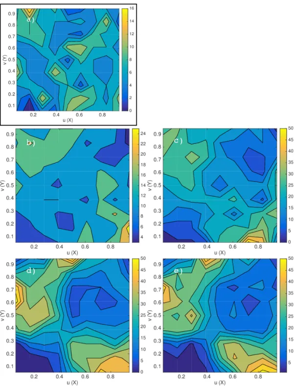
Clear differences can be seen between both stations, indicating different regimes and precipitation-generation processes. From Figure 4, it can be seen that, for LAMU station, low precipitation values are not strongly related to low rainfall rates. The same holds true for high values. Enhanced densities can be found for low rainfall rates and high temperatures. Such features can be partly reflected by only a few of the analyzed parameterization simulations. From Figure4, for instance, it becomes obvious that WRF-BLA, with its highest density at low precipitation and large temperature values, is not an optimal choice to represent the observed data. Additionally, it can be seen that the same cumulus parameterization scheme (here, Kain–Fritsch) leads to similar empirical copula density functions.
Atmosphere2019,10, 150 8 of 14
Version March 7, 2019 submitted toAtmosphere 8 of 14
Figure 4.Empirical Copula (defined on 9 x 9 lattice) of the P&T pairs at LAMU station (X: precipitation, Y: temperature) from a) observations, b) WRF-BLA, c) WRF-GWA, d) WRF-KLA, and e) WRF-KWA. Note the colorbar is not standardized, so as to better recognize the structures in the relatively flat Copulas.
accept theh1hypothesis (the modeled and observed P&T data come from different distributions). 197
Based on the retainedp-values of theχ2-test, one would select the BLA parametrization for LAMU, and 198
Figure 4. Empirical copula (defined on a 9×9 lattice) of thePandTpairs at LAMU station (X: precipitation,Y: temperature) from (a) observations, (b) WRF-BLA, (c) WRF-GWA, (d) WRF-KLA, and (e) WRF-KWA. Note that the color bar is not standardized, so as to better recognize structures in relatively flat copulas.
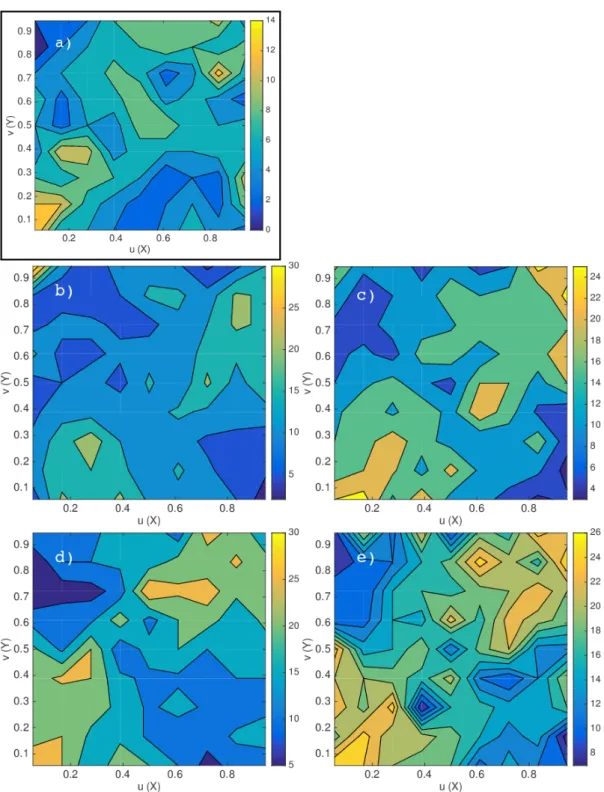
Figure 5.Same as Figure4, but for station MERU.
the KWA for MERU. It can be seen that the test result may depend on the lattice applied to estimate the 199
empirical Copula densities, which, in turn, depends on the number of data tuples available. Classically 200
(the separate evaluations of P&T), one would have come to a different selection (Table3). For station 201
MERU, one would have selected KLA for both precipitation and temperature, whereas one would 202
rather select BLA for precipitation and KWA for temperature. 203
Figure 5.Empirical Copula (defined on 9×9 lattice) of the P&T pairs at MERU station (X: precipitation,
Y: temperature) from (a) observations, (b) WRF-BLA, (c) WRF-GWA, (d) WRF-KLA, and (e) WRF-KWA. Note the colorbar is not standardized, so as to better recognize the structures in the relatively flat Copulas.
3.2. Selection of a Suitable WRF Parameter Combination
Besides visual inspection,χ2-test statistics were calculated so as to more objectively decide which
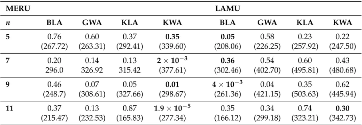
parameterization scheme should be selected. Table2displays the minimump-values for which theh0 hypothesis (the modeledPandTdata come from the same distribution as the observed data) can be rejected, i.e., small values close to zero cast doubt on independence. In this case, one would accept theh1hypothesis (modeled and observedPandTdata come from different distributions). Based on
Atmosphere2019,10, 150 10 of 14
the retainedp-values of theχ2-test, one would select BLA parameterization for LAMU, and KWA for
MERU. It can be seen that the test result may depend on the applied lattice to estimate the empirical copula densities, which, in turn, depends on the number of available data tuples. Classically (separate evaluations ofPandT), one would have come to a different selection (Table3). For MERU station, one would have selected KLA for both precipitation and temperature, whereas one would select BLA for precipitation and KWA for temperature.
Table 2.p- andχ2-values (brackets) ofχ2-tests for MERU and LAMU stations (2005–2009), conducted for various lattice dimensionsn×n. Smallest values are bolded.
MERU LAMU
n BLA GWA KLA KWA BLA GWA KLA KWA
5 0.76 0.60 0.37 0.35 0.05 0.58 0.23 0.22 (267.72) (263.31) (292.41) (339.60) (208.06) (226.25) (257.92) (247.50) 7 0.20 0.14 0.13 2×10⁻³ 0.36 0.54 0.60 0.43 296.0 326.92 315.42 (377.61) (302.46) (402.70) (495.81) (480.68) 9 0.46 0.07 0.05 0.01 4×10⁻³ 0.04 0.35 0.62 (248.7) (308.61) (327.66) (298.67) (261.36) (421.15) (503.63) (445.94) 11 0.37 0.13 0.87 1.9×10⁻⁵ 0.35 0.34 0.74 0.30 (215.47) (232.53) (165.83) (277.34) (166.12) (299.18) (323.21) (342.73) Table 3. Performance statistics assessed forPandT(Tis given in brackets) for MERU and LAMU stations without and with bias correction, conducted for the independent validation period (2011–2014). Smallest values are bolded.
MERU BLA GWA KLA KWA
MAE w/o BC 14.54 (2.30) 12.45 (2.74) 12.26(2.31) 12.83 (2.91) BC 15.25 (5.48) 13.70(4.36) 17.05 (4.77) 15.62 (4.85) MSE w/o BC 901.03 (7.55) 660.26 (9.71) 607.32(6.93) 641.13 (10.32) BC 856.57 (45.51) 638.67(34.38) 809.99 (37.71) 745.14 (16.57) RMSE w/o BC 30.02 (2.75) 25.70 (3.12) 24.64(2.63) 25.32 (3.21) BC 29.27 (6.75) 25.27(5.86) 28.46 (6.14) 27.30 (6.20)
LAMU BLA GWA KLA KWA
MAE w/o BC 9.20 (2.94) 8.05(3.34) 10.84 (3.29) 12.01 (2.01) BC 10.26 (0.86) 8.01(0.88) 8.11 (0.86) 9.01 (0.84) MSE w/o BC 233.67(9.70) 353.18 (12.22) 300.87 (11.72) 400.17 (4.85) BC 277.96 (1.18) 265.70 (1.22) 179.64(1.16) 244.89 (1.12) RMSE w/o BC 15.29(3.11) 18.79 (3.50) 17.35 (3.42) 20.00 (2.20) BC 16.67 (1.09) 16.30 (1.11) 13.40(1.08) 15.65 (1.06) 3.3. MOS Impact on Different WRF Parameterization Simulations
Two different types of MOS were applied to the WRF parameterization simulations, namely, local intensity scaling for precipitation and linear scaling for temperature. For precipitation, the selected-best configuration could not significantly be improved by the MOS; in fact, in most cases, statistics became worse. The same tendencies could also be observed for temperature and MERU station. For LAMU, however, temperature statistics could still be improved for the selected best configuration by the MOS. Interestingly, the MOS could not improve the performance statistics of any configuration suggested by joint selection (based on the empirical copulas). For the parameterization combinations suggested by the empirical copulas, namely, KWA for MERU and BLA for LAMU, performance decreased after application of the MOS approaches, except for LAMU temperature values. Here, the MOS lead to a remarkable improvement, which is very close to the best performing configuration (KWA). This indicates that the joint selection may lead to a better decision than traditional selection
does. By means of simple linear MOS, the temperature biases of the identified combination obtained by the joint selection approach (BLA) could be significantly reduced. In-depth analyses of the impact of different bias-correction schemes go beyond the scope of this study, but will be the subject of subsequent analyses.
4. Discussion
Multiphysics ensemble RCM studies traditionally focus on the representation of the statistics of single hydrometeorological variables (e.g., References [9,10,14,18,41–43]). As demonstrated by the present paper, this may lead to nonoptimal decisions on the parameterization combination with which to conduct RCM projections, induced by various performance measures for different hydrometeorological target variables.
Unlike the traditional selection procedure, the new joint evaluation approach specifically takes into account the covariance structure of RCM simulation variables such asPandT. Through this, the new approach can provide useful complementary knowledge for the identification of a suitable configuration combination. It is suggested to analyze empirical copula functions rather than the bivariate density plots in the data space [44], because only an empirical copula discloses significant differences in the joint dependence structure of the variables. Besides visual inspection, theχ2-test
allows making an objective decision with respect to the (P and T) dependence structure. Results were found to be robust, with only little impact of the choice of the observed lattice. Note that a relatively large simulation period is required (significantly longer than one year) due to precipitation’s intermittent nature and the inapplicability of the empirical copula in the case ofP=0 [30].
It is speculated that the new approach may reduce the need for complex multivariate postprocessing bias-correction approaches. However, one should test whether simple linear scaling approaches could further reduce biases, as shown for temperature at LAMU, or if performance further decreases compared to uncorrected series, since additional errors and uncertainties are introduced by MOS [15,16]. More in-depth studies are necessary to systematically check this speculation. Therefore, it is suggested to apply various MOS approaches with different levels of complexity and many more observation sites for validation than used in this conceptual study.
We conclude that the presented approach is a useful complement (besides traditional univariate evaluations) to identify suitable RCM physical parameterization combinations in order to obtain more reliable RCM simulations. Unlike the classical approach, it avoids ambiguity, since only one performance measure is considered, i.e.,χ2-test statistics. The new approach, however, should only
be considered as supplementary analysis. Classical approaches remain essential in the selection process, since they, e.g., also consider bias structures in a spatial sense rather than conduct pointwise evaluations. In theory, more variables thanPandTcould be implemented, depending on the needs and the available observation data.
Finally, the combination of the classical and the new joint evaluation approach may help to produce more reliable future climate projections, and may, therefore, contribute to the improvement of future climate-impact studies.
Author Contributions:Conceptualization, P.L.; methodology, P.L.; data curation, N.K.; writing—original-draft preparation, P.L.; writing—review and editing, H.K. and N.K.; visualization, P.L.; project administration, H.K.; funding acquisition, H.K. and P.L.
Funding:This study was partially funded by the Bavarian State Ministry for the Environment and Consumer Protection in the framework of the BIAS-II project (TKP01KPB-66747). N. Kerandi obtained funds from the National Commission for Science, Technology, and Innovation, and the German Academic Exchange Service. Acknowledgments:We appreciate the provision of computing resources from the Leibniz Supercomputing Center to conduct RCM simulations, and the ERA-Interim reanalysis data from the European Center for Medium-Range Weather Forecasts. Modelled and observedPandTtuples are available atftp://lauxpa.synology.me/FTP/RCM_ physics_parametrization_data/, provided by the Kenya Meteorological Services. We acknowledge support by Deutsche Forschungsgemeinschaft and Open Access Publishing Fund of Karlsruhe Institute of Technology.
Atmosphere2019,10, 150 12 of 14
Conflicts of Interest:The authors declare no conflict of interest. The funders had no role in the design of the study; in the collection, analyses, or interpretation of data; in the writing of the manuscript; or in the decision to publish the results.
References
1. Oettli, P.; Sultan, B.; Baron, C.; Vrac, M. Are regional climate models relevant for crop yield prediction in West Africa?Environ. Res. Lett.2011,6, 014008. [CrossRef]
2. Bronstert, A.; Kolokotronis, V.; Schwandt, D.; Straub, H. Comparison and evaluation of regional climate scenarios for hydrological impact analysis: General scheme and application example.Int. J. Climatol.2007,
27, 1579–1594. [CrossRef]
3. Maraun, D.; Wetterhall, F.; Ireson, A.M.; Chandler, R.E.; Kendon, E.J.; Widmann, M.; Brienen, S.; Rust, H.W.; Sauter, T.; Themel, M.; et al. Precipitation downscaling under climate change: Recent developments to bridge the gap between dynamical models and the end user.Rev. Geophys.2010,48. [CrossRef]
4. Berg, P.; Moseley, C.; Haerter, J.O. Strong increase in convective precipitation in response to higher temperatures.Nat. Geosci.2013,6, 181–185. [CrossRef]
5. Trenberth, K.E.; Shea, D.J. Relationships between precipitation and surface temperature.Geophys. Res. Lett.
2005,32, 1–4. [CrossRef]
6. Qiao, F.; Liang, X.-Z. Effects of cumulus parameterization closures on simulations of summer precipitation over the continental United States.J. Adv. Model. Earth Syst.2016,8, 764–785. [CrossRef]
7. Rasmussen, D.J.; Holloway, T.; Nemet, G.F. Opportunities and challenges in assessing climate change impacts on wind energy—A critical comparison of wind speed projections in California. Environ. Res. Lett.2011,
6, 024008. [CrossRef]
8. Van Oldenborgh, G.; Doblas Reyes, F.; Drijfhout, S.; Hawkins, E. Reliability of regional climate model trends.
Environ. Res. Lett.2013,8, 7. [CrossRef]
9. Evans, J.P.; Ekström, M.; Ji, F. Evaluating the performance of a WRF physics ensemble over South-East Australia.Clim. Dyn.2012,39, 1241–1258. [CrossRef]
10. Jerez, S.; Montavez, J.P.; Gomez-Navarro, J.J.; Lorente-Plazas, R.; Garcia-Valero, J.A.; Jimenez-Guerrero, P. A multi-physics ensemble of regional climate change projections over the Iberian Peninsula.Clim. Dyn.2013,
41, 1749–1768. [CrossRef]
11. Laux, P.; Lorenz, C.; Thuc, T.; Ribbe, L.; Kunstmann, H. Setting up regional climate simulations for Southeast Asia. InHigh Performance Computing in Science and Engineering ’12; Springer: Berlin/Heidelberg, Germany, 2013; pp. 391–406. [CrossRef]
12. Casanueva, A.; Herrera, S.; Fernández, J.; Frías, M.D.; Gutiérrez, J.M. Evaluation and projection of daily temperature percentiles from statistical and dynamical downscaling methods.Nat. Hazards Earth Syst. Sci.
2013,13, 2089–2099. [CrossRef]
13. Solman, S.A.; Pessacg, N.L. Regional climate simulations over South America: Sensitivity to model physics and to the treatment of lateral boundary conditions using the MM5 model.Clim. Dyn.2012,38, 281–300. [CrossRef]
14. Katragkou, E.; Garciá-Diéz, M.; Vautard, R.; Sobolowski, S.; Zanis, P.; Alexandri, G.; Cardoso, R.M.; Colette, A.; Fernandez, J.; Gobiet, A.; et al. Regional climate hindcast simulations within EURO-CORDEX: Evaluation of a WRF multi-physics ensemble.Geosci. Model Dev.2015,8, 603–618. [CrossRef]
15. Ehret, U.; Zehe, E.; Wulfmeyer, V.; Warrach-Sagi, K.; Liebert, J. HESS Opinions “Should we apply bias correction to global and regional climate model data?”. Hydrol. Earth Syst. Sci. 2012, 16, 3391–3404. [CrossRef]
16. Ramirez-Villegas, J.; Challinor, A.J.; Thornton, P.K.; Jarvis, A. Implications of regional improvement in global climate models for agricultural impact research.Environ. Res. Lett.2013,8, 024018. [CrossRef]
17. Pohl, B.; Crétat, J.; Camberlin, P. Testing WRF capability in simulating the atmospheric water cycle over Equatorial East Africa.Clim. Dyn.2011,37, 1357–1379. [CrossRef]
18. Endris, H.S.; Omondi, P.; Jain, S.; Lennard, C.; Hewitson, B.; Chang’a, L.; Awange, J.L.; Dosio, A.; Ketiem, P.; Nikulin, G.; et al. Assessment of the performance of CORDEX regional climate models in simulating East African rainfall.J. Clim.2013,26, 8453–8475. [CrossRef]
19. Kerandi, N.M.; Laux, P.; Arnault, J.; Kunstmann, H. Performance of the WRF model to simulate the seasonal and interannual variability of hydrometeorological variables in East Africa: A case study for the Tana River basin in Kenya.Theor. Appl. Climatol.2016,130, 401–418. [CrossRef]
20. Zittis, G.; Hadjinicolaou, P.; Lelieveld, J. Comparison of WRF Model Physics Parameterizations over the MENA-CORDEX Domain.Am. J. Clim. Chang.2014,3, 490–511. [CrossRef]
21. Zittis, G.; Hadjinicolaou, P. The effect of radiation parameterization schemes on surface temperature in regional climate simulations over the MENA-CORDEX domain. Int. J. Climatol. 2017, 37, 3847–3862. [CrossRef]
22. Kerandi, N.M.; Arnault, J.; Laux, P.; Wagner, S.; Laux, P.; Kitheka, J.; Kunstmann, H. Joint atmospheric–terrestrial water balances for East Africa: A WRF-Hydro case study for the upper Tana River basin.Theor. Appl. Climatol.2017. [CrossRef]
23. Betts, A.K. A new convective adjustment scheme. Part I: Observational and theoretical basis. Q. J. R. Meteorol. Soc.1984,112, 693–709.
24. Lin, Y.-L.; Farley, R.D.; Orville, H.D. Bulk Parametrization of the Snow Field in a Cloud Model.
J. Appl. Meteorol.1983,22, 1065–1092. [CrossRef]
25. Pleim, J.E. A combined local and nonlocal closure model for the atmospheric boundary layer. Part I: Model description and testing.J. Appl. Meteorol. Climatol.2007,46, 1383–1395. [CrossRef]
26. Grell, G.A.; Freitas, S.R. A scale and aerosol aware stochastic convective parameterization for weather and air quality modeling.Atmos. Chem. Phys.2014,14, 5233–5250. [CrossRef]
27. Hong, S.; Lim, J. The WRF single-moment 6-class microphysics scheme (WSM6).J. Korean Meteor. Soc.2006,
42, 129–151.
28. Kain, J.S.; Fritsch, J.M. A One-Dimensional Entraining Detraining Plume Model and Its Application in Convective Parameterization.J. Atmos. Sci.1990,47, 2784–2802. [CrossRef]
29. Van Den Berg, M.J.; Vandenberghe, S.; De Baets, B.; Verhoest, N.E.C. Copula-based downscaling of spatial rainfall: A proof of concept.Hydrol. Earth Syst. Sci.2011,15, 1445–1457. [CrossRef]
30. Mao, G.; Vogl, S.; Laux, P.; Wagner, S.; Kunstmann, H. Stochastic bias correction of dynamically downscaled precipitation fields for Germany through copula-based integration of gridded observation data.Hydrol. Earth Syst. Sci.2015,11, 7189–7227. [CrossRef]
31. Laux, P.; Vogl, S.; Qiu, W.; Knoche, H.R.; Kunstmann, H. Copula-based statistical refinement of precipitation in RCM simulations over complex terrain.Hydrol. Earth Syst. Sci.2011,15, 2401–2419. [CrossRef]
32. Vogl, S.; Laux, P.; Qiu, W.; Mao, G.; Kunstmann, H. Copula-based assimilation of radar and gauge information to derive bias-corrected precipitation fields.Hydrol. Earth Syst. Sci.2012,16, 2311–2328. [CrossRef] 33. Lorenz, C.; Montzka, C.; Jagdhuber, T.; Laux, P.; Kunstmann, H. Long-term and high-resolution global time
series of brightness temperature from copula-based fusion of SMAP enhanced and SMOS data.Remote Sens.
2018,10, 1842. [CrossRef]
34. Nelsen, R.B.An Introduction to Copulas; Springer: New York, NY, USA, 1999.
35. Sklar, A. Fonctions de Répartition à n Dimensions et Leurs Marges. InPublications de l’Institut Statistique de l’Université de Paris; Institut Henri Poincaré: Paris, France, 1959; Volume 8, pp. 229–231.
36. Deheuvels, P. Point processes and multivariate extreme values.J. Multivar. Anal.1983,13, 257–272. [CrossRef] 37. Genest, C.; Rémillard, B.; Beaudoin, D. Goodness-of-fit tests for copulas: A review and a power study.
Insur. Math. Econ.2009,44, 199–213. [CrossRef]
38. Wilks, D.Statistical Methods in the Atmospheric Sciences, 2nd ed.; Academic Press: Cambridge, MA, USA, 2011; p. 467. [CrossRef]
39. Leander, R.; Buishand, T.A. Resampling of regional climate model output for the simulation of extreme river flows.J. Hydrol.2007,332, 487–496. [CrossRef]
40. Schmidli, J.; Frei, C.; Vidale, P.L. Downscaling from GCM precipitation: A benchmark for dynamical and statistical downscaling methods.Int. J. Climatol.2006,26, 679–689. [CrossRef]
41. Argüeso, D.; Hidalgo-Muñoz, J.M.; Gámiz-Fortis, S.R.; Esteban-Parra, M.J.; Dudhia, J.; Castro-Díez, Y. Evaluation of WRF parameterizations for climate studies over southern Spain using a multistep regionalization.J. Clim.2011,24, 5633–5651. [CrossRef]
42. García-Díez, M.; Fernández, J.; Fita, L.; Yagüe, C. Seasonal dependence of WRF model biases and sensitivity to PBL schemes over Europe.Q. J. R. Meteorol. Soc.2013,139, 501–514. [CrossRef]
Atmosphere2019,10, 150 14 of 14
43. Di Luca, A.; Flaounas, E.; Drobinski, P.; Brossier, C.L. The atmospheric component of the Mediterranean Sea water budget in a WRF multi-physics ensemble and observations.Clim. Dyn.2014,43, 2349–2375. [CrossRef] 44. Piani, C.; Haerter, J.O. Two dimensional bias correction of temperature and precipitation copulas in climate
models.Geophys. Res. Lett.2012,39, 6. [CrossRef] c
2019 by the authors. Licensee MDPI, Basel, Switzerland. This article is an open access article distributed under the terms and conditions of the Creative Commons Attribution (CC BY) license (http://creativecommons.org/licenses/by/4.0/).