DOAM for Evolutionary Portfolio Optimization: a computational study.

(1)

Dipartimento di Scienze Economiche, Matematiche e Statistiche

Università degli Studi di Foggia

____________________________________________________________________

DOAM for Evolutionary Portfolio Optimization: a

computational study

Gabriella Dellino, Mariagrazia Fedele e Carlo

Meloni

Quaderno n. 05/2008

“Esemplare fuori commercio per il deposito legale agli effetti della legge 15 aprile 2004 n. 106”

Quaderno riprodotto al

Dipartimento di Scienze Economiche, Matematiche e Statistiche

nel mese di marzo 2008 e

depositato ai sensi di legge

Authors only are responsible for the content of this preprint.

_______________________________________________________________________________

Dipartimento di Scienze Economiche, Matematiche e Statistiche, Largo Papa Giovanni Paolo II, 1,

(2)

DOAM for Evolutionary Portfolio Optimization:

a computational study.

Gabriella Dellino∗_{, Mariagrazia Fedele}†_{, and Carlo Meloni}‡ February 8, 2008

Abstract

In this work, the ability of the Dynamic Objectives Aggregation Methods to solve the portfolio rebalancing problem is investigated con-ducting a computational study on a set of instances based on real data. The portfolio model considers a set of realistic constraints and entails the simultaneously optimization of the risk on portfolio, the expected return and the transaction cost.

1 Introduction

The standard problem of portfolio selection consists in allocating wealth among available investments. Letnbe the number of available risky assets with expected returnsµi and variancesσii; letσij be the covariance between

the asset i and the asset j and Σ = (σij) be the covariance matrix. We

denote with xi the proportion of the capital to be allocated to the asset

i. Therefore, the standard problem of portfolio selection can be stated as follows: min x0Σx, (Min-Risk) (1) subject to µ0x=µ, (2) x01 = 1, (3) xi ≥0, i= 1, . . . , n; (4)

The solution of the previous problem is the portfolio with minimum risk among those with a fixed expected returnµ. Equations (3) and (4) represent

∗_{Dipartimento di Matematica, Universit`a di Bari, Via E. Orabona, 4 - 70125 Bari.} †_{Dipartimento di Scienze Economiche, Matematiche e Statistiche, Universit`a di Foggia,} Largo Papa Giovanni Paolo II, 1 - 71100.

‡_{Dipartimento di Elettrotecnica ed Elettronica, Politecnico di Bari, Via E. Orabona, 4} - 70125 Bari.

(3)

the balance constraint and the non-negative constraint, respectively; the latter is left out when short sales are allowed. Mean-variance approach allows to trace out the efficient frontier, a set of portfolios that offer the minimum risk level for a given level of reward. The shape of the efficient set differs according to the assumptions in regard to the ability of the investor to sell security short as well as the ability to lend and to borrow funds. The scenario of the classical mean-variance model is an ideal market: no transaction costs, no holding constraints, no limit on portfolio cardinality, no regulatory requirements are present. Since any realistic portfolio problem has to take into account these practical issues, it is necessary to consider a model including costs and constraints. The introduction of such constraints, particularly cardinality range, raises the computational complexity of the portfolio model which turns out to beN P-hard.

In this work, a computational and comparative study on the application of DOAMs on multi-objective rebalancing problem is proposed. Section 2 presents the portfolio rebalancing problem and describes the transaction costs and the multi-objective rebalancing model. In section 3 the Dynamic Objective Aggregation Methods are briefly introduced and the experimental setting is described; section 4 presents the analysis of results, while in the last section some comments are drawn.

2 Portfolio Rebalancing problem

Let us consider now the revision of the current portfoliox0_{; let the}_n_vector

x0 = (x0₁, . . . , x_n0) be the current portfolio and let x = (x1, . . . , xn) be the

portfolio after rebalance; x is a vector of fraction of the capital invested in each asset, therefore the vector of amount of money actually invested is Cx, where C stands for the available capital or, in rebalancing problem, the value of the current portfolio x0_{. In any realistic portfolio rebalancing} the investors have to face transaction costs; letTx

x0 be the transaction cost

associated with the rebalance fromx0 _to_x_; _Tx

x0 is a function of the vector

of the trading volumesv=|x−x0_|C_:

vi=

½

(xi−x0i)C if the exposure to the iasset is increased by purchases,

(x0

i −xi)C if the exposure to the iasset is reduced by sales.

In our model we assume that the transaction costs both for purchases and sales are equal. Furthermore, it is assumed that the cost function is a separable function: T_xx₀(v) = n X i=1 t_i(v_i).

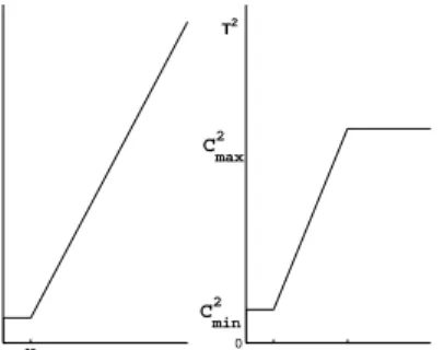
We are considering small size of trade; in particular, from trading online transaction costs we derive two type of transaction function according to

(4)

the type of securities,t1 i andt2i: t1_i(vi) = ½ 0 ifxi =x0i max{c1 min, c1irvi} otherwise (5) t2_i(vi) = ( 0 ifx_i =x0 i min ³ max{c2 min, c2irvi},c2max ´ otherwise (6) wherec1

min and c2min denotes the minimum costs,c2max the maximum costs,

c2r

i and c1ir stand for the commission rates for the asseti. The first trading

function entails a fixed cost until a given level of amount tradedv1_{; beyond}

v1 the costs increase linearly with the volume transacted. In the second function, there is an upper bound on the transaction costs, as well: beyond an upper levelv2 _{the transaction costs are fixed. The model proposed is the}

0 _v 0 1 _v 1 v2 C1 min C 2 min C2 max T1 T2

Figure 1: Transaction cost function following: min x0Σx, max x0µ, (7) min n X i=1 t_i(|x_i−x0_i|C) x01 = 1, K1≤ n X i=1 Zi ≤K2, liZi≤xi ≤uiZi, i∈ {1, . . . , n} Zi∈ {0,1}, i∈ {1, . . . , n}.

ti denotes the cost function of the asseti;K1 and K2 are the minimum and maximum number of assets that must be in portfolio; li and ui are lower

(5)

3 DOAMs’ Configuration

To solve the portfolio rebalancing problem as a multi-criteria optimization problem, a dynamic scalarization method based on different aggregate func-tions in an evolutionary optimization scheme is used. The Dynamic Ob-jective Aggregation Methods are based on the standard genetic algorithm included in the Matlab’s Genetic Algorithm and Direct Search Toolbox [7]. These algorithms with different rules of weights changing have been first tested on benchmark problems from the literature and compared with a widely used standard multi-objective algorithm: NSGA-II [3]. Computa-tional results of this preliminary campaign of experiments are reported in [4]. The algorithms achieving better results are employed in a second cam-paign of experiments devoted to tackle the multi-objective portfolio rebal-ancing problem; therefore, we investigate the ability of the heuristic DOAMs to solve the portfolio rebalancing model. Among the 24 DOAMs tested in the preliminary study [4], obtained combining the weights generation rules and the four strategies considered for the variation of the exponents, the best 6 algorithms are chosen, namely: chaotic, sinusoidal and triangular weights generators are combined with exponents fixed to one (Chaos-Gen,

Sin-Gen, Trian-Gen) and with the adaptive scheme (Chaos+Exp, Sin+Exp,

Trian+Exp). In the adaptive scheme the exponent value is incremented

when there is no improvement in the optimization process for a given num-ber of iterations, which has been fixed to ∆ = 0.05N, beingN the maximum number of generations that can be produced.

In the preliminary computational study [4], we used the DOAMs for two-objective problems; as the model (7) has three two-objectives, the aggregate function has the following expression

F(x, k) =w1(k)f1t(x) +w2(k)f2t(x) +w3(k)f3t(x).

The weights w_k are dynamically modified according to a function R(k) of the generation number k:

w1(k) =R(k), w2(k) = (1−w1)w1, w3(k) = 1−w1−w2. A periodical changing of the weights can be obtained according to a sin or triangle wave; the sinusoidal rule is the following:

R(k) =|sin(2πk/F)|, (8)

where F is the frequency and it has been fixed to F = 200. Whereas, a chaotic variation law to the weights is employed as follows:

w1(k+ 1) =µw1(k)(1−w1(k)). (9) Whenµ= 4 and w1(0)6∈ {0,0.25,0.5,0.75,1}, the previous equation shows chaotic behaviour.

(6)

As the DOAMs are based on the standard genetic algorithm included in the Matlab’s Genetic Algorithm and Direct Search Toolbox, some parameters values need to be specified, before the algorithm execution: we adopted a stochastic uniform selection operator, a scattered crossover function with probability 0.7 and a Gaussian mutation function with probability 0.3; the number of best individuals that will survive to the next population has been fixed to 2.

The population size is of 100 individuals; the archive used is made up of 500 individuals.

In our experiments, we consider two different stopping criteria: in the first set of computational tests the stopping criterion is based on the maximum number of generations to be produced and it is fixed to 500; therefore the computational time can be considered as a performance indicator. Since from the first results it seems evident that the DOAMs are faster than the NSGA-II, the computational tests are then repeated considering the execution time as stopping criterion, i.e. a time limit of 600 seconds is adopted.

3.1 Cardinality and Holding Constraints

Since the DOAMs are population based algorithms, at each generation a population of individuals (children) or solutions are produced by genetic operators of selection, crossover and mutation from the previous genera-tion (parents). Not all possible individuals correspond to feasible portfolios, because of the holdings and cardinality constraints; therefore a procedure provided by Changet al., [2] is used to assure the individuals to be always feasible.

Let us consider n real numbers si,0 ≤ si ≤ 1, i= 1, . . . , n; let the vector

(s₁, . . . , s_n) be an individual (child) of the population generated by the algo-rithm. Considering the setQ={is.t. si 6= 0} ⊂ {1, . . . , n},K=|Q|is the

number of non-zero elements of the individual (s1, . . . , sn). If K is greater

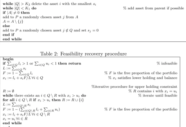
than K₁ and lower then K₂, then the individual satisfies the cardinality constraint; otherwise a procedure to assure the cardinality constraints are satisfied is used. This procedure is described in the pseudo-code 1:

After we have assured that the number of non-zero s_i is between K₁

and K2, we use a procedure to assure that the holding and the balance constraints are satisfied too. This procedure is shown in a pseudo-code in Table 2.

3.2 Portfolio Data Set

The comparison of different DOAMs implementations is performed on a set of instances based on a public data set provided by Beasley and available from OR-Library [1].

(7)

Table 1: Procedure for the fulfillment of cardinality constraints

Athe set of assets that are in the parents, but are not in the child

P the set of assetsiwithi∈Q,

while|Q|> K2 delete the assetiwith the smallestsi

while|Q|< K1 do % add asset from parent if possible

if|A| 6= 0then

add toP a randomly chosen assetjfromA A=A\ {j}

else

add toP a randomly chosen assetj /∈Qand setsj= 0 end if

end while

Table 2: Feasibility recovery procedure

begin

ifPi∈Qli>1 orPi∈Qui<1then return % infeasible

L:=P_i_∈_Qsi

F:= 1−Pi∈Qli %F is the free proportion of the portfolio

xi:=li+siF/L∀i∈Q %xisatisfies lower holding and balance

%iterative procedure for upper holding constraint

R:=∅ %Rcontainsiwithxi=ui

whilethere exists ani∈Q\Rwithxi> uido % iterate until feasible

for alli∈Q\Rifxi> uithenR:=R∪ {i}

L:=P_i_∈_Q_\_Rsi

F:= 1−(P_i_∈_Q_\_Rli+

P

i∈Rui) %F is the free proportion of the portfolio

xi:=li+siF/L∀i∈Q\R

xi=ui∀i∈R end while end

The financial data sets (means and variance matrix) are constructed using the stocks involved in five capital market indices. The weekly prices from March 1992 to September 1997 are taken into account for the stocks of Hang Seng (Hong Kong), DAX 100 (Germany), FTSE 100 (UK), SP 100 (USA) and Nikkei 225 (Japan). The size of the five tests problems varies from

n= 31 (Hang Seng) ton= 225 (Nikkei).

We extended the Beasley’s original instances introducing our more realis-tic aspects in both objectives and constraints. We use the two transaction costs structures defined by equations (5), (6). The data used for the param-eters characterizing the commission costs are realistic values obtained from available trading online data:

c1_min= 15, c1r

i = 0.30%,

c2_min= 2.5, c_i2r= 0.20%, c2_max= 20.

Two different configurations of constraints are considered:

Configuration 1 : K1= 9, K2= 11, K0 = 10, li= 0.05, ui= 0.75,

(8)

Combining the two transaction cost functions with the two constraints’ con-figurations, 4 overall different formulations of the problems are considered. In the conducted experiments we assume the invested capitalC = 100000, while the initial portfolios are generated randomly.

4 Computational Results

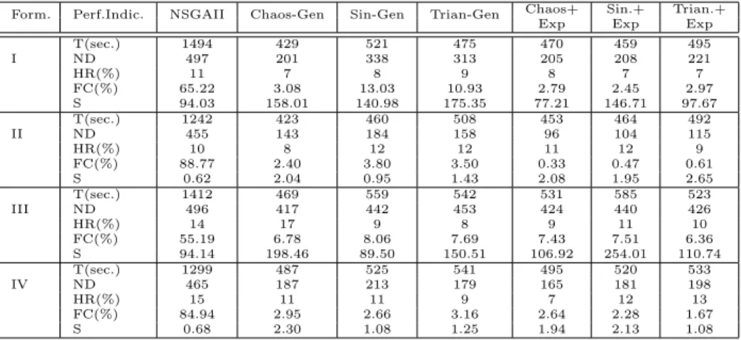
To compare the different DOAMs on portfolio instances, we use four per-formance indexes; we consider the hyperarea ratio (HR), and the number of non-dominated elements setting up the efficient frontier (ND); we report the fractional contribution (FC) defined as the percentage of non dominated points contributed by an algorithm on the total efficient frontier obtained unifying all the efficient sets produced by all the algorithms on the same instance. Precisely, the total efficient frontier is obtained unifying all the efficient frontier and executing a dominance analysis: dominated points or eventually double points are removed. The fractional contribution is cal-culated as the number of points achieved by an algorithm that are present in the total front, out of the number of solutions in total frontier. As last indicator, we report the spacing (S).

Since the first experiments are made using the number of iterations as stop-ping criterion, we can consider the computational time (T) as performance indicator. As in the second set of experiments a time limit of 600 seconds is adopted, the number of generations (G) is also reported as performance index.

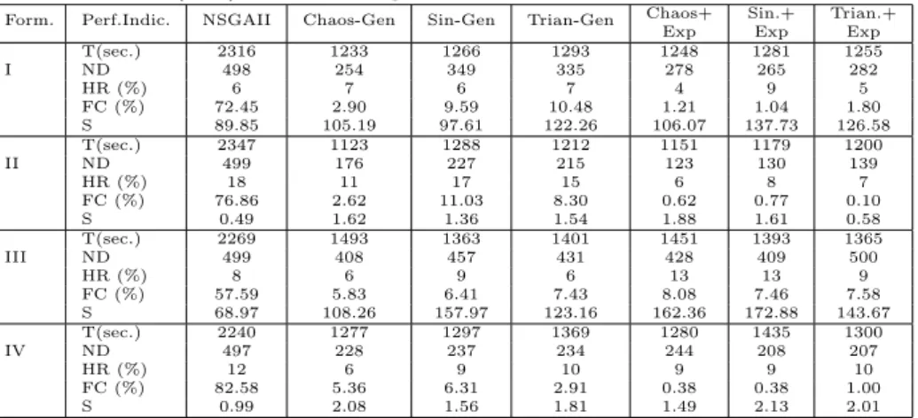
For each experiment three different runs have been executed initializing al-gorithms with random populations; therefore the values of performance indi-cators have to be considered as mean values. Tables 3 - 7 contain the average results on 3 runs for each of the 4 algorithms configurations described; the computational results reported are obtained for the five portfolio problems with the stopping criterion of 500 iterations. Tables 8 - 12 contain the av-erage results on 3 runs for each algorithms configurations obtained with a time limit of 600 seconds.

From the first campaign of experiments, as global observation, we can say that all the DOAMs present a promising behavior, but no dynamic objec-tives algorithm perform always better than others. Furthermore, it can be observed that the DOAMs are, on the whole, faster than the NSGA-II for every instance and for every problem. While the fractional contribution FC of the NSGA-II is generally greater than that one of the DOAMS, the val-ues of the main performance index, i.e. the hyperarea ratio, do not present relevant differences on the average.

Similar arguments can be used also in the experiments made with a fixed computation time. It can be observed that, although the NSGA-II presents again much more high percentages of fractional contributes and higher

(9)

num-ber of nondominated points, the hyperarea values of the DOAMs are compa-rable with that one of NSGA-II, and in several cases they are even better. In particular, in the 20,8% and 23,3% of cases DOAMs outperform NSGA-II in the first and second group of experiments, respectively. The compara-tive evaluation on this computational campaign of experiments restricted to DOAMs shows Trian-Gen and Sin-Gen and their t-power counterparts as better strategies.

5 Concluding Considerations

We have provided a reliable and general, yet improvable, algorithmic instru-ment to solve realistic objective optimization problems. The multi-objective approach allows us to solve re-weighting portfolio problem also minimizing transaction costs. The proposed resolution methods based on evolutionary schemes and working with populations of solutions result - af-ter different campaigns of experiments - to be a suitable instrument to solve multi-objective problems. Eventually other objectives can be taken into ac-count in the portfolio problem without the algorithmic approach is changed. Future researches may be done both on the portfolio model and on the algorithmic methods. Since we have considered only the commissions’ com-ponent of the transaction costs, the market impact cost could be considered. From the algorithmic point of view, in order to exploit the speed of DOAMs, an algorithm combining NSGA-II (or another standard population-based multi-objective algorithm) with a DOAM as local search algorithm deserves to be experimentally evaluated.

Moreover, other DOAMs with different aggregating functions can be con-sidered: in addition to the t-power transformation, e.g. Lin et al. in [5] investigated the exponential transformation of the objective functions and its capability to convexify the efficient frontier.

The analysis of the impact of algorithm’s parameters on the achievable com-putational performance is another topic for further research. It could be devoted to point out suitable procedures for the fine tuning of these param-eters.

References

[1] Beasley J. E.: OR-Library: distributing test problems by electronic mail. Journal of the Operation Research Society, 41, pp. 1069-72, 1990. [2] Chang T.-J., Meade N., Beasley J. E., Heuristics for cardinality

con-strained portfolio optimization, Computers Operation Research 27, pp.

(10)

[3] Deb K., Pratap A., Agarwal S. and Meyarivan T., A Fast and Elitist

Multiobjective Genetic Algorithm: NSGA-II, in IEEE Transactions on

Evolutionary Computation, Vol. 6, No. 2, pp. 182-197, 2002.

[4] Dellino G., Fedele M., Meloni C., Dynamic Objectives Aggregation in

Multi-objective Evolutionary Optimization Technical Report DEE -

Po-litecnico di Bari.

[5] Li D., Biswal M. P.,Exponential transformation in convexifying a

non-inferior frontier and exponential generating method, Journal of

Opti-mization Theory and Applications: Vol.99, No. 1, pp. 183-199, 1998. [6] Lin, D., Wang S., Yan H.,A multiobjective genetic algorithm for

port-folio selection problem, Proceedings of ICOTA, 2001.

A multiobjective genetic algorithm for portfolio selection. Working Pa-per, Institute of Systems Science, Academy of Mathematics and Sys-tems Science Chinese Academy of Sciences, Beijing, China.

[7] The MathWorks Inc., Genetic Algorithm and Direct Search Toolbox, Natick, Massachussetts, 2004.

Table 3: Average values of T, ND, HR, FC and S for the portfolio problem 1 with a fixed (500) number of generations.

Chaos+ Sin.+ Trian.+ Form. Perf.Indic. NSGAII Chaos-Gen Sin-Gen Trian-Gen

Exp Exp Exp

T(sec.) 1494 429 521 475 470 459 495 I ND 497 201 338 313 205 208 221 HR(%) 11 7 8 9 8 7 7 FC(%) 65.22 3.08 13.03 10.93 2.79 2.45 2.97 S 94.03 158.01 140.98 175.35 77.21 146.71 97.67 T(sec.) 1242 423 460 508 453 464 492 II ND 455 143 184 158 96 104 115 HR(%) 10 8 12 12 11 12 9 FC(%) 88.77 2.40 3.80 3.50 0.33 0.47 0.61 S 0.62 2.04 0.95 1.43 2.08 1.95 2.65 T(sec.) 1412 469 559 542 531 585 523 III ND 496 417 442 453 424 440 426 HR(%) 14 17 9 8 9 11 10 FC(%) 55.19 6.78 8.06 7.69 7.43 7.51 6.36 S 94.14 198.46 89.50 150.51 106.92 254.01 110.74 T(sec.) 1299 487 525 541 495 520 533 IV ND 465 187 213 179 165 181 198 HR(%) 15 11 11 9 7 12 13 FC(%) 84.94 2.95 2.66 3.16 2.64 2.28 1.67 S 0.68 2.30 1.08 1.25 1.94 2.13 1.08

(11)

Exp Exp Exp

T(sec.) 2173 993 1019 1033 1088 1052 1085 I ND 496 154 177 171 168 171 190 HR(%) 10 3 11 12 5 6 3 FC(%) 78.82 1.32 5.76 5.76 0.87 2.05 3.91 S 27.39 108.50 241.20 355.41 162.25 180.05 151.65 T(sec.) 2067 991 985 1028 1019 1024 1064 II ND 495 106 110 104 86 793 827 HR(%) 6 6 7 8 6 6 5 FC(%) 87.06 2.22 7.39 2.93 0.11 0.11 0.17 S 0.45 2.30 1.50 2.75 2.54 2.24 2.75 T(sec.) 2078 1025 1087 1098 1043 1042 990 III N.pt 498 276 244 249 268 275 227 HR(%) 12 9 9 11 9 8 11 FC(%) 60.61 8.12 6.54 5.71 5.67 5.71 4.44 S 59.39 343.47 337.37 216.04 337.89 196.35 391.83 T(sec.) 1978 1042 1069 1198 1058 1106 1105 IV ND 492 123 123 105 121 125 131 HR(%) 20 5 5 6 6 5 6 FC(%) 88 1.12 2.14 2.85 1.31 1.32 1.61 S 0.55 4.25 2.76 3.16 2.42 3.10 3.07

Exp Exp Exp

T(sec.) 2316 1233 1266 1293 1248 1281 1255 I ND 498 254 349 335 278 265 282 HR (%) 6 7 6 7 4 9 5 FC (%) 72.45 2.90 9.59 10.48 1.21 1.04 1.80 S 89.85 105.19 97.61 122.26 106.07 137.73 126.58 T(sec.) 2347 1123 1288 1212 1151 1179 1200 II ND 499 176 227 215 123 130 139 HR (%) 18 11 17 15 6 8 7 FC (%) 76.86 2.62 11.03 8.30 0.62 0.77 0.10 S 0.49 1.62 1.36 1.54 1.88 1.61 0.58 T(sec.) 2269 1493 1363 1401 1451 1393 1365 III ND 499 408 457 431 428 409 500 HR (%) 8 6 9 6 13 13 9 FC (%) 57.59 5.83 6.41 7.43 8.08 7.46 7.58 S 68.97 108.26 157.97 123.16 162.36 172.88 143.67 T(sec.) 2240 1277 1297 1369 1280 1435 1300 IV ND 497 228 237 234 244 208 207 HR (%) 12 6 9 10 9 9 10 FC (%) 82.58 5.36 6.31 2.91 0.38 0.38 1.00 S 0.99 2.08 1.56 1.81 1.49 2.13 2.01

(12)

Exp Exp Exp

Table 8: Average values of G, ND, HR, FC and S with time fixed to 10 minutes for the portfolio problem 1.

Exp Exp Exp

G 223 602.33 573.67 572.67 666 678 685.33 ND 496 248 273 238 260 270 258 I HR (%) 20 14 12 14 12 12 12 FC (%) 67.99 5.55 5.14 5.22 4.23 4.64 5.66 S 25.94 75.45 117.63 135.15 108.89 146.53 325.56 G 278 604 600.33 611.33 715.33 689.33 721 ND 394 164 185 162 103 112 113 II HR (%) 29 27 25 28 24 22 24 FC (%) 78.37 6.04 7.10 6.16 0.69 0.69 1.16 S 0.55 1.22 1.25 1.13 1.70 1.34 1.71 G 211.67 462 467.67 469.33 505.33 496 489.67 ND 496 430 437 419 468 443 446 II HR (%) 23 10 10 18 13 12 11 FC (%) 53.01 6.89 7.52 8.36 7.76 7.36 7.69 S 61.03 86.27 154.89 201.22 121.19 153.87 130.12 G 241.33 531.67 525.67 528.33 570 580.33 633.33 ND 455 181 193 172 187 182 187 II HR (%) 15 10 11 12 10 11 12 FC (%) 83.51 2.85 4.68 1.61 1.80 1.91 2.14 S 0.50 1.84 1.24 1.51 1.67 1.03 2.30

Exp Exp Exp

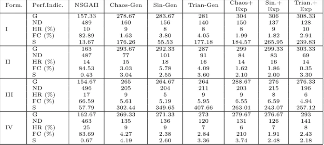
G 157.33 278.67 283.67 281 304 306 308.33 ND 489 160 156 140 150 137 128 I HR (%) 10 9 8 8 8 9 10 FC (%) 82.89 1.63 3.80 4.05 1.99 1.82 2.91 S 13.67 176.26 55.53 177.18 184.57 265.95 239.83 G 163 293.67 292.33 287 299 299.33 303.33 ND 487 77 101 91 84 83 69 II HR (%) 14 15 18 16 14 16 14 FC (%) 84.53 3.03 5.78 4.09 1.62 1.86 0.35 S 0.43 3.04 2.55 3.60 2.10 2.00 3.30 G 154.67 265 264.67 264 288.67 276 276.33 ND 496 205 204 211 203 215 196 III HR (%) 17 9 5 9 9 8 6 FC (%) 66.59 5.61 5.19 5.95 6.55 6.59 4.94 S 57.79 302.44 349.65 407.66 263.01 243.07 257.12 G 162.67 269.33 271.33 273 279.67 276.67 293 ND 463 135 136 120 131 126 141 IV HR (%) 25 9 9 7 6 7 8 FC (%) 83.69 4.27 2.38 2.84 210 1.91 2.43 S 0.67 4.19 2.60 3.36 3.74 2.48 2.18

(13)

Exp Exp Exp

G 154.67 271.33 280.67 268 297.67 295 297.67 ND 493 165 166 211 164 180 170 I HR (%) 22 11 12 14 14 14 16 FC (%) 70.10 3.83 4.75 6.31 4.69 5.09 4.20 S 51.01 313.49 322.60 184.93 272.19 183.89 139.44 G 158.67 275.33 279.67 284.67 290.33 297.67 296.33 ND 485 93 126 95 88 93 80 II HR (%) 20 20 19 24 20 22 22 FC (%) 86.69 2.52 5.73 2.98 0.91 0.67 1.17 S 0.53 4.67 0.98 5.66 4.98 4.35 3.50 G 149.33 242.33 245.67 247.33 258.67 254.67 257.67 ND 497 365 343 358 364 338 327 III HR (%) 17 13 10 15 8 11 10 FC (%) 49.70 9.22 8.11 8.74 8.08 7.40 7.71 S 119.62 329.52 324.19 303.40 236.53 242.83 353.28 G 158.67 264.67 268 266.33 276.33 269.67 291.33 ND 466 161 143 166 152 161 141 IV HR (%) 18 10 14 8 13 11 12 FC (%) 76.08 8.26 4.06 1.87 1.34 1.85 6.19 S 0.57 4.37 3.71 3.03 4.08 7.86 4.96

Exp Exp Exp

G 140.67 236.33 245.33 245.67 252.33 247.67 258 ND 496 248 215 219 224 231 218 I HR (%) 8 8 8 9 12 10 11 FC (%) 82.80 6.13 2.09 1.15 2.14 2.09 1.65 S 54.56 128.78 128.21 153.19 135.09 127.00 123.11 G 140 256.67 252.33 249.33 256 264.33 259.67 ND 495 135 158 145 96 119 100 II HR (%) 15 9 18 15 10 22 16 FC (%) 77.80 6.83 8.37 6.62 0.05 0.16 0.17 S 0.71 3.10 2.10 1.65 0.84 0.61 0.48 G 136.67 220.67 222.67 222.33 215.33 218 224 ND 496 359 311 357 348 376 377 III HR (%) 6 10 9 8 9 9 9 FC (%) 60.54 6.72 6.99 5.64 6.19 6.27 6.09 S 51.22 137.55 166.41 171.04 166.23 177.56 196.87 G 140.33 236.33 236.33 236.67 238.67 249.33 248 ND 494 201 175 210 226 200 213 IV HR (%) 12 9 8 7 8 8 7 FC (%) 77.45 2.25 3.06 5.43 4.47 4.32 3.68 S 0.89 1.55 2.17 1.74 2.24 1.54 1.73

Exp Exp Exp

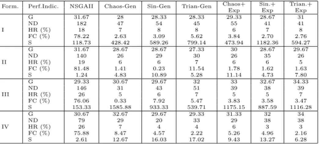
G 31.67 28 28.33 28.33 29.33 28.67 31 ND 182 47 54 45 55 41 41 I HR (%) 18 7 8 8 6 7 8 FC (%) 78.22 2.63 3.09 5.62 3.84 2.70 2.76 S 118.73 428.42 589.26 799.14 473.94 1182.36 594.27 G 31.67 28.67 28.67 27.33 30 28.67 29.67 ND 140 26 29 30 26 35 26 II HR (%) 19 6 6 7 6 6 5 FC (%) 81.48 1.41 0.23 11.54 1.78 1.62 1.63 S 1.24 4.83 10.89 5.28 11.14 4.73 7.80 G 29.33 30.67 29.67 32 33 32.67 34.33 ND 146 31 43 51 39 38 39 III HR (%) 26 5 6 7 5 5 7 FC (%) 76.06 0.33 7.92 5.47 3.83 3.58 3.47 S 153.33 1585.88 933.33 539.71 1175.15 887.59 1116.28 G 30.67 32.67 29.67 29.33 31.33 32 34 ND 79 29 20 33 29 38 38 IV HR (%) 26 7 4 4 6 3 3 FC (%) 75.88 8.47 4.57 2.22 5.26 4.96 2.16 S 2.61 12.67 16.03 17.02 9.43 13.27 6.28