Data assimilation in a multi-scale model

Data assimilation in a multi-scale model

Article

Published Version

Creative Commons: Attribution-Noncommercial-No Derivative Works 4.0

Open Access

Hu, G. and Franzke, C. L. E. (2017) Data assimilation in a

multi-scale model. Mathematics of Climate and Weather

Forecasting, 3 (1). pp. 118-139. ISSN 2353-6438 doi:

https://doi.org/10.1515/mcwf-2017-0006 Available at

http://centaur.reading.ac.uk/89879/

It is advisable to refer to the publisher’s version if you intend to cite from the

work. See

Guidance on citing

.

To link to this article DOI: http://dx.doi.org/10.1515/mcwf-2017-0006

Publisher: De Gruyter

All outputs in CentAUR are protected by Intellectual Property Rights law,

including copyright law. Copyright and IPR is retained by the creators or other

copyright holders. Terms and conditions for use of this material are defined in

the

End User Agreement

.

Central Archive at the University of Reading

Reading’s research outputs online

Open Access. © 2017 Guannan Hu and Christian L. E. Franzke, published by De Gruyter Open. This work is licensed under the Creative Commons Attribution-Non-Commercial-NoDerivs 4.0 License.

Research Article

Open Access

Guannan Hu* and Christian L. E. Franzke

Data Assimilation in a Multi-Scale Model

Received June 28, 2017; accepted December 23, 2017

Abstract:Data assimilation for multi-scale models is an important contemporary research topic. Especially the role of unresolved scales and model error in data assimilation needs to be systematically addressed. Here we examine these issues using the Ensemble Kalman filter (EnKF) with the two-level Lorenz-96 model as a conceptual prototype model of the multi-scale climate system. We use stochastic parameterization schemes to mitigate the model errors from the unresolved scales. Our results indicate that a third-order autoregressive process performs better than a first-order autoregressive process in the stochastic parameterization schemes, especially for the system with a large time-scale separation. Model errors can also arise from imprecise model parameters. We find that the accuracy of the analysis (an optimal estimate of a model state) is linearly cor-related to the forcing error in the Lorenz-96 model. Furthermore, we propose novel observation strategies to deal with the fact that the dimension of the observations is much smaller than the model states. We also propose a new analog method to increase the size of the ensemble when its size is too small.

1 Introduction

Forecasting the state of the atmosphere, ocean or climate system requires a numerical model that computes the time evolution of the system, on the one hand, and an estimate for the current state which is used to ini-tialize the model, on the other hand. While the number of observations of the atmosphere and ocean are ever more increasing, we currently still observe the states of the atmosphere and ocean only partially [36].

The uncertainty of predictions is mainly created by two factors: model error and the uncertainty in the ini-tial conditions. Model error is the imperfect representation of the actual system dynamics in a model, which comes from various sources, such as: incomplete dynamics in the numerical model, imprecise knowledge of model parameters in the governing equations, unresolved small-scale processes and numerical approxi-mations, among others [29]. These drawbacks of the model cannot be eliminated because of limited intellec-tual and computational resources; all discrepancies between a numerical model and the acintellec-tual system are not necessarily known. The uncertainty in the initial conditions is an additional factor preventing us from achieving skillful forecasts. With advanced techniques, the state of a system can be measured with high pre-cision. But in real world applications, some direct measurements of a system state are not feasible and the observations typically have a much lower resolution in space and time compared to the numerical models. Therefore, the observations are not sufficient to initialize the numerical models and we need to use all useful available observations to estimate initial values of all model variables. Data assimilation is such a method which extracts information from observations and model forecasts and provides improved state estimates of relevant variables and reconstructs the 3-dimensional state variables [13]. Data assimilation is widely applied to atmospheric and oceanic systems [13, 25, 36] and also extended to the coupled climate system for seasonal forecasts.

*Corresponding Author: Guannan Hu:_{School of Integrated Climate System Science, University of Hamburg, Hamburg,}

Ger-many

and Meteorological Institute, University of Hamburg, Hamburg, Germany

and Center for Earth System Research and Sustainability, University of Hamburg, Hamburg, Germany, E-mail: guannan.hu@studium.uni-hamburg.de

Christian L. E. Franzke:Meteorological Institute, University of Hamburg, Hamburg, Germany

One efficient data assimilation scheme is the ensemble Kalman filter (EnKF) proposed in [17]. It has been applied in a number of different contexts [19], and its skill is examined with the applications to various mod-els, from ocean models [14, 30, 38] to atmospheric models [46, 60], from conceptual climate models [18] to global general circulation models [52]. The performance of the EnKF can be limited by an insufficient ensem-ble size and sparse observations. A small number of the ensemensem-ble members can introduce sampling errors and potentially the forecast error covariance is incorrectly estimated. Covariance inflation and localization are two common methods which are used to correct the error covariance [2, 3, 24, 28, 31]. Grooms et al. [27] pointed out that stochastic subgrid-scale parameterizations have the same effect as the covariance inflation techniques, because they increase the ensemble spread. Moreover, instead of using the ensemble evolved from the past analyzed ensemble states, Tardif et al. [58] used the ensemble formed by randomly drawing model states from preexisting integrations to estimate the background error covariance.

An important problem in contemporary climate science is the assimilation of observations into opera-tional coupled seasonal and decadal prediction models. The climate system can be seen, to first order, as a system with two time scales: the slow ocean and the fast atmosphere. The two-level Lorenz-96 model pro-posed in [42] is an ideal testbed for numerical experiments considering the computational requirements, pos-sibility for defining the truth and the chaotic, strongly nonlinear nature [18, 44, 45]. Hence, the results can potentially be seamlessly extended to realistic applications with sophisticated and comprehensive models [8, 45]. The Lorenz-96 system contains coupled equations in two sets of variables. By appropriately choos-ing the parameter values, we can set the time-scale separation between the two sets of variables and test the sensitivity of data assimilation on different time-scale separations. A major challenge in data assimila-tion is the presence of model error [29]. To address this issue, we define two kinds of imperfect models in our numerical experiments. They contain the model errors from the imprecise forcing values and unresolved processes, respectively. Instead of resolving small-scale variables in the Lorenz-96 model, we use stochastic parameterization schemes to represent the influence of the unresolved processes on the resolved large-scale variables. The stochastic parameterization schemes are able to mitigate the model errors due to unresolved scales [5, 29, 50, 53, 54]. A perfect model is used to compare with the imperfect models. The perfect model has a specified forcing value which is considered as the true value and resolves the small-scale variables.

The outline of the paper is as follows: In the next section, the two-level Lorenz-96 model is discussed. We will discuss the time-scale separations, imprecise forcing values and stochastic parameterization schemes for the unresolved small-scale variables. In Sec. 3, brief introductions of data assimilation and the EnKF al-gorithm are presented. We carry out numerical experiments of data assimilation and give the results in Sec. 4. Finally, we end the paper with a discussion and draw a conclusion from our results.

2 The Lorenz-96 System

We reformulate the two-level Lorenz-96 model [42, 45] in such a way that it explicitly contains a parameterε determining the time-scale separation between the two sets of variables of the coupled equations [11, 20]:

dX_k dt = −Xk−1(Xk−2−Xk+1) −Xk+F− h J J X j=1 Y_j,k, (1a) dYj,k dt = 1 ε(−Yj+1,k(Yj+2,k−Yj−1,k) −Yj,k+hXk). (1b)

The large-scaleXkvariables and small-scaleYj,kvariables are defined fork= 1,. . .,Kandj= 1,. . .,J. Each large-scale variable containsJsubgrid-scale variables. In our computations, we set the parameters as follows:K= 18,J= 20, coupling coefficienth= 1.0, and forcingF= 10 as standard values. The parameterε determines the time-scale separation between theXkandYj,kvariables. Forε= 1.0, theXkandYj,kvariables

have the same time scale. Forε < 1.0, theXkvariables have a larger time scale than theYj,kvariables. The smaller the value ofε, the larger the time-scale separation. We can also describe theXkvariables as slow

term [20]: the sum over the fast variables in Eq. (1a).

We list the statistical information of theXkandYj,kvariables of the Lorenz-96 model with different

time-scale separations in Table. 1. AllXkandYj,kvariables have identical statistical properties, respectively. The statistics are calculated from a long-term integration of the Lorenz-96 model with a integration time step

dt = 0.001. The values of time-scale separation are chosen asε = 0.125,ε = 0.25,ε = 0.5 andε = 1.0. Generally, a greater variation of the statistics of theYj,kvariables compared to theXkvariables are found. As

the time-scale separation increases, the maximum and standard deviation of theYj,kvariables become larger, while the minimum and mean decrease. BothXkandYj,kvariables are approximately Gaussian distributed.

A change of the time-scale separation does not alter the distribution.

Table 1:The maximums, minimums, means, and standard deviations of theXkandYj,kvariables in the Lorenz-96 model with

different time-scale separations (ε).

X_k Y_j,k

ε Max Min Mean Sd Max Min Mean Sd

0.125 13.72 −7.33 2.63 3.57 17.58 −13.50 1.03 2.37

0.25 13.59 −7.25 2.53 3.51 17.50 −12.22 1.04 2.35

0.5 13.33 −7.35 2.45 3.54 16.17 −11.50 1.15 2.16

1.0 13.18 −9.04 2.45 3.67 12.91 −10.26 1.25 1.87

2.1 Imprecise Forcing

In a dynamical system which is highly sensitive to the initial conditions, small initial perturbations will lead to widely diverging outcomes. Hence, the medium-term behavior of the system is unpredictable, while the long-term behavior will be determined by the attractor. This behavior is known as deterministic chaos.

The behavior of the Lorenz-96 system is largely determined by the forcingF; the value ofFdetermines the presence or absence of chaos, or appearance of other behaviors [20, 42–45]. For a very small value of

F, all trajectories of the Lorenz-96 system will converge to a steady state, and allXkandYj,kvariables will have an identical value. When the value ofFbecomes somewhat larger, the steady state solution turns into flow regimes where most solutions are periodic or quasi-periodic, but still not chaotic. When the value ofFis large enough (the exact value depends on the dimension of theXkvariables), chaotic flows emerge. The three

different behaviors of the Lorenz-96 system are illustrated in Fig. 1. The time series of the first component of theXkvariables are presented after transients. We observe cyclic behaviors on two time scales whenF= 2.

We calculate the maximal Lyapunov exponent (MLE) of the system. The numerical estimates of them are −1.57, 0.0002 and 7.83 forF= 1,F= 2 andF= 10, respectively.aThe MLE describes the predictability of a dynamical system. Generally, a strictly positive MLE indicates exponential instability and is often considered a signature of deterministic chaos, and a strictly negative MLE indicates stability.

2.2 Unresolved Processes and Parameterizations

Regarding many practical applications, we are only interested in predictions of atmospheric processes on a particular scale rather than the detailed evolution of quantities at smaller scales. In this situation, small-scale processes are not necessary to be resolved and in practice, some predictions are impractical to be resolved due

0.3 0.4 0.5 0.6 0.7

(a)

(b)

Model time unit

0

2

4

6

8

10

12

14

16

18

20

(c)

Figure 1:Time series of theX₁variable in the Lorenz-96 model with the forcing values (a)F= 1, (b)F= 2and (c)F= 10. The time-scale separation isε_{= 0.125}.

to computational restrictions. The impacts of these unresolved processes on the evolution of large-scale pro-cesses can be represented to some degree by suitable deterministic or stochastic terms [4, 23]. This approach is aimed to obtain a reduced model that involves only the variables of interest. To derive reduced versions of the Lorenz-96 model, we use the parameterization schemes introduced in [65], the key idea in which is to use a polynomial equation and a noise term that represent the model error when only theXk variables are resolved in place of the full dynamics. The polynomial equation with noise is written as follows:

P(Xk) =a0+a1Xk+a2X2k+a3X3k+ek(t). (2)

It is used to replace the last term in Eq. (1a). TheXkvariables used in Eqs. (2), (5) and (6) are on time step

tand for concision, the time index is omitted. Eq. (2) mainly depends on the resolvedXkvariables and it is based on the notion that the large scales determine the properties of the unresolved subgrid scales [8]. The cubic form of the parameterization is consistent with stochastic climate theory [22, 23, 26, 47–49]. The cubic

term can be viewed as a nonlinear damping. The coefficients{a0,a1,a2,a3}are determined by fitting a time series of the residuals by a standard least squares method. The time series of the residuals is obtained by taking the difference between the tendency of the full dynamics and reduced tendency with a short time step

δt= 0.005: P(Xk(t)) ≈ X_k(t+δt) −Xk(t) δt − (−Xk−1(t)(Xk−2(t) −Xk+1(t)) −Xk(t) +F). (3)

The first four terms of the right-hand side of Eq. (2) are deterministic and the noise termek(t) is the residual

from the polynomial fitting. If we setek(t) = 0, then we obtain a deterministic parameterization scheme for

the unresolvedYj,kvariables. Ifek(t) are further fitted by an autoregressive process, then we get a stochastic

parameterization scheme. The autoregressive process has the form:

e_k(t) =ϕ1ek(t−δt) +ϕ2ek(t− 2δt) + · · · +ϕpek(t−pδt) +η(t), (4)

where the parameterpdenotes the order of the autoregressive process and determines the memory depth of the time series of the residuals. Theη(t) are Gaussian noise variables with mean zero and varianceσ. The coefficients{ϕi,i= 1, · · · ,p}and the noise varianceσare estimated by the Yule-Walker equations [61, 66]. In addition to a first-order autoregressive process, denoted as AR(1) process, which is considered in [65], we also consider an autoregressive process of order 3, denoted as AR(3) process, in our experiments. This is motivated by the fact that the model reduction introduces memory into the reduced system [26] and should be explicitly modeled.

In summary, we have used polynomial equations and autoregressive processes to represent the variability of the unresolvedYj,kvariables, and the entire governing equations of two reduced versions of the Lorenz-96

model are given as

dX_k dt = −Xk−1(Xk−2−Xk+1) −Xk+F−a0−a1Xk−a2X2k−a3X3k −ϕek(t−δt) −η(t), (5) and dX_k dt = −Xk−1(Xk−2−Xk+1) −Xk+F−a0−a1Xk−a2X2k−a3X3k −ϕ₁ek(t−δt) −ϕ2ek(t− 2δt) −ϕ3ek(t− 3δt) −η(t), (6)

wheredt = δt = 0.005. The reduced models contain two parts: the tendency of the Xkvariables and the

stochastic parameterizations of theYj,kvariables. Here, we call the model described by Eq. (5) the L96-AR1

and Eq. (6) the L96-AR3. In comparison to them, we call Eqs. (1a) and (1b) the full dynamic model (FDM). Parameter values of the L96-AR1 and L96-AR3 are listed in Table. 2. The noise varianceσin the L96-AR3 is one or two order of magnitude lower than in the L96-AR1. Note that the estimated parameter values for eachXk

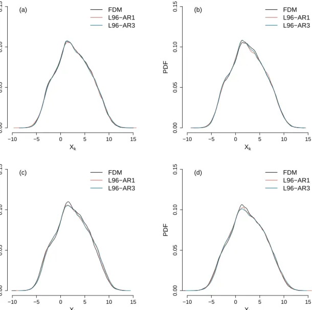
variable are slightly different. We show the mean values of them in the table and use the corresponding values for eachXkvariable in the numerical experiments. We compare the probability density functions (PDF) of the

Table 2:Parameter values of the L96-AR1 and L96-AR3.

Polynomial terms AR(1) process AR(3) process

ε a₀ a₁ a₂ a₃ ϕ σ ϕ₁ ϕ₂ ϕ₃ σ

0.125 0.18 0.42 −0.002 −0.0015 0.9932 0.0031 2.73 −2.58 0.85 9.6e−05

0.25 0.15 0.37 0.008 −0.0019 0.9983 0.0013 2.69 −2.41 0.72 1.7e−05

0.5 0.35 0.22 0.025 −0.0017 0.9994 0.0009 1.92 −0.84 −0.08 1.8e−05

1.0 0.72 0.09 0.022 −0.0011 0.9997 0.0005 1.73 −0.47 −0.26 1.4e−05

and the reduced models are withdt = 0.005. For all values of the time-scale separation, there are small discrepancies between the FDM and reduced models, and they are smaller when the time-scale separation is larger. Fig. 3 presents the autocorrelation functions (ACF) of theXkvariables in the three models. Similar to the comparison of the PDFs, the reduced models well reproduce the ACF of the FDM. Differences are only found in the oscillation of the ACF, especially for the smaller time-scale separations. The AR1 and L96-AR3 are able to capture the features of theXkvariables in the FDM. The model errors of the reduced models

are smaller when the time-scale separation is larger.

Xk PDF 0.00 0.05 0.10 0.15 −10 −5 0 5 10 15 FDM L96−AR1 L96−AR3 (a) Xk PDF 0.00 0.05 0.10 0.15 −10 −5 0 5 10 15 FDM L96−AR1 L96−AR3 (b) Xk PDF 0.00 0.05 0.10 0.15 −10 −5 0 5 10 15 FDM L96−AR1 L96−AR3 (c) Xk PDF 0.00 0.05 0.10 0.15 −10 −5 0 5 10 15 FDM L96−AR1 L96−AR3 (d)

Figure 2:Probability density functions of theXkvariables in three models with the time-scale separations (a)ε = 0.125, (b)

model time unit A CF 0 2 4 6 8 10 −0.5 0.0 0.5 1.0 1.5 _FDM L96−AR1 L96−AR3 (a)

model time unit

A CF 0 2 4 6 8 10 −0.5 0.0 0.5 1.0 1.5 _FDM L96−AR1 L96−AR3 (b)

model time unit

A CF 0 2 4 6 8 10 −0.5 0.0 0.5 1.0 1.5 _FDM L96−AR1 L96−AR3 (c)

model time unit

A CF 0 2 4 6 8 10 −0.5 0.0 0.5 1.0 1.5 _FDM L96−AR1 L96−AR3 (d)

Figure 3:Autocorrelation functions of theXkvariables in three models with the time-scale separations (a)ε = 0.125, (b)ε =

0.25, (c)ε= 0.5and (d)ε= 1.0.

3 Data Assimilation

Data assimilation is the combination of the information from observational data and a numerical model forecast. Data assimilation schemes can be roughly divided into two categories: ensemble-based methods [1, 17, 19, 31, 32, 64] and variational methods [10, 39, 40, 56]. Variational methods such as three-dimensional or four-dimensional variational data assimilation (3D-Var or 4D-Var) rely on tangent linear operators and adjoint equations. Ensemble-based data assimilation techniques include the ensemble Kalman filter (EnKF), ensemble Kalman smoother (EnKS) and ensemble transform Kalman filter (ETKF), which all depend on statis-tical estimates from ensemble forecasts. Most pracstatis-tical ensemble-based data assimilation schemes are some kind of approximations of the celebrated Kalman filter [34, 35]. All of them are aimed to either reduce the computing requirements or to improve the statistical forecasts, or both. The EnKF is an efficient ensemble-based data assimilation scheme [16, 17, 19]. This Monte Carlo approximation of the Kalman filter efficiently reduces the computational requirements and directly provides initial perturbations for ensemble forecasts. The main disadvantages of the EnKF are that an insufficient ensemble size and sparse observations limit the

quality of the produced analysis fields. These shortcomings of the EnKF contrast the advantages of 4D-Var, which produces useful analysis even when observations are sparse and do not need ensembles. The disad-vantages of 4D-Var include the developing and maintenance of tangent linear and adjoint models and that many physical parameterization schemes contain step functions. If the assimilation window for 4D-Var is too short, the EnKF performs better than 4D-Var, while for infrequent observations 4D-Var gives more accurate estimates [15, 21, 33, 37, 40, 63]. In practice, hybrid approaches are often adopted [6, 7, 9, 62]. In this paper we use the EnKF.

3.1 The Ensemble Kalman Filter

Here, we briefly introduce the algorithm of the EnKF. Comprehensive theoretical aspects and the numerical implementation are provided in [19]. There are two stages involved in a sequential data assimilation method-ology: (i) the forecast and (ii) the update stage. During the forecast stage, we use a, possibly nonlinear, model to forecast the system state of dimensionn,ψft ∈Rnand the error covariance of the model forecast,P

f

t ∈Rn×n,

wherefdenotes forecast andtis the time index. When we assimilate observations to theXkvariables in the

FDM and reduced models,ψft represents theXkvariables andn = K. When we assimilate observations to theYj,kvariables in the FDM,ψft represents theYj,kvariables andn=KJ. In a deterministic model,ψft only

depends on the former stateψft−1.P

f

tis defined in terms of the true stateψ ref t as: Pf_t = (ψft −ψ ref t )(ψ f t −ψ ref t )T, (7)

where the overbar denotes an expectation value andTmeans the transpose of a matrix. The true state is un-known and different algorithms are used to estimatePft. For a linear model, the evolution equation is written

in discrete form as:

ψf_t =Ftψat−1+wt, (8)

whereFtis a transition matrix,adenotes analysis which is obtained in the update stage, andwtis a Gaus-sian noise vector with zero mean, representing the model error. The evolution equation of the forecast error covariance becomes

Pf_t =FtPat−1F

T

t +Qt, (9)

whereQtis the error covariance matrix for the model errorwt. With a nonlinear model written as:

ψf_t =ft(ψat−1) +wt, (10)

whereftis the forecast operator, the evolution equation of the forecast error covariance is the same as Eq. (9), but withFtbeing the tangent linear operator offt. In the EnKF, the forecast error covariance is computed by Eq. (7), using the ensemble meanψft to replace the unknown true stateψ

ref

t [19]. Considering an ensemble

of model forecasts with a size ofN, Eq. (7) becomes

Pf_t = _N1 − 1 N X i=1 (ψft,i−ψ f t)(ψ f,i t −ψ f t) T . (11)

The second stage in a sequential data assimilation methodology is the update stage, or analysis step. The update stage takes place when the observationsd∈Rmof a system state are available. We neglect the time indextof this stage, because all vectors and matrices in this stage are at the same time step. Observations usually have a smaller dimension compared to the model state,m6n. The observation data may also need to be transformed in order to fit the model output. Therefore, a linear measurement operatorH ∈ Rm×nis used, which relates the true state to the observations

d=Hψref +ϵ, (12)

whereϵis measurement errors.H∈Rm×nmaps the model state inRnto the observation space inRm. Now we have both observations and model forecasts of a system state, and we can use them to estimate the true

state. The estimated system state is called analysisψain data assimilation. The analysis is determined as a weighted linear combination of forecasts and observations:

ψa=ψf+K(d−Hψf), (13)

whereK∈Rn×mis called the Kalman gain matrix, which is determined by the error covariance of the forecasts and observations:

K=PfHT(HPfHT+R)−1, (14)

whereR∈Rm×mis the error covariance matrix for the observations and defined as

R=ϵϵT. (15)

The error covariance of the forecast is also called background error covariance in the update stage. The error covariance of the analysis is obtained by updating the background error covariance:

Pa= (I−KH)Pf. (16)

Eqs. (13), (14) and (16) are the equations of the standard Kalman filter in the update stage. In the EnKF, the computation of the error covariance of the analysis is not required, because at each analysis step, the back-ground error covariance used in Eq. (14) is directly calculated by Eq. (11) instead of using Eq. (9) to evolvePa. In addition, an ensemble of observations is defined as:

di=d+ϵi, i= 1, . . . ,N, (17)

whereϵiare Gaussian noise variables with zero mean and prescribed variance. The error covariance of the observations becomes R= _N1 − 1 N X i=1 (di−d)(di−d)T. (18)

As described above, the analysisψaand the error covariance of the analysisPaare computed during the update stage. They are used to initialize the Eqs. (8) and (9) for linear models and the Eqs. (9) and (10) for nonlinear models in the prediction stage, then the model state and the error covariance are integrated for-ward in time. Whenever observations are available, the update stage takes place and the analysis and error covariance of the analysis are calculated and used again to initialize the model in the next prediction stage. In the EnKF, the evolution and update of the error covariance of the forecast are not required.

4 Numerical Data Assimilation Experiments

In this section, we perform the EnKF with the FDM, L96-AR1 and L96-AR3. We will first describe the experi-mental settings and the performance measures of the EnKF we use. Next, we will show the influence of the ensemble size on the performance of the EnKF and give a method to inflate an ensemble which has an insuf-ficient size. Then, we will discuss how the distribution of observations affects the performance of the EnKF and give observation strategy. Finally, we compare the imperfect models, in which model errors come from the imprecise parameters and unresolved processes.

4.1 Experimental Setup

As described in Sec. 3.1, in order to implement the ensemble Kalman filter (EnKF), a forecast model and ob-servation data are needed. In our numerical experiments, we use the FDM, L96-AR1 and L96-AR3 described in Sec. 2 to generate ensemble forecasts. Observations are created by addingϵ∼N(0, 0.1) to the true states

generated by the FDM with standard forcing value. Our results are not sensitive to the exact value of the ob-servation noise. To generate truth, the FDM is integrated using a fourth-order Runge-Kutta scheme, with a time step ofdt= 0.001. The initial values are randomly sampled from a Gaussian distribution and we take the true trajectory after a transient.

The maximal Lyapunov exponent (λmax) of the FDM proportionally increases with an increase of the time-scale separation. We getλmax ≈ 7.83 for the time-scale separationε = 0.125. Using the equation given by

E(t) = E0e

λmaxt

1 +E0(eλmaxt− 1)

(19) we can estimate the doubling time of small errors in initial conditions [36, 41]. The doubling time is the pe-riod of time over which the magnitude of a quantity will double.Erepresents the root-mean-square average forecast error and it is scaled so that at long forecast leadsE→1.E0is the initial error and grows toE(t) by timet. For a initial errorE0= 0.02 and aλmaxof value 7.83, the doubling time is about 0.09 model time unit (MTU). The value of the initial error is the averaged analysis error of the FDM. In practice, small initial errors in synoptic scales double in about 2 days [12, 57, 59] and the data assimilation window lengths are 3h, 6h or 12h. If we calibrate the interval between two analysis steps in our experiments to the assimilation window in practice via the doubling time, then the interval is too short and the EnKF will diverge. Therefore, we choose the error doubling time 0.09 MTU as the analysis interval.

In our experiments, the analysis and forecast errors are measured in terms of root-mean-square error (RMSE), which is used as the performance measure of the EnKF. The error is defined as the difference be-tween the analysis (forecast) and true state of the control simulation. The equation for calculating the RMSE is given as RMSE= v u u t 1 KN N X i=1 K X k=1 (X_ka(f),i−Xctrl_k )2_{, (20)}

wherekcounts for each state variable andifor each ensemble member. We only calculate the RMSE of the

Xkvariables in order to make fair comparison between the FDM and reduced models. Unlike the control sim-ulation (generation of the truth), model forecasts are produced by using a fourth-order Runge-Kutta scheme, with a time stepdt= 0.005 (MTU). We implement the EnKF every 18 time steps (analysis intervaldt= 0.09) in 10-MTU simulations, which means 111 analysis steps in each simulation. The EnKF converges during the first several analysis steps and after it has converged, we generate 10-MTU forecasts from the desired initial conditions provided at the analysis steps. We calculate the RMSE of theXkvariables at each analysis step

and each integration time step in forecasts. We use plots of the mean and standard deviation and box plots to present the values of the RMSE of the analysis. We average the values of the RMSE over the same integration time steps in forecasts and show the averaged RMSE value as a function of forecast lead time.

We apply the same observation errors and observe the same subset of variables for all three models. In Secs. 4.2, 4.4 and 4.5, we observe allXkvariables. In Sec. 4.3, we observe theXkvariables, theXkandYj,k vari-ables and other 4 different subsets of varivari-ables. We choose ensemble sizeN= 100 for the reduced models and the FDM when only theXkvariables are observed. If we also assimilate observations to theYj,kvariables in the FDM, then we need a larger ensemble size, which isN= 2000, and also a larger analysis interval, which isdt = 0.27, to prevent the divergence of the EnKF. The figures in Sec. 4 show the results of the time-scale separationε= 0.125, when we do not give the time-scale separation in the captions.

4.2 Ensemble Size

When we apply the EnKF, a proper size of the ensemble has to be chosen. On the one hand, the ensemble size has to be large enough in order to reduce the sampling error which causes the inaccurate estimation of the error covariance of the forecasts. This influences the performance of the EnKF. On the other hand, we need to avoid a too large number of ensemble members which requires and takes up a lot of computing resources. The performance of the EnKF reaches a plateau for a certain ensemble size, beyond this ensemble size the

improvement in the performance is very small. It is possible to use thousands or even more ensemble mem-bers for the Lorenz-96 system in our numerical experiments and we could demonstrate this saturation effect. However, this is impossible for seasonal prediction systems, which only use on the order of 10 to 60 ensemble members.

To estimate a proper ensemble size for our numerical experiments, we implement the EnKF in three

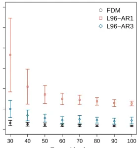
mod-● _● ● ● ● ● ● ● 0.00 0.05 0.10 0.15 0.20 0.25 0.30 Ensemble size RMSE of analysis 30 40 50 60 70 80 90 100 ● _FDM L96−AR1 L96−AR3

Figure 4:Means and standard deviations of the RMSE of the analysis for different sizes of the ensemble.

els with the ensemble size changing from 30 to 100 with interval 10. Fig. 4 shows the means and standard deviations of RMSE of the analysis for different ensemble sizes. The RMSE of the analysis is larger for the smaller ensembles, especially in the reduced models, and decreases rapidly with an increase in ensemble size, but it cannot drop to zero because of observational noise, imperfection of the model, and the represen-tation of the truth by the ensemble mean. The analysis error of the L96-AR1 reaches to a plateau when the ensemble size is aboutN= 100, which is greater than the ensemble sizes the FDM and L96-AR3 need.

Using Monte Carlo simulations to obtain the background error covariance is an efficient modification of the extended Kalman filter (EKF) in the EnKF [18, 51, 55]. It reduces the computational demands in the nonlin-ear dynamical system (e.g., the computation of the tangent linnonlin-ear operator). However, for large models it also becomes expensive due to the requirement of a sufficient number of ensemble members. An insufficient en-semble size will introduce sampling error and lead to wrong estimates of the background error covariance. We can use some methods to increase the sample size. For instance, we can draw model states from preexisting integrations to form ensembles [58]. However, if these model states are randomly drawn, they will increase the background errors. Therefore, we use observations to find so-called analogs in the model states and use them as additional ensemble members. We define the analogs as the model states which have small values of the root-mean-square deviation to the observations. The values should be smaller than a prescribed thresh-old. However, if we set the threshold too low, no or only a small amount of analogs can be found and they only slightly improve the performance of the EnKF. If the threshold is too high, the analogs bring too much error which makes the skill of the EnKF worse. To overcome this problem, we only pick the analog which is closest to the observations at each analysis step, and duplicate it many times to form the ensemble with the desired size. For instance, we duplicate the analog 10 times, and use them with 10 regular ensemble members to form a 10 + 10-member regular + analog ensemble. The analogs are only used to estimate the background error covariance and not integrated in the prediction stage to make forecasts. We compare a 10-member

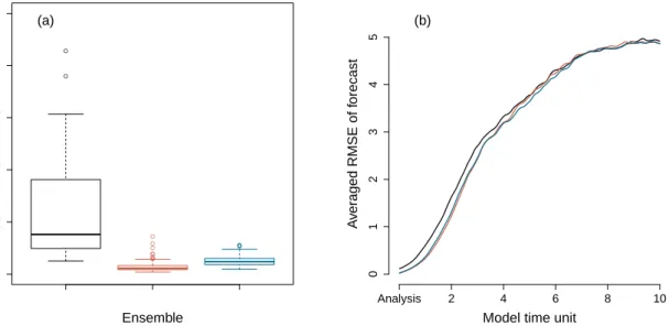
reg-ular ensemble, a 10 + 10-member regreg-ular + analog ensemble, and a 20-member regreg-ular ensemble in Fig. 5. We only calculate the analysis and forecast errors of the 10 regular ensemble members in the 10 + 10-member ensemble. The results show that using analogs to inflate an insufficient ensemble greatly improves the anal-ysis and forecast of the regular ensemble members. Moreover, even for the ensembles with the same size, the EnKF slightly performs better when using analogs to replace part of the regular ensemble members. This is because the analogs have smaller errors than the regular ensemble members in the experiments of the FDM. We may also think of using analogs instead of analysis as the initial conditions. However, the averaged RMSE value of the analogs is greater than the averaged RMSE value of the analysis obtained by using the analogs. In some cases, even though the analogs have larger errors than the regular ensemble members and actually increase the background error, using them to inflate an insufficient ensemble still improves the accuracy of the analysis and forecast. This is found in the experiments of the reduced models (not shown).

● ● ● ● ● ● ● ● ● ● ● ● ● ● 0.0 0.1 0.2 0.3 0.4 0.5 Ensemble RMSE of analysis (a)

Model time unit

A v er aged RMSE of f orecast 0 1 2 3 4 5 Analysis 2 4 6 8 10 (b)

Figure 5:(a) Box plots of the RMSE of the analysis and (b) averaged RMSE of the forecasts as a function of forecast lead time of the FDM. Black: 10-member regular ensemble. Red: 10 + 10-member regular + analog ensemble. Blue: 20-member regular ensemble.

4.3 Observation Strategy

In the Lorenz-96 model, the large-scale variablesXkare coupled to many small-scale variablesYj,k, and they

dominate the activity of theYj,kvariables. If theXkvariables have large positive values, then the

correspond-ingYj,kvariables, those with the samekvalues, become active, otherwise they evolve with a small amplitude

in time [42]. Unlike this great effect of theXkvariables on theYj,kvariables, the impact of theYj,kvariables

on theXkvariables is much smaller. When we use the reduced models to produce forecasts, we can only

as-similate observations to theXk variables, since theYj,kvariables are not resolved any longer. When using

the FDM, we also resolve theYj,kvariables. If we need to predict theYj,kvariables, it is necessary that both

X_kandYj,kvariables are assimilated with observations. If we are only interested in the forecasts of theXk

variables, the question arises, whether we should assimilate observations to theYj,kvariables and how large

its influence is on the forecasts of theXkvariables. There are many moreYj,kthanXkvariables. Therefore, we

would need many more ensemble members to estimate the background error covariance when we assimilate observations to theYj,kvariables. This is time consuming and, thus, undesirable.

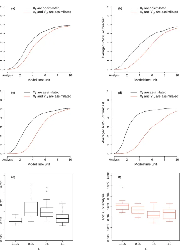
of theXkvariables for different values of the time-scale separation. We present the averaged RMSE of the forecasts as a function of forecast lead time, as well as the box plots of the RMSE of the analysis. TheYj,k

variables are not modified at the analysis steps when we only assimilate observations to theXk variables. When the time-scale separation is larger, the difference of the forecasts between assimilating and not assimi-lating observations to theYj,kvariables is smaller. There is a trade-off between the effort of observing theYj,k variables and assimilating observations to them and the accuracy of the forecasts of theXkvariables. Clearly,

the effort is independent of the time-scale separation while the improvement of the forecasts becomes less as the time-scale separation increases. This suggests that we can consider assimilating only slow variables in a system with a large time-scale separation.

In our numerical experiments, we can simply generate observations of every variable. But in real world predictions, the dimension of available observations is much smaller than the number of model variables. Therefore, we choosem= 9, half of the number of theXkvariables, as the dimension of the observations for

the models. TheXkvariables can be thought of as values of some atmospheric quantity discretized atKgrid points and we can only measure half of them. Imagine that we use Argo floats to measure the temperature and salinity of the ocean and need to consider the changing positions of the Argo floats. For the given observa-tion dimension, there are many different subsets of theXkvariables which are observed. Using the equation

C(K,m) = _(K−K_m!_)!m!, we get the number of 9-combinations of 18 which is 48620. The number of the combina-tions is too large for us to compare all of them. We consider four cases of observed variables: 1) allXkvariables

are observed; 2) half of theXkvariables with continuous values ofkare observed, i.e.X1,X2, . . . ,X9; 3) ev-ery other of theXkvariables are observed, i.e.X1,X3, . . . ,X17; and 4) first halfXkvariables are observed

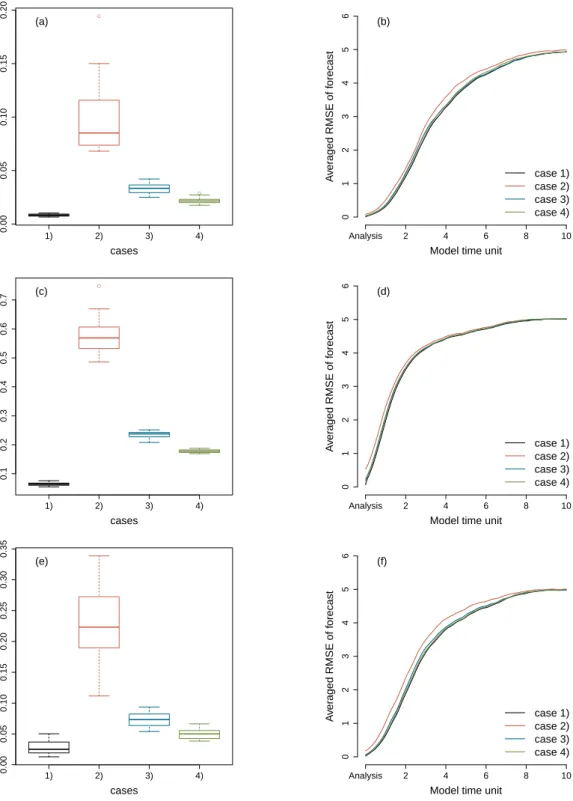
at the first (odd) analysis step, i.e.X1,X2, . . . ,X9, then second halfXk variables are observed in the next (even) analysis step, i.e.X10,X11, . . . ,X18. Fig. 7 presents the box plots of the RMSE of the analysis and averaged RMSE of the forecasts as a function of forecast lead time in these four cases. The results in the three models are consistent: case 3) and 4) show the smallest analysis and forecast errors when only half of the

Xkvariables are observed and the EnKF also converges faster in case 3) and 4) (not shown). In the L96-AR1, the analysis error is greater than the observation error in all three cases of observing half of theXkvariables,

while this only happens in case 2) of the L96-AR3. We only show the results when the time-scale separation isε= 0.125, because for all values of time-scale separation considered, consistent results are found.

4.4 Full Dynamic Model with Imprecise Forcing

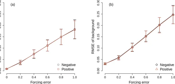
The forcing value in our control simulation isF= 10. Different values ofFwill result in different dynamics of the system. The larger the difference, the greater the change of the dynamics. A too small forcing value will lead to the appearance of different behaviors of the Lorenz-96 system while a too large forcing value will greatly increase the saturation error, which is the maximal forecast error caused by the uncertainty in the initial conditions. We now choose imprecise forcing values from 9 to 11 with interval 0.2, which have the forcing error smaller or equal to 10% of the standard forcing value. We do not want to change the dynamics and reduce the predictive skill of the imprecise models too much. Fig. 8 shows the analysis and background errors of the FDM with different forcing errors. The positive errors mean that the errors are added to the stan-dard forcing value and the negative errors mean subtraction. Although the Lorenz-96 system is chaotic and strongly nonlinear, the RMSE of the analysis linearly increases as the forcing error becomes larger. When the forcing error is greater than 0.6, the analysis error is larger than the observation error. Moreover, the RMSE of the background also has a linear correlation with the forcing error. This is the reason for the linear correlation of the analysis and forcing errors. Because the analysis is obtained by a linear combination of the background and observations (Eq. (13)). There is no obvious difference between the negative and positive errors for the RMSE of the analysis and background. Fig. 9 presents the forecast errors of the FDM with different forcing values as a function of forecast lead time. As the forcing error increases, the forecast error becomes larger. Unlike the analysis error, there is an obvious difference of forecast error between the positive and negative forcing errors: the positive forcing errors lead to faster growths of the forecast errors in the medium-term and long-term predictions and also larger saturation errors. This difference is more obvious when the forcing error

Model time unit A v er aged RMSE of f orecast 0 1 2 3 4 5 6 7 Analysis 2 4 6 8 10 Xk areassimilated

Xk andYj,k areassimilated

(a)

Model time unit

A v er aged RMSE of f orecast 0 1 2 3 4 5 6 7 Analysis 2 4 6 8 10 Xk areassimilated

Xk andYj,k areassimilated

(b)

Model time unit

A v er aged RMSE of f orecast 0 1 2 3 4 5 6 7 Analysis 2 4 6 8 10 Xk areassimilated

Xk andYj,k areassimilated

(c)

Model time unit

A v er aged RMSE of f orecast 0 1 2 3 4 5 6 7 Analysis 2 4 6 8 10 Xk areassimilated

Xk andYj,k areassimilated

(d) ● ● ● 0.125 0.25 0.5 1.0 0.000 0.010 0.020 0.030 ε RMSE of analysis (e) ● 0.125 0.25 0.5 1.0 0.000 0.001 0.002 0.003 0.004 0.005 0.006 ε RMSE of analysis (f)

Figure 6:Averaged RMSE of the forecasts as a function of forecast lead time. The time-scale separations are (a)ε= 0.125, (b)

ε= 0.25, (c)ε= 0.5and (d)ε= 1.0. Box plots of the RMSE of the analysis: (e) AllXkvariables and (f) allXkandYj,kvariables

are assimilated.

is larger. The reason is that the Lorenz-96 model with a larger forcing value is more chaotic, which is revealed by the larger maximal Lyapunov exponent. We only show the figures for the time-scale separationε= 0.125, and for the other three values ofε, the results are consistent.

● ● 1) 2) 3) 4) 0.00 0.05 0.10 0.15 0.20 cases RMSE of analysis (a)

Model time unit

A v er aged RMSE of f orecast 0 1 2 3 4 5 6 Analysis 2 4 6 8 10 case 1) case 2) case 3) case 4) (b) ● 1) 2) 3) 4) 0.1 0.2 0.3 0.4 0.5 0.6 0.7 cases RMSE of analysis (c)

Model time unit

A v er aged RMSE of f orecast 0 1 2 3 4 5 6 Analysis 2 4 6 8 10 case 1) case 2) case 3) case 4) (d) 1) 2) 3) 4) 0.00 0.05 0.10 0.15 0.20 0.25 0.30 0.35 cases RMSE of analysis (e)

Model time unit

A v er aged RMSE of f orecast 0 1 2 3 4 5 6 Analysis 2 4 6 8 10 case 1) case 2) case 3) case 4) (f)

Figure 7:Box plots of the RMSE of the analysis and averaged RMSE of the forecasts as a function of forecast lead time of the FDM (a, b), L96-AR1 (c, d) and L96-AR3 (e, f). Cases 1) - 4) are explained in the main text.

4.5 Reduced Model with Stochastic Parameterization

As described in Sec. 2.2, we have defined two reduced models, the L96-AR1 and L96-AR3, which contain stochastic parameterization schemes including a first-oder autoregressive process and an autoregressive pro-cess of order 3, respectively. The stochastic parametrization schemes mitigate the model errors arising from

● ● ● ● ● ● Forcing error RMSE of analysis 0.00 0.05 0.10 0.15 0.20 0.25 0.30 0 0.2 0.4 0.6 0.8 1.0 ● _Negative Positive (a) Forcing error RMSE of background 0.00 0.05 0.10 0.15 0.20 0.25 0.30 0 0.2 0.4 0.6 0.8 1.0 Negative Positive (b)

Figure 8:Means and standard deviations of the RMSE of the (a) analysis and (b) background of the FDM with different forcing errors.

Model time unit

A v er aged RMSE of f orecast 0 1 2 3 4 5 6 Analysis 2 4 6 8 10 F=9.8 F=9.6 F=9.4 F=9.2 F=9 F=10 F=10.2 F=10.4 F=10.6 F=10.8 F=11

Figure 9:Averaged RMSE of the forecasts of the FDM with different forcing values as a function of forecast lead time.

not resolving theYj,kvariables, but it cannot eliminate the model errors. As shown in Fig. 10, the FDM has

the smallest RMSE of the analysis for all values of the time-scale separation considered. For the time-scale separationsε= 0.125 andε= 0.25, the L96-AR3 has smaller analysis errors than the L96-AR1. This indicates that the memory is essential for a better representation of the effect of the unresolved scales. We list the means and standard deviations of the ensemble spread and RMSE of the background at analysis steps in Table. 3. We can find that the accuracy of the analysis mainly depends on the RMSE of the background; the smaller the RMSE of the background, the smaller the RMSE of the analysis. The L96-AR1 has the largest RMSE of the background for all values of the time-scale separation, and it reduces as the time-scale separation decreases. Compared to the L96-AR1, the L96-AR3 has a smaller RMSE of the background, but it increases with a decrease of the time-scale separation. Besides the RMSE of the background, the ensemble spread also influences the

accuracy of the analysis; the larger the ensemble spread, the smaller the RMSE of the analysis. For time-scale separationsε = 0.5 andε = 1.0, even though the L96-AR3 has a slightly smaller RMSE of the background than the L96-AR1, but it has a worse analysis because of the smaller ensemble spread.

Fig. 11 presents the forecast errors of the three models with different time-scale separations. For all values of the time-scale separation, the forecast error grows slower in the L96-AR3 compared to the L96-AR1. The larger the time-scale separation, the better the predictive skill of the L96-AR3. When there is no time-scale separation (ε= 1.0), the forecast errors of the L96-AR1 and L96-AR3 are close. For the time-scale separations

ε= 0.125 andε= 0.25, the L96-AR3 has the most accurate forecasts which are much better than the L96-AR1. In summary, the L96-AR3 has a better predictive skill when the time-scale separation is larger. On the

● ● ● ● ● ● ● ● FDM L96−AR1 L96−AR3 0.00 0.05 0.10 0.15 Models RMSE of analysis (a) ● ● ● ● ● ● ● ● ● FDM L96−AR1 L96−AR3 0.00 0.05 0.10 0.15 Models RMSE of analysis (b) ● ● ● ● ● ● ● ● FDM L96−AR1 L96−AR3 0.00 0.05 0.10 0.15 Models RMSE of analysis (c) ● ● ● ● ● ● ● ● ● ● ● FDM L96−AR1 L96−AR3 0.00 0.05 0.10 0.15 Models RMSE of analysis (d)

Figure 10:Box plots of the RMSE of the analysis. The time-scale separations are (a)ε= 0.125, (b)ε= 0.25, (c)ε= 0.5and (d)

ε= 1.0.

other hand, the short-term predictive skill of the L96-AR1 drops with an increase of the time-scale separation. The L96-AR3 performs better than the L96-AR1, especially for a system with a large time-scale separation. This suggests that memory effects are important for the reduced Lorenz-96 model.

Model time unit A v er aged RMSE of f orecast 0 1 2 3 4 5 Analysis 2 4 6 8 10 FDM L96−AR1 L96−AR3 (a)

Model time unit

A v er aged RMSE of f orecast 0 1 2 3 4 5 Analysis 2 4 6 8 10 FDM L96−AR1 L96−AR3 (b)

Model time unit

A v er aged RMSE of f orecast 0 1 2 3 4 5 Analysis 2 4 6 8 10 FDM L96−AR1 L96−AR3 (c)

Model time unit

A v er aged RMSE of f orecast 0 1 2 3 4 5 Analysis 2 4 6 8 10 FDM L96−AR1 L96−AR3 (d)

Figure 11:Averaged RMSE of the forecasts as a function of forecast lead time. The time-scale separations are (a)ε= 0.125, (b)

ε= 0.25, (c)ε= 0.5and (d)ε= 1.0.

Table 3:The ensemble spread (ES) and RMSE of the background (RMSE_b) of the three models with different time-scale separa-tions (ε).

FDM L96-AR1 L96-AR3

ε ES RMSE_b ES RMSE_b ES RMSE_b

0.125 0.02 ± 0.002 0.03 ± 0.004 0.24 ± 0.005 0.25 ± 0.005 0.04 ± 0.001 0.06 ± 0.006

0.25 0.03 ± 0.002 0.04 ± 0.005 0.16 ± 0.003 0.17 ± 0.005 0.02 ± 0.001 0.07 ± 0.011

0.5 0.03 ± 0.001 0.04 ± 0.005 0.13 ± 0.003 0.15 ± 0.007 0.02 ± 0.001 0.11 ± 0.032

5 Discussion and Conclusion

We have carried out numerical experiments of data assimilation with a prototype multi-scale model of the climate system. We evaluated the effects of different representations of model error and their sensitivity to-ward time-scale separations. We considered two kinds of model error. The first one is an incorrect parameter setting, by changing the forcing value in the Lorenz-96 model. The forcing value largely determines the be-havior of the Lorenz-96 system. The system becomes chaotic only when the forcing value is large enough. For all forcing values considered in our experiments, the Lorenz-96 model is chaotic. The results show that the increase of the forcing error leads to a linear growth of the analysis error, although the Lorenz-96 model is strongly nonlinear. The analysis error is only affected by the absolute value of the constant-in-time forcing error, while the forecast error is also influenced by the sign of the forcing error. For a pair of positive and negative errors which have the same absolute value, the positive errors cause larger forecast errors than the negative errors. The greater the absolute value of the forcing error, the larger the difference in the forecast errors. This is because, if the forcing value is larger, then the maximal Lyapunov exponent of the Lorenz-96 system is also larger. A larger maximal Lyapunov exponent means that the system is more chaotic and un-predictable.

The second type of model error is from unresolved processes. In order to mitigate this kind of model error, we applied stochastic parameterization schemes to the unresolved processes. The stochastic parame-terization schemes represent the effects of the unresolved processes on the resolved variables. They contain deterministic and stochastic terms. The deterministic term is a cubic polynomial equation and the stochastic term is an autoregressive process. Our results show that an autoregressive process with a higher order im-proves over a first-order autoregressive process in parameterizing the fast dynamics in the Lorenz-96 model. The L96-AR3, which contains an autoregressive process of order 3, has a more accurate analysis and a better predictive skill than the L96-AR1, which contains a first-order autoregressive process. This better performance is more obvious when the time-scale separation is larger. Both the L96-AR1 and L96-AR3 more closely repro-duces the statistic of the FDM when the time-scale separation is larger, while the short-term predictive skill of the L96-AR1 decreases with an increase of the time-scale separation. Overall, our results on the Lorenz-96 model indicate that the modelling of memory effects improves data assimilation performance.

As discussed in Sec. 3, the sparse observations limit the performance of the EnKF. In realistic circum-stances, the dimension of observations is always much lower than the dimension of the model state. There-fore, we want to find out which variables are more useful to be observed for a given dimension of observations. Our results on the Lorenz-96 model indicate that assimilating observations to the fast variables has smaller influence on the forecasts of the slow variables when the time-scale separation between the fast and slow variables is larger. Certainly, we need less observations and a smaller ensemble if we only assimilate obser-vations to the slow variables. Therefore, we can consider not observing the fast variables and not assimilating observations to them for the systems with a large time-scale separation. We also found that the EnKF performs better with the widely distributed observations than with observations concentrated on a region. Moreover, if we observe different subsets of the variables at each analysis step, and make sure all variables are observed in a short observation window, then we can get an accurate analysis which is close to the analysis obtained by observing all variables at one analysis step.

An insufficient size of the ensemble is the other factor which restricts the performance of the EnKF. For large models, a sufficient number of ensemble members is often unaffordable. In the EnKF, the ensembles are used to compute the background error covariance at the analysis steps. To reduce the sampling error caused by a small ensemble, which leads to wrong estimates of the background error covariance, we increase the ensemble size by adding analogs at each analysis step. Our results show that the performance of the EnKF is greatly improved when we add analogs in an ensemble which has an insufficient size. In our experiments, we used a simple method to find the analogs. At each analysis step, we calculated the root-mean-square de-viation of each model state to the observations and chose the model state which has the smallest dede-viation as the analog. Model states were drawn from a preexisting long-term integration. This selection procedure of the analogs can be easily done in the Lorenz-96 model, but in real world prediction system we need a very

large disk space to store the long-term integrations and the selection procedure is much more time consuming because of the larger resolution and number of the model variables.

Acknowledgement: We thank Prof. V. Lucarini, Dr. F. Lunkeit, and V. M. Galfi for helpful discussions. We are grateful for the support of computing Lyapunov exponents by Dr. S. Schubert. We wish to express our great thanks and sincere gratitudes to Dr. T. Bodai and an anonymous reviewer, who gave us valuable inputs and constructive criticisms. GH is funded by the China Scholarship Council (CSC). CF is supported by the German Research Foundation (DFG) through the collaborative research center TRR 181 "Energy Transfers in Atmosphere and Ocean" at the University of Hamburg and DFG Grant FR3515/3-1.

References

[1] J. L. Anderson,An Ensemble Adjustment Kalman Filter for Data Assimilation, Monthly Weather Review, 129 (2001), pp. 2884–2903.

[2] ,An adaptive covariance inflation error correction algorithms for ensemble filters, Tellus, 59 (2007), pp. 210–224. [3] J. L. Anderson and S. Anderson,A Monte Carlo implementation of the nonlinear filtering problem to produce ensemble

assimilations and forecasts, Mon. Weather Rev., 127 (1999), pp. 2741–2758.

[4] J. Berner, U. Achatz, L. Batte, L. Bengtsson, A. d. l. Cámara, H. M. Christensen, M. Colangeli, D. R. Coleman, D. Crom-melin, S. I. Dolaptchiev, et al.,Stochastic parameterization: Toward a new view of weather and climate models, Bulletin of the American Meteorological Society, 98 (2017), pp. 565–588.

[5] T. Berry and J. Harlim,Linear theory for filtering nonlinear multiscale systems with model error, Proc. Roy. Soc. London, 470A (2014).

[6] M. Bonavita, L. Isaksen, and E. Holm,On the use of EDA background error variances in the ECMWF 4D-Var, Quarterly Journal of the Royal Meteorological Society, 138 (2012), pp. 1540–1559.

[7] M. Bonavita, L. Raynaud, and L. Isaksen,Estimating background-error variances in the ECMWF Ensemble of Data Assimila-tions system: some effects of ensemble size and day-to-day variability, Quarterly Journal of the Royal Meteorological Society, 137 (2011), pp. 423–434.

[8] H. Christensen, I. Moroz, and T. Palmer,Simulating weather regimes: impact of stochastic and perturbed parameter schemes in a simple atmospheric model, Clim Dyn (2015), 44 (2015), pp. 2195–2214.

[9] A. Clayton, A. Lorenc, and D. Barker,Operational implementation of a hybrid ensemble/4D-Var global data assimilation system at the Met Office, Quarterly Journal of the Royal Meteorological Society, 139 (2013), pp. 1445–1461.

[10] P. Courtier, J.-N. Thépaut, and A. Hollingsworth,A strategy for operational implementation of 4D-VAR, using an incre-mental approach, Quarterly Journal of the Royal Meteorological Society, 120 (1994), pp. 1367–1387.

[11] D. Crommelin and E. Vanden-Eijnden,Subgrid-scale parameterization with conditional Markov chains, J. Atmos. Sci., 65 (2008), pp. 2661–2675.

[12] A. Dalcher and E. Kalnay,Error growth and predictability in operational ECMWF forecasts, Tellus, 39A (1987), pp. 474–491. [13] R. Daley,Atmospheric data assimilation, Journal of the Meteorological Society of Japan, 75 (1997), pp. 319–329.

[14] V. Echevin, P. Mey, and G. Evensen,Horizontal and vertical structure of the representer functions for sea surface measure-ments in a coastal circulation model, J. Phys. Oceanogr., 30 (2000), pp. 2627–2635.

[15] M. Ehrendorfer and J. Tribbia,Optimal Prediction of Forecast Error Covariances through Singular Vectors, J. Atmos. Sci., 54 (1997), pp. 286–313.

[16] G. Evensen,Inverse Methods and data assimilation in nonlinear ocean models, Physica (D), 77 (1994a), pp. 108–129. [17] ,Sequential data assimilation with a nonlinear quasi-geostrophic model using Monte Carlo methods to forecast error

statistics, Journal of Geophysical Research, 99 (1994b), pp. 10143–10162.

[18] ,Advanced data assimilation for strongly nonlinear dynamics, Monthly Weather Review, 125 (1997), pp. 1342–1354. [19] ,The Ensemble Kalman Filter: theoretical formulation and practical implementation, Ocean Dynamics, 53 (2003),

pp. 343–367.

[20] I. Fatkullin and E. Vanden-Eijnden,A computational strategy for multiscale systems with applications to Lorenz 96 model, Journal of Computational Physics, 200 (2004), pp. 605–638.

[21] M. Fisher, M. Leutbecher, and G. Kelly,On the equivalence between Kalman smoothing and weak-constraint four-dimensional variational data assimilation, Quarterly Journal of the Royal Meteorological Society, 131 (2005), pp. 3235–3246. [22] C. L. E. Franzke, A. J. Majda, and E. Vanden-Eijnden,Low-order stochastic mode reduction for a realistic barotropic model

climate, J. Atmos. Sci., 62 (2005), pp. 1722–1745.

[23] C. L. E. Franzke, T. O’Kane, J. Berner, P. Williams, and V. Lucarini,Stochastic climate theory and modelling, WIREs Climate Change, 6 (2015), pp. 63–78.

[24] _{G. Gaspari and S. E. Cohn},Construction of correlation functions in two and three dimensions, Quart. J. Roy. Meteor. Soc., 125 (1999), pp. 723–757.

[25] _{M. Ghil and P. Malanotte-Rizzoli},Data assimilation in meteorology and oceanography, Adv. Geophys., 33 (1991), pp. 141– 266.

[26] _{G. Gottwald, D. Crommelin, and C. L. E. Franzke},Stochastic climate theory, in Nonlinear and Stochastic Climate Dynam-ics, C. L. E. Franzke and T. O’Kane, eds., Cambridge University Press, Cambridge, 2017.

[27] _{I. Grooms, Y. Lee, and A. J. Majda},Ensemble Filtering and Low-Resolution Model Error: Covariance Inflation, Stochastic Parameterization, and Model Numerics, Mon. Weather Rev., 143 (2015), pp. 3912–3924.

[28] _{T. M. Hamil, J. S. Whitaker, and C. Snyder},Distance-dependent filtering of back-ground error covariance estimates in an ensemble Kalman filter, Mon. Weather Rev., 129 (2001).

[29] _{J. Harlim},Model Error in Data Assimilation, in Nonlinear and Stochastic Climate Dynamics, C. L. E. Franzke and T. J. O’Kane, eds., Cambridge University Press, Cambridge, 2017, ch. 10, pp. 276–317.

[30] _{V. Haugen and G. Evensen},Assimilation of SLA and SST data into an OGCM for the Indian Ocean, Ocean Dynamics, 52 (2002), pp. 133–151.

[31] _{P. Houtekamer and H. Mitchell},Data Assimilation Using an Ensemble Kalman Filter Technique, Monthly Weather Review, 126 (1998), pp. 796–811.

[32] _{B. Hunt, E. Kostelich, and I. Szunyogh},Efficient data assimilation for spatiotemporal chaos: a local ensemble transform Kalman filter, Physica, 230 (2007), pp. 112–126.

[33] _{H. Järvinen, E. Andersson, and F. Bouttier},Variational assimilation of time sequences of surface observation with serially correlated errors, Tellus, 51A (1999), pp. 469–488.

[34] _{R. Kalman},A new approach to linear filtering and prediction problem, Trans. AMSE J. Basic Eng., 82D (1960), pp. 35–45. [35] R. Kalman and R. Bucy,New results in linear filtering and prediction theory, Trans. AMSE J. Basic Eng., 83D (1961), pp. 95–

108.

[36] E. Kalnay,Atmospheric Modeling, Data Assimilation and Predictability, Cambridge Univ. Press, 2002.

[37] _{E. Kalnay, H. Li, T. Miyoshi, S.-C. Yang, and J. Ballabrera-poy},4-D-Var or ensemble Kalman filter?, Tellus, 59A (2007), pp. 758–773.

[38] _{C. Keppenne and M. Rienecker},Assimilation of temperature into an isopycnal ocean general circulation model using a parallel Ensemble Kalman Filter, J. Mar. Sys., 40-41 (2003), pp. 363–380.

[39] _{A. Lorenc},Analysis methods for numerical weather prediction, Quarterly Journal of the Royal Meteorological Society, 112 (1986), pp. 1177–1194.

[40] ,The potential of the ensemble Kalman filter for NWP-a comparison with 4D-Var, Quarterly Journal of the Royal Mete-orological Society, 129 (2003), pp. 3183–3203.

[41] _{E. Lorenz},Atmospheric predictability experiments with a large numerical model, Tellus, 34 (1982), pp. 505–513.

[42] , Predictability – a problem partly solved, in In: Proceedings of seminar on predictability, vol. 1, Shinfield Park,Reading, United Kingdom, 4-8 September 1995, In: Proceedings of seminar on predictability, ECMWF, pp. 1–18. [43] ,Designing chaotic models, J. Atmos. Sci., 62 (2005), pp. 1574–1587.

[44] ,Regimes in simple systems, J. Atmos. Sci., 63 (2006), pp. 2056–2073.

[45] E. Lorenz and K. Emanuel,Optimal sites for supplementary weather observations: simulation with a small model, J. Atmos. Sci., 55 (1998), pp. 399–414.

[46] H. Madsen and R. Cañizares,Comparison of Extended and Ensemble Kalman filters for data assimilation in coastal area modelling, Int. J. Numer. Meth. Fluids, 31 (1999), pp. 961–981.

[47] A. Majda, C. L. E. Franzke, and D. Crommelin,Normal forms for reduced stochastic climate models, Proc. Natl. Acad. Sci. USA, 106 (2009), pp. 3649–3653.

[48] A. J. Majda, C. L. E. Franzke, and B. Khouider,An applied mathematics perspective on stochastic modelling for climate, Phil. Trans. R. Soc. A, 366 (2008), pp. 2429–2455.

[49] A. J. Majda, I. Timofeyev, and E. V. Eijnden,Models for stochastic climate prediction, Proc. Nat. Acad. Sci. USA, 96 (1999), pp. 14687–14691.

[50] Z. Meng and F. Zhang,Tests of an Ensemble Kalman Filter for Mesoscale and Regional-Scale Data Assimilation. Part II: Imperfect Model experiments., Mon. Wea. Rev., 135 (2007), pp. 1403–1423.

[51] R. N. Miller, M. Ghil, and F. Gauthiez,Advanced Data Assimilation in Strongly Nonlinear Dynamical Systems, J. Atmos. Sci., 51 (1994), pp. 1037–1056.

[52] H. Mitchell, P. Houtekamer, and G. Pellerin,Ensemble size, and model-error representation in an Ensemble Kalman Filter, Monthly Weather Review, 130 (2002), pp. 2791–2808.

[53] L. Mitchell and A. Carrassi,Accounting for model error due to unresolved scales within ensemble Kalman filtering, Quart. J. Roy. Meteor. Soc., 141 (2015), pp. 1417–1428.

[54] T. N. Palmer,A nonlinear dynamical perspective on model error: A proposal for non-local stochastic-dynamic parameteri-zation in weather and climate prediction models, Quart. J. Roy. Meteor. Soc., 127 (2001), pp. 279–304.

[55] D. T. Pham,Stochastic Methods for Sequential Data Assimilation in Strongly Nonlinear Systems, Mon. Weather Rev., 129 (2001), pp. 1194–1207.

[56] _{Y. Sasaki},Numerical variational analysis with weak constraint and application to surface analysis of severe storm gust, Monthly Weather Review, 98 (1970), pp. 899–910.

[57] _{A. J. Simmons, R. Mureau, and T. Petroliagis},Error growth estimates of predictability from the ECMWF forecasting system, Quarterly Journal of the Royal Meteorological Society, 121 (1995), pp. 1739–1771.

[58] _{R. Tardif, G. Hakim, and C. Snyder},Coupled atmosphere-ocean data assimilation experiments with a low-order model and CMIP5 model data, Clim. Dyn., 45 (2015), pp. 1415–1427.

[59] _{Z. Toth and E. Kalnay},Ensemble forecasting at NMC: the generation of perturbations, Bull. Amer. Meteor. Soc., 74 (1993), pp. 2317–2330.

[60] _{M. van Loon, P. Builtjes, and A. Segers},Data assimilation of ozone in the atmospheric transport chemistry model LOTUS, Environ. Modelling Software, 15 (2000), pp. 603–609.

[61] _{G. Walker},On Periodicity in Series of Related Terms, Proceedings of the Royal Society of London, 131 (1931), pp. 518–532. [62] X. Wang, D. Parrish, D. Kleist, and J. Whitaker,GSI 3DVar-Based Ensemble-Variational Hybrid Data Assimilation for NCEP

Global Forecast System: Single Resolution Experiments, Monthly Weather Review, 141 (2013), pp. 4098–4117.

[63] J. Whitaker, G. Compo, and J.-N. Thepaut,A Comparison of Variational and Ensemble-Based Data Assimilation Systems for Reanalysis of Sparse Observations, Monthly Weather Review, 137 (2009), pp. 1991–1999.

[64] J. Whitaker and T. Hamill,Ensemble Data Assimilation without Perturbed Observations, Monthly Weather Review, 130 (2002), pp. 1913–1924.

[65] D. Wilks,Effects of stochastic parameterizations in the Lorenz ’96 model, Quart. J. Roy. Meteor. Soc., 131 (2005), pp. 389– 407.

[66] G. U. Yule,On a Method of Investigating Periodicities in Disturbed Series, with Special Reference to Wolfer’s Sunspot Num-bers, Philosophical Transactions of the Royal Society of London, 226 (1927), pp. 267–298.