Eva Carceles-Poveda† Chryssi Giannitsarou‡ January 16, 2006
Abstract. We study the extent to which self-referential adaptive learning can explain stylized asset pricing facts in a general equilibrium framework. In particular, we analyze the effects of recursive least squares and constant gain algorithms in a production economy and a Lucas type endowment economy. Wefind that recursive least squares learning has almost no effects on asset price behavior, for either model, since the algorithm converges fast to rational expectations. At the other end, constant gain learning may sometimes contribute towards explaining the stock price volatility and the predictability of excess returns in the endowment economy. However, in the production economy the effects of constant gain learning are mitigated by the persistence induced by capital accumulation. We conclude that, contrary to popular belief, standard self-referential learning alone cannot resolve the asset pricing puzzles observed in the data.
Keywords: Asset pricing, adaptive learning, excess returns, predictability. JEL Classification: G12, D83, D84
1. Introduction
It has often been argued informally that adaptive learning should be able to generate statistics that can match stylized facts, in models where the traditional rational expectations paradigm fails. The aim of the present paper is to examine to what extent this assertion is true for asset pricing facts in a general equilibrium framework. To do this, we incorporate two pop-ular adaptive learning algorithms, namely recursive least squares and constant gain, into two workhorse asset pricing models. Thefirst is a production economy that mimics the behavior of the stochastic growth model. The second is an endowment economy of which the reduced form resembles the standard Lucas Tree model. We deliberately restrict attention to standard mod-eling frameworks and learning algorithms. In this way, we are able to isolate the pure effects of standard self-referential adaptive learning and examine whether such a departure from rational expectations can help explain stylized facts on asset returns.
The predictions of the two models with learning are compared to the data along several dimensions, including the first and second asset return moments, the predictability of future excess returns, the volatility of stock prices and the behavior of the price dividend ratio. Using
∗We thank Seppo Honkapohja for helpful comments on this project. This project has been supported by the
ESRC award RES-000-23-1152.
†SUNY Stony Brook. E-mail: [email protected]. ‡University of Cambridge and CEPR.E-mail: [email protected].
a standard parameterization for the production economy, we find that adaptive learning gen-erates almost no improvements for the statistics and numbers we are interested in. As in the fully rational model, the model with learning performs very poorly with respect to asset price behavior. Moreover, both recursive least squares and constant gain learning have a relatively moderate effect on the first and second return moments in the Lucas type economy. However, constant gain learning can generate the predictability of future excess returns that we observe in the data. In addition, it generates considerably higher stock price volatility and approximately matches the behavior of the price dividend ratio.
To get some intuition for these results, consider first the endowment economy. In this case, adaptive learning can generate predictability of future excess returns through the following mechanism. Since the actual law of motion for the stock price is an increasing function of the stochastic dividend payment and of an estimated coefficient, a lower than average coefficient estimate leads to a higher price and a higher price to dividend ratio. In turn, this implies lower future expected returns, generating the negative correlation between the price to dividend ratio and the future returns that is observed in the data. A similar argument can be made for higher than average estimates. Moreover, these effects are reinforced with a higher shock variance and a higher constant gain for the constant gain algorithm. In contrast, the estimated price elasticity with respect to the lag that appears in the law of motion of the price in the production economy has the opposite effect on prices, and it turns out that both effects cancel out irrespective of the learning algorithm. In other words, adaptive learning does not generate any predictability in the presence of capital accumulation.
Regarding the price variability, the elasticity of the price with respect to the shock is constant in the fully rational models, but this may vary under adaptive learning. This implies that learning has the potential of generating additional volatility, an effect that turns out to be positive under constant gain learning and is almost negligible under recursive least squares learning in both models. Finally, we find that the effect of learning on the consumption and return elasticities that determine the equity premium is relatively small across models and algorithms, implying that learning has no potential of generating a sizeable equity premium. In summary,self-referential adaptive learning is not enough to explain the stylized asset pricing facts that we observe in the data, particularly in models with capital accumulation.
The literature addressing asset pricing facts is very large and a detailed review of it is beyond the scope of this paper. Kocherlakota (1996), Shiller (1981) and Campbell, Lo and MacKinlay (1997) provide extensive surveys on these topics. Our work is closely related to the part of the literature that attempts to explain asset pricing facts in the context of learning and bounded rationality. This literature includes the work of Timmermann (1994, 1996), Brock and Hommes (1998), Cecchetti, Lam and Mark (2000), Brennan and Xia (2001), Bullard and Duffy (2001) and Honkapohja and Mitra (2003).
general equilibrium pure exchange economy where non-observability of the exogenous dividend growth process induces extra volatility. Timmermann (1994, 1996) assumes that the exogenous dividend process is unknown and estimated by agents in the context of a present discounted value asset pricing model. As the estimated dividend process is more volatile than the true underlying process in the short run, this type of learning is able to account for some of the excess volatility that we see in the data. A similar mechanism to the one described earlier improves the predictability of stock returns. Brock and Hommes (1998) consider the same present discounted value asset pricing model with heterogenous beliefs and show how chaotic dynamics induce endogenous price fluctuations. Finally, Cecchetti et al. (2000) consider a standard Lucas asset pricing model where agents are assumed to be boundedly rational and have misspecified beliefs.
Our work differs from the previous papers in several important ways. First, we only consider self-referential learning, i.e. learning on the endogenous variable, so that agents’ forecasts affect the realization of the variable. In addition, we assume that the steady state is known and that agents’ expectations about prices are correctly specified, in the sense that all relevant variables are taken into account when forecasting. We do not allow for learning on the growth rate of dividends, a mechanism that has proven useful for generating stock price volatility and predictability in partial equilibrium models. Apart from the fact that we want to focus on self-referential learning, the reason is that this would involve introducing some type of structural learning in the production economy, where the dividends are endogenous. Given this, our findings can be considered as a lower bound of what adaptive learning can explain, since any additional features can only help to improve our results. In this sense, our work is closest to that of Bullard and Duffy (2001), who study the effects of self-referential recursive least squares learning in the context of a life cycle general equilibrium model. In contrast to this, we study standard asset pricing models with infinitely lived agents. Finally, our work is also closely related to the work of Honkapohja and Mitra (2003), who show that bounded memory adaptive learning can induce extra volatility in the economy. Here, however, we study constant gain learning, which is considered to be a variant of bounded memory adaptive learning, in the context of richer reduced form models.
The paper is organized as follows. Section 1 presents the model economies and section 2 discusses the calculation of the rational expectations and adaptive learning equilibria. Section 3 presents the numerical results and section 4 summarizes and concludes.
2. The Environment
We start by describing two standard general equilibrium asset pricing models. For the first model, which we call the production economy, we allow for capital accumulation, so that the model mimics the features of the neoclassical growth model. The second, which we call the endowment economy, does not allow for capital accumulation or depreciation of capital. The second model can be viewed as a special case of the first and its log-linear approximation
corresponds to the standard Lucas Tree model.
2.1. The Production Economy. The economy is populated by a large number of identical and infinitely lived households andfirms. Each period, the representative household maximizes his expected lifetime utility subject to a sequential budget constraint
max Et ∞ X j=0 βju(Ct+j) (1) s.t. Ct+PtΘt+PtbBt= (Pt+Dt)Θt−1+Bt−1+WtNt, (2) where u(C) = ( C1−γ 1−γ ifγ >1 lnC ifγ= 1 . (3)
The parameters γ≥ 1 and β ∈ (0,1) represent the household risk aversion and time discount factor respectively. The variablesΘt and Bt are the holdings of equity shares and risk-free one
period bonds, Pt and Ptb represent the equity and bond prices, and Dt represents the equity
dividends. The supply of equity is assumed to be constant and is normalized to one, whereas bonds are assumed to be in zero net supply.
Apart from their asset income, households receive labor income, equal to the aggregate wage rate Wt times their labor supply Nt. Investors are endowed with one unit of productive
time, which they can allocate to leisure or labor. Given that leisure does not enter the utility function, however, the entire time endowment is allocated to labor and Nt is therefore equal
to one. The first order conditions for the household’s problem give the usual Euler equations, which determine asset prices
Pt = Et[Mt,t+1(Pt+1+Dt+1)], (4)
Ptb = Et[Mt,t+1], (5)
where Mt,t+j = βj(Ct+j/Ct)−γ. Alternatively, we can rewrite the equations in terms of the
gross asset returns as
1 = Et[Mt,t+1Rt+1], whereRt+1 = Dt+1+Pt+1 Pt , (6) 1 = Et[Rft+1], whereR f t+1 = 1 Pb t . (7)
Each period, the representative firm combines the aggregate capital stock Kt−1 with the labor input from the households to produce a single goodYtaccording to the following constant
returns to scale technology
Yt=ZtKtα−1Nt1−α, (8)
whereZtis a random productivity shock assumed to follow the stationary process
logZt=ρlogZt−1+εt, εt∼iid(0, σ2ε). (9)
InvestmentIt is entirelyfinanced by retained earnings or gross profitsXt=Yt−WtNt and the
residual of gross profits and investment is paid out as dividends to the firm’s owners. Thus, Dt=Xt−It. Furthermore, capital accumulates according to
Kt=It+ (1−δ)Kt−1, (10) where0< δ <1is the capital depreciation rate. The representativefirm maximizes the value of thefirm to its owners, equal to the present discounted value of its nets cash flows or dividends Dt=Xt−It, subject to (8), (9) and (10) max Et ∞ X j=0 Mt,t+jDt+j. (11)
The first-order conditions are
Wt = (1−α)Yt, (12) 1 = Et © Mt,t+1 £ αZt+1Ktα−1Nt1+1−α+ (1−δ) ¤ª . (13)
Finally, market clearing implies that
Yt = Ct+Kt−(1−δ)Kt−1, (14)
Bt = 0, Θt= 1. (15)
To derive the system of equations that describe the equilibrium, we substitute for Nt = 1,
Bt= 0,Θt= 1andWt= (1−α)Yt. The budget constraint can be omitted, since it is redundant
by Walras’ Law. Moreover, it can be shown that, in equilibrium,Kt=Pt, and we can therefore
omit the capital Euler equation. Finally, lettingxt= log(Xt/X¯) for any variable Xt, where X¯
following system of linear equations: zt+1 = ρzt+εt, (16a) yt = zt+αkt−1, (16b) ct = 1−β(1−δ) 1−β(1−δ)−αβδyt+ (1−δ)αβ 1−β(1−δ)−αβδkt−1− αβ 1−β(1−δ)−αβδkt,(16c) dt = 1−β(1−δ) 1−β yt+ β(1−δ) 1−β kt−1− β 1−βkt, (16d) pt = Et[−γ(ct+1−ct) + (1−β)dt+1+βpt+1], (16e) pbt = Et[−γ(ct+1−ct)], (16f) kt = pt. (16g)
2.2. The Endowment Economy. In the endowment economy, the household sector is the same as above. Capital is constant and does not depreciate over time. Therefore, the log-linear system of equilibrium equations can be obtained by setting kt = 0 and δ = 0 in the previous
system of equations, resulting in the following log-linear model:
zt+1 = ρzt+εt (17a)
ct = dt=yt=zt (17b)
pt = Et[−γ(dt+1−dt) + (1−β)dt+1+βpt+1] (17c)
pbt = Et[−γ(dt+1−dt)] (17d)
This economy can be viewed as an economy where a centralized technology or tree produces a single goodYtusing a constant amount of capitalK and the labor supply from the households.
Labor is paid its marginal product. Furthermore, households can decide how much labor to supply and how much to invest in the tree and in risk-free one period bonds, while the owners of the tree receive as dividend payments the total output net of labor payments. Moreover, the system of equations in (17a)-(17d) corresponds to the log-linear system of equations of a standard Lucas Tree model with equity and risk free one period bonds, where log-linearized consumption is equal to the linearized dividend payments of the tree, whereas the log-linearized dividends follow the same law of motion as the AR(1) process zt. To see this, note
that the equilibrium consumption of a standard Lucas Tree model is given byCt=Dt, and the
first-order conditions imply that the asset prices are equal to
Pt = βEt Dt−+1γ D−tγ (Dt+1+Pt+1) (18) Ptb = βEt Dt−+1γ D−tγ. (19)
Moreover, if we assume the AR(1) specificationlogDt=ρlogDt−1+εt, where εt∼iid ¡
0, σ2ε¢, the log-linear system of the equations that describes the Lucas model is given by:
dt+1 = ρdt+εt+1, (20a)
ct = dt, (20b)
pt = βEtpt+1+ (1−β−γ)Etdt+1+γdt (20c)
pbt = Et[−γ(dt+1−dt)]. (20d)
3. Rational Expectations and Adaptive Learning
In order to calculate the rational expectations equilibria of the two models, wefirst rewrite the system (16a)-(16g) in reduced form by eliminating all variables but the state variables kt and
ztin the Euler equation
pt = a1Etpt+1+a2pt−1+bzt, (21)
zt = ρzt−1+εt, (22)
where the coefficients a1, a2 and b are given by (39a)-(39c) in the appendix. Similarly, the reduced form for the endowment model is given by
pt = aEtpt+1+bdt, (23)
dt = ρdt−1+εt, (24)
wherea=β and b= (1−β−γ)ρ+γ.
3.1. Rational Expectations Equilibrium. With the equilibrium conditions in place, we next solve for the rational expectations equilibria of the two models using the method of undeter-mined coefficients. For the production economy, the (unique stationary) rational expectations equilibrium is given by
pt= ¯φppt−1+ ¯φzzt−1+ηt, (25)
whereηt is some white noise shock and1 ¯ φp = 1 2a1 ¡ 1−√1−4a1a2¢, (26) ¯ φz = b 1−a1(ρ+ ¯φp)ρ. (27)
1The log-linear system for the production economy has two solutions, corresponding to the so-called minimum
state variable (MSV) solutions. Moreover, it is known that this reduced form model is regular, i.e. it has a unique stationary solution, if and only if|a1+a2|<1. In the present model, and given the parameter restrictions, it
can be verified that a1, a2 ∈(0,1) and thatb >0. It can further be shown that|a1+a2|<1. Therefore, the
For the endowment economy, the rational expectations equilibrium is given by
pt= ¯φdt−1+ηt, (28)
whereηt is a white noise shock and
φ= (1−β−γ)ρ+γ
1−βρ ρ. (29)
Note that this solution exists and isfinite only under the assumption thatβρ <1.
If we compare the two models under rational expectations, the first difference is that the solution for the production economy (25) contains a lag of the price, while the solution of the endowment economy (28) does not. This means that, for an identical parametrization of the exogenous shock, the price series in the production economy has an additional source of persistence due to the lag. Second, it can easily be shown that the elasticity with respect to the shock φ¯z in the production economy is smaller than the one in the endowment model for the same parametrization. These observations imply that, under rational expectations, the amount of exogenous volatility fed into the price series of the production economy can be considerably smaller than that in the endowment economy. This is a well-known result which is attributed to the fact that a production economy induces additional consumption smoothing via capital accumulation. Therefore, there is a higher chance of matching the stylized facts of asset prices under rational expectations in the endowment economy. These observations will prove to be useful later on.
3.2. Adaptive Learning. Next, we make a small deviation from rational expectations, by assuming that agents form expectations about future prices based on econometric forecasts. In particular, since we want to keep the economies as close as possible to the rational expectations framework, we make the following assumptions:
A1. Agents know the correct specifications of the models; in other words, they know the steady state and they know which variables are relevant for forecasting prices (no omission or inclusion of extra variables).
A2. Agents know the true parameters that characterize the exogenous shock, i.e. they know ρand σ2ε.
By making these assumptions, we aim in isolating the effects of self-referential learning on the asset pricing statistics and examining if this type of learning alone can provide a better match for the stylized facts. Given these assumptions, agents expectations for both models are formed according to
where xt is the vector of state variables, i.e. xt = (pt, zt)0 for the production economy and
xt =dt for the endowment economy. The vectorφt is now an estimate of the true coefficients
which is obtained by the recursive algorithm2 ( R1 =S0+x0x00 φ1=φ0+R−11x0(k1−x00φ0) , (30a) ( Rt=Rt−1+gt ¡ xt−1x0t−1−Rt−1 ¢ φt=φt−1+gtR−t1xt−1 ¡ pt−x0t−1φt−1 ¢ for t∈{2,3, ...}, (30b) S0 and φ0 given.
The sequence{gt}is known as thegainand represents the weight of the forecasting errors when
updating the estimates. We consider two standard and broadly used specifications for the gain, namelygt= 1/tandgt=g,0< g <1. The former is a recursive least squares (RLS) algorithm,
whereas the latter is known as a tracking or constant gain (CG) algorithm.
A first difference between the two algorithms is that, when written in a non-recursive way, RLS assigns equal weights to all past forecasting errors, while CG assigns weights that decrease geometrically. As a consequence, the RLS can be interpreted as the forecasting method that is used when the econometrician believes that all past information is equally important for forecasting future prices. On the other hand, the CG can be interpreted as the method that is used when the econometrician believes that recent realizations of the stock price are more important in forecasting next period’s price.
Another difference between the two algorithms is related to their asymptotic behavior. Since 1/t → 0 as t → ∞, the contribution of the forecasting error in the estimate of φ under RLS disappears in the limit and the forecasting algorithm eventually converges to the rational expec-tations equilibriumφ¯. In contrast, the CG algorithm implies that there is always some non-zero correction of the estimate (perpetual learning) which prevents the algorithm from converging to a constant. Instead, the estimate from the CG algorithm converges to some stationary distribution that fluctuates around the rational expectations solution.3
4. Stylized Facts
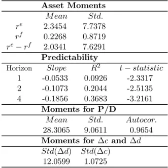
Table 1 presents the stylized asset pricing facts that we will use to compare the different models under rational expectations and adaptive learning. The data set is the one used in Campbell (2002).4 The quarterly stock market data set is obtained from the nominal CRSP NYSE/AMEX Value Weighted Indices. The aggregate dividend series is extracted from these indices to
con-2See Carceles-Poveda and Giannitsarou (2005). 3
Convergence to the rational expectations solution under RLS, for both models, is achieved under certain conditions, which we omit here since these are always satisfied for all reasonable parametrizations. Convergence under CG is achieved for small gains. The details for the derivations of these conditions can be found in Evans and Honkapohja (2001), as well as in Carceles-Poveda and Giannitsarou (2005).
struct the quarterly dividend and stock return series. Following Campbell (2002), the price dividend ratio is constructed as the stock price index associated with returns excluding divi-dends, divided by the total dividends paid during the last four quarters. The nominal risk-free rate is the three-month quarterly T-Bill rate. The nominal stock return is deflated using cur-rent inflation and the nominal risk-free rate is deflated using the inflation next period. The consumption series corresponds to real per capita consumption of non-durables and services.
<TABLE 1 HERE >
Thefirst part of table 1 reports our estimates for the quarterly mean and standard deviation of stock returns, the risk-free rate and the equity premium in percentage terms. The stock return has been around 2.3 % per quarter against a risk-free rate of 0.2 %, leading to a quarterly premium of around 2 % during the postwar period. We also see a much higher volatility for the equity return and equity premium of around 7.6 %, in contrast to the volatility of around 1 % for the risk-free rate. Replicating thefirst and second asset moments still represents a challenge for standard rational expectations models.
The second panel of table 1 reports results from regressions of the k = 1,2,4 year ahead equity premium on the current log price dividend ratio divided by its standard deviation. Thus, the slope coefficients reflect the effect of a one standard deviation change in the log price dividend ratio on the cumulative excess returns in natural units. The table reports the regression slopes, the adjusted R2 and the t-statistic, adjusted for heteroskedasticity and serial correlation with the Newey-West method.5 As reflected by the table, the predictive regressions exhibit the familiar pattern of an increasing R2 and coefficient slope for longer horizons. The fact that the log price dividend ratio predicts future excess returns was first documented by Fama and French (1988) and Campbell and Shiller (1988) and it still poses a puzzle for standard rational expectations models.
Finally, since the price dividend ratio is a crucial variable for addressing the predictability puzzle, the third panel of the table displays its mean, standard deviation and first order auto-correlation in levels. Furthermore, the last panel reports the standard deviation of consumption and dividend growth. It is important to note that these two variables are the same in the endowment economy, but they have a very different behavior in the data. Given this, we will only be able to match one of them with a single calibration.
5. Numerical Results
This section presents the numerical results for the two models under rational expectations and adaptive learning. For each of the two models, we calculate the same statistics as the ones
5For the truncation lag, we follow Campbell, Lo and MacKinlay (1997), who use q= 2 (k
−1). The results are very similar if we use q = k−1or the default value of q =f loor³4(T /100)2/9´ suggested to Eviews by
Newey and West. Similar qualitative results can be obtained by regressing thek-period ahead stock returns on the current log price dividend ratio.
reported in table 1. Additionally, we report the ratio of the standard deviation of the price under learning over the standard deviation under rational expectations, as a proxy for the stock price volatility generated by adaptive learning.
We begin by describing the computing specifications. To implement the simulations we have used the adaptive learning toolbox for Matlab that accompanies Carceles-Poveda and Giannitsarou (2005). For each model, we run experiments with a number of T = 211periods, corresponding to the number of quarters available from our data set. Furthermore, the statistics reported are the average statistics from replicating the experimentsN = 1000 times. To make all results comparable, shocks are generated from normal distributions with the same state value for theMatlab pseudorandom number generator, which was set to 98.
As shown in Carceles-Poveda and Giannitsarou (2005), the initialization of adaptive learning algorithms can have important effects on the model dynamics. We therefore use two different initializations. In the first, the initial elasticity φ0 is drawn from a distribution around the rational expectations equilibrium φ¯, with a variance which approximates the variance of an OLS estimator ofφbased on five observations. In the second,φ0 is set at a value that is below, above and exactly at the rational expectations value. These three values correspond to different initial priors of the households about the effects of the state variables on the current stock price. Finally, for each set of experiments, we simulate series under RLS learning and CG learning using gain coefficients of g = 0.02, g = 0.2 and g = 0.4. Our choice of these gain values is based on the interpretation of CG learning. As explained earlier, the CG algorithm assigns geometrically decreasing weights to observations across time, so that recent observations matter a lot for the current estimate, even in the limit. In this sense, we can interpret the constant gain algorithm as the tool of an econometrician that believes that recent observations are more relevant for forecasting than observations that date very far back. Specifically, an observation that datesiperiods back is assigned a weight equal to (1−g)i−1.
The size of the gain g corresponding to a weight of approximately zero for observations that date more than i years back is displayed in table 2.6 For example, if the econometrician
believes that only observations that date i= 15 years back are important for the forecast, the corresponding gain is g= 0.46, or ifi= 20years, theng = 0.37. Since professional forecasters typically use rather short and recent data series from the stock markets, we believe that a constant gain learning (with a relatively high gain coefficient) is a more appropriate modeling framework for asset pricing forecasting. Given this, we have calculated our results with gain values of 0.2 and 0.4, corresponding approximately to using data from the last 20 to 50 years. Furthermore, to get a sense of how our results depend on the size of the gain, we have also calculated the results with a gain ofg= 0.02, corresponding to approximately using data from the last 400 years to make the forecasts.
<TABLE 2 HERE >
6
Wefirst present the results for the endowment economy and then discuss the results for the production economy.
5.1. The Endowment Economy. In the endowment economy, the risk aversion value is set to γ = 1. Further, since use a quarterly time period, we setβ = 0.99. As for the dividend process, the benchmark calibration assumes thatρ= 0.95and σε = 0.06, corresponding to the
estimated slope coefficient and error standard deviation of regressing the log of the seasonally adjusted real dividend series in the data on its first lag. We also repeat the experiments with ρ = 0.95 and σε = 0.00712 in order to make the findings comparable to those from the
production economy. Moreover, this last calibration approximately replicates the behavior of logged consumption growth in the data.
Tables 3A-3C contain the results for the calibration with the lower variance, whereas tables 3D-3F report the same results for the higher shock variance. Tables 3A and 3D contain thefirst and second asset moments. Tables 3B and 3E contain (a) the standard deviation of the stock price under learning over the standard deviation of the stock price under rational expectations, (b) the average price dividend ratio, its standard deviation and itsfirst autocorrelation, (c) the standard deviation of consumption growth and (d) the standard deviation of dividend growth. Finally, tables 3C and 3F report the results for predictability. To obtain these, we run the same regressions as with the true data. The table reports the average estimated slope coefficients, the average adjusted R2 and the percentage of estimated coefficients that are negative and significant out of 1000replications of the experiment.
The first two rows of the tables display the numbers in the data and under rational ex-pectations (RE). Furthermore, the last six rows display the results under learning when the algorithms are initialized (a) from a distribution (DIS), (b) below the REE, with an elasticity set to 0.9×φ¯ (AH-B), or (c) above the REE, with an elasticity set to 1.035×φ¯ (AH-A).7 For each initialization, we report the results for the recursive least squares (RLS) and constant gain (CG) algorithms with gains of g = 0.2 and g = 0.4. The case with g = 0.02 is omitted, since the results are almost identical to the ones under RLS.
<TABLES 3A - 3F HERE>
Starting with the results under RE, we see that the model performs very poorly in all dimensions. With the lower shock variance, the premium is only around 0.002 percent, while it only increases to approximately 0.2 percent with the benchmark parameterization. Furthermore, whereas the standard deviation and the autocorrelation of the price dividend ratio are far from the data, this variable generates absolutely no predictability for the excess stock returns. This
7The percentage1.035above the REE has been chosen for both models, so that the stationarity condition
|φ0|<1is satisfied for the production economy. Although such a restriction is not necessary for the endowment economy, we use the same number to keep the results comparable. Furthermore, the case where the initial elasticity starts at the rational expectations valueφ has been omitted, since it generates the same results on average as when we initialize from a distribution.
is not surprising, since it is well documented in the literature that the Lucas tree model with a low risk aversion parameter value is unsuccessful in reproducing the asset pricing moments in the data.
Turning to the results under adaptive learning, the first important observation is that they are almost identical across the different initializations. In other words, different initial priors for the elasticity of the stock price with respect to the stochastic dividend process do not alter the results in the endowment economy. On the other hand, we do observe important differences across the different learning algorithms and parametrizations. We discuss the results with each algorithm in turn.
Starting with RLS learning, we see that the asset return moments are very close to those generated by rational expectations. In general, the reason why RLS cannot generate any sig-nificant improvements in the predictions of the model is that the algorithm converges relatively fast to the rational expectations equilibrium. Therefore, any differences between the dynamics under RLS and rational expectations disappear quickly. This is also reflected in tables 3B and 3E, illustrating that the standard deviation of the price under RLS learning over the one un-der rational expectations is approximately one with both parametrizations. Finally, Tables 3C and 3F illustrate that the model under RLS also performs very poorly regarding predictability. Whereas the coefficients have the right sign and are higher in absolute value than the ones under rational expectations, they are still far from the data under both calibrations. In addition, the percentage of significant simulations is relative small.
It should be pointed out that if we had also assumed that agents estimate the exogenous dividend process, some additional variation between RLS and rational expectations would be present. However, we have chosen not to allow learning on the exogenous dividend process for several reasons. First, since the dividend process is endogenous in the stochastic growth model, this would involve introducing some form of structural learning, while we want to focus on self-referential learning. Moreover, since the least squares estimates for the dividend process would be reached quite fast, we conjecture that this addition would not provide any significant variations, unless the assumed time horizon was very short.
With this discussion in mind, it should be clear that any improvements in the predictions of the model can only come from some type of learning algorithm that does not converge to the rational expectations equilibrium. Constant gain learning is such an algorithm, since its dynamicsfluctuate perpetually around the rational expectations equilibrium and the size of the fluctuations depends positively on the size of the gain function. Indeed, turning to the results generated by CG learning, the results appear to be quite different from those under RLS and rational expectations.
Whereas the improvements regarding the asset return moments are again relatively modest, we see a considerable improvement regarding the stock price volatility and predictability. Tables 3B and 3E reflect that the asset price under CG learning can be significantly more volatile than
under rational expectations. In addition, with the benchmark parameterization and the higher gain, the model matches the standard deviation of the logged dividend growth, whereas the standard deviation of the price-dividend ratio is just about half of the one observed in the data. Finally, tables 3C and 3F reflect that the model performs much better than under rational expectations regarding predictability. As we see, the average slope coefficients, the percentage of significant and negative estimates and the R2 display the increasing pattern with a longer horizon that we see in the data. Furthermore, the slope coefficients are surprisingly close to the ones in the data when the model is calibrated to dividend behavior (σ = 0.06) and the gain is equal to 0.4. In this case, the number of significant estimates in this case ranges from approximately 40% to 70%, a large improvement compared to the results under RLS and rational expectations.
These improvements are smaller when the model is calibrated to consumption behavior (σ = 0.00712). In this case, the model does not generate the right behavior for the dividend growth or the price dividend ratio. Further, although this calibration leads to a higher stock price volatility and generates a much higher predictability under learning than the rational expectations version, the slope coefficients with a gain of 0.4 do not provide a satisfactory match with the data.
Summarizing, RLS learning generates results that are very close to their rational expecta-tions counterpart. On the other hand, CG generates some improvements when the model is calibrated to dividend behavior, particularly with respect to the stock price volatility and the predictability of excess returns. In what follows, we provide some intuitive comments to help understand our findings.
Considerfirst the volatility of the stock price. It is easy to see that the variance of the price under rational expectations is only affected by the variance of the shock, since it is equal to
V ar(pret ) =V(φ)2V ar(zt) =V ar(zt). (31)
On the other hand, under adaptive learning, the behavior of the estimated coefficient φ also affects the price variance, which is given by
V ar(palt ) =a2V ar¡φt−1zt¢+b2V ar(zt) + 2ab Cov(φt−1zt). (32)
The variance in (32) will be higher than variance of the shock in (31) if V ar¡φt−1zt ¢
> V ar¡φzt
¢
, whereas the opposite will happen if V ar¡φt−1zt ¢
< V ar¡φzt ¢
. Our numerical results show that V ar¡φt−1zt¢ is on average very similar to V ar¡φzt¢ under RLS, explaining
why the two prices have almost the same variability. For the case of CG learning, however, the coefficients deviate more from the REE solution, and V ar¡φt−1zt
¢
is on average higher than V ar¡φzt
¢
, explaining the higher price variability. Finally, sinceV ar¡φt−1zt ¢
is increasing with the variability of φt−1, which increases with a higher gain, this would also explain the higher
variance of the price with higher gain coefficients.
While learning may generate some extra volatility with a high gain, note that the mean equity premium is very close to its value under rational expectations. To see why this is the case, note that the expected equity premium under rational expectations is given by8
rrpt+1 =γηczηre
z V ar(zt), (33)
where ηcz and ηre
z represent the elasticities of the unexpected consumption growth and the
unexpected equity return with respect to the shock. Moreover, these elasticities depend on the deep parameters of the model and on the underlying elasticity φ¯. First, similar arguments to the ones for volatility can be used to explain why more volatile estimated coefficients can generate some extra excess return volatility through their effects on the two elasticitiesηcz and ηre
z. However, since the estimated coefficients are on average close to their REE values, the
consumption and equity return elasticities will not be very far from the REE solution. We therefore conclude that, unless some form of misspecification is introduced, standard adaptive learning does not have a lot of potential for explaining mean returns in the present model.
Finally, to explain why self-referential learning can generate excess return predictability, note that the actual law of motion for the price under learning is given by
pt=T ¡ φt−1¢zt−1+V ¡ φt−1¢εt=V ¡ φt−1¢zt, (34) where T¡φt−1¢ = ¡aφt−1+b¢ρ, (35) V ¡φt−1¢ = ¡aφt−1+b¢.
Consider an estimate ofφthat is below the "true" or rational expectations value. SinceV ¡φt−1¢ is increasing in φt−1, the stock price will be low and this will generate a low price to dividend ratio (or a high dividend to price ratio) which, in turn, will generate higher future returns. This is because, first, a higher dividend to price ratio implies higher payoffs and, second, because when the price re-adjusts upwards, it will lead to higher capital gains. A similar argument would indicate that an estimate of φ that is above the true value will lead to a higher than average price to dividend ratio and to lower future returns. This indicates that learning has the potential of generating a negative correlation between the current price to dividend ratio and the future excess returns. Finally, it is worth noting that φ and V (φ) are constant under rational expectations. This implies that the effects we have just described are not present in the fully rational setting, providing a possible explanation for its poor performance concerning predictability.
5.2. The Production Economy. For the production economy, we have used the standard parametrization for US quarterly data. The risk aversion coefficient is again set to γ = 1. Furthermore, the capital depreciation, the discount factor and the capital share are set to δ = 0.025, β = 0.99 and α= 0.36 respectively. Finally, regarding the productivity shock, our baseline parametrization is σε = 0.00712 and ρ = 0.95, as is usual in the real business cycle
literature.
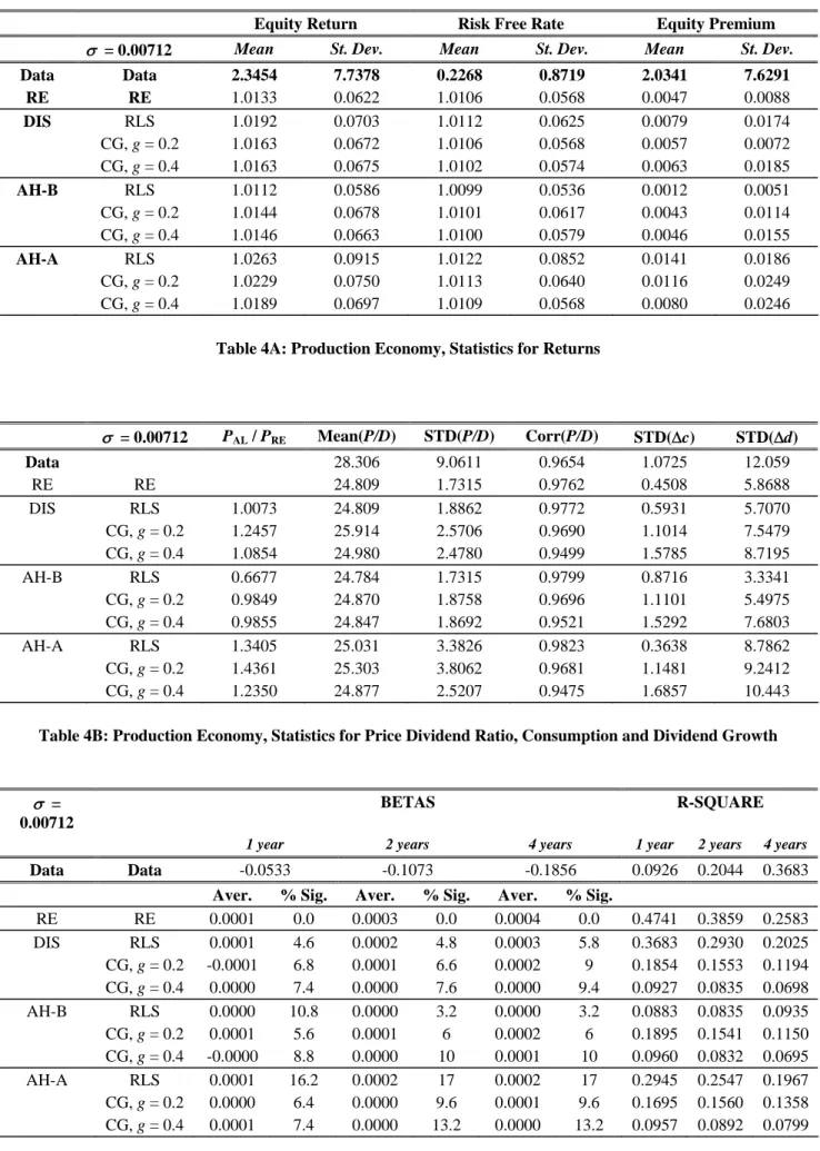
Tables 4A-4C report the results for the production economy, organized in the same way as the results for the endowment economy. In particular, table 4A contains asset moments, table 4B contains various statistics and table 4C reports the results for predictability.
< TABLES 4A - 3C HERE>
As with the endowment economy, the tables indicate that the rational production economy performs very poorly in explaining the first and second asset moments.9 The implied equity premium is approximately 0.005 percent, whereas the asset variabilities are very similar across the two assets and very far from their counterparts in the data. Furthermore, the standard deviation of the price dividend ratio is much lower than the one in the data, and it does not have any predictive power for the excess stock returns.
Turning to the results under learning, we see that it has a very small effect on the different asset moments. In particular, the equity premium only increases from 0.005 to 0.01 percent and its variability only increases from 0.01 to 0.025 percent. In addition, constant gain learning does induce stock price volatility, but this seems to be non-monotonic with respect to the gain coefficient. Finally, although learning improves the behavior of the price dividend ratio, the average regression coefficients are practically zero and rarely significant for all the horizons con-sidered, as can be seen from table 4C. Thesefindings suggest that, with a standard calibration, adaptive learning does not seem to provide an explanation for the behavior of asset returns in the production economy.
An interesting observation is that the results depend on the different initializations of the learning algorithms, unlike in the endowment economy. In particular, starting above the rational expectations value generates a premium that is ten times higher than the premium if we start below rational expectations. This is also reflected in the relative variability of the stock price. As can be seen in Table 4B, the variability of the stock price can be considerably lower than under rational expectations if the initial coefficient is set below its rational expectations value, while it is always higher if we start above. Thus, contrary to the common view that learning can only generate higher volatility, we find that the size of the volatility actually depends on the initialization of the algorithm in the stochastic growth model and may very well be below the one generated by rational expectations.10
9
See for example Rouwenhorst (1995), or Lettau (2003).
1 0An extensive discussion of the effects of different initializations of learning can be found in Carceles-Poveda
In what follows, we discuss intuitively why adaptive learnings fails to improve the predictions of the model in the production economy. First, regarding the volatility of asset prices, it can be shown that it is equal to the following expression under rational expectations:11
V ar(preet ) = γ 2(1 +ρφ¯ p) (1−a1ρ−a1φ¯p)2(1−ρφ¯p)(1−φ¯ 2 p) (36)
Moreover, for our calibration, it is possible to show that the previous expression is increasing in φ¯p. Using this result, we can then heuristically argue that the variance of the endogenous state under learning will be lower than the variance under rational expectations if the estimated coefficientsφp remain well belowφ¯p for a large number of periods.
If we initialize the algorithm using a distribution, RLS implies that these coefficients will be relatively close to the REE, leading to a very similar variance between the two cases. On the other hand, a gain of 0.2 makes them more volatile, so that they are more often above the REE. Finally, increasing the gain coefficient above 0.2 also implies that the coefficients violate the stationarity condition requiring that ¯¯φp,t−1¯¯ < 1, since the REE value φ¯p is very close to one. Since it would not be sensible to allow the elasticity to be larger than one, the learning algorithm is augmented with a projection facility, which simply resets φ to its last value when this condition is violated. In this case, the projection facility generates a downward bias that reduces the price volatility when increasing the gain from 0.2 to 0.4, explaining the non-monotonicity in the results that is seen in the tables.12
On the other hand, if we initialize the algorithm above or below the REE, the estimated coefficients will remain on average above or below the REE respectively. This happens because of persistence, which due to the presence of a lag in the law of motion of the stock price. This explains why the different initializations generate different results in the production economy, while they do not matter in the endowment economy.
Finally, turning to the predictability results, note that the actual law of motion for the price in the production economy is given by
pt=T(φt−1)pt−1+V(φt−1)zt, (37) where T(φ) = a2 1−a1φp , (38) V(φ) = a1φz+b 1−a1φp .
1 1See Giannitsarou (2005) for a derivation. 1 2
For details on the projection facility and how it affects the behavior of the estimates see Carceles-Poveda and Giannitsarou (2005). Note that we do not need to impose it in the endowment economy, where the equilibrium is globally stable.
Comparing to the case of the endowment economy, a lower estimate of φz,t−1 does not directly translate into a lower than average price level anymore, since the T and V maps are also affected by φp,t−1. In particular, our numerical results suggest that these two coefficients move on average in opposite directions, whereas their variances are similar. Thus, while a lower estimate of φz leads to a lowerV(φt−1) and therefore to a lower price, a higher estimate of φp has the opposite effect, since it increases V(φt−1) and T(φt−1). Moreover, as noted earlier, the elasticity of the price with respect to the shock is much smaller than that in the endowment economy. Based on these arguments, these findings suggest that any effects learning might induce may cancel out for all algorithms when the variance of the shock is relatively small.
Yet, a higher shock variance could generate some better results in this respect, since it will lead to a higher feedback of the estimate of φz,t−1 on the price through a higher second term V(φt−1)zt. To get a sense of how big such an effect would be, we have also simulated
the production economy with a higher shock variance.13 In this case, we find that a higher
shock variance generates some predictability, especially with the initialization above the REE. In particular, the estimated slope coefficients in this case can be around one half of their value in the data. The number of significant simulations, however, is still considerably smaller than in the endowment economy. In addition, wefind that the model can generate a higher premium and return volatility than under rational expectations, specially with the initialization above the rational expectations equilibrium. As before, this can be explained by the persistence induced by the lag in the law of motion of the price, which implies that the elasticities that affect the equity premium are further away from their rational expectations value than in the endowment economy. Of course, such improvements come at the expense of unrealistically high values for the moments of the price dividend ratio and of the real macroeconomic variables. Given this, we conclude that learning does not provide a satisfactory explanation for the asset pricing puzzles in the presence of capital accumulation.
6. Conclusion
We studied the effects of self-referential adaptive learning on asset returns in the framework of standard general equilibrium asset pricing models. In particular, we have considered recursive least squares and constant gain learning, with a variety of specifications, in a production econ-omy and a Lucas type exchange econecon-omy. Both models were evaluated with respect to thefirst and second equity premium moments, the predictability of excess returns and the volatility of stock prices. The main conclusions from our results are that (a) constant gain adaptive learning has a chance of generating stock price volatility and predictability in the endowment economy, when the gain coefficient is relatively high, (b) constant gain learning does not generate any interesting improvements in the production economy framework and (c) recursive least squares learning does not generate any improvements for any of the two models.
1 3To avoid the proliferation of tables, we do not report the results of these simulations but they can be provided
In general, standard adaptive learning has little potential of explaining the mean excess returns in the data, since the average estimated coefficients from the law of motion of the stock price fluctuate around the rational expectations equilibrium, which is known to fail in generating a sizeable premium for reasonable parametrizations. As to the stock price volatility and predictability of excess returns, we find important differences across models and across learning algorithms. In particular, recursive least squares learning has relatively small effect on the stock price volatility and it generates no predictability in the production economy and almost no predictability in the endowment economy. The effects of constant gain learning with a relatively small gain are very similar. Nevertheless, a higher gain coefficient, reflecting the fact that forecasters give more importance to recent observations, generates considerably more volatility and predictability in the endowment economy, especially when it is calibrated to match the dividend behavior in the data.
In general, our findings suggest that tracking algorithms such as CG have more potential than RLS to explain asset pricing facts in models where there is no inherent persistence in the stock price, such as the Lucas Tree endowment economy. On the other hand, in the presence of capital accumulation, where the endogenous variables exhibit more persistence and where consumption smoothing plays an important role, adaptive learning is not sufficient to generate any of the stylized facts in the data.
A. Reduced Form Coefficients The coefficients of the reduced form for the production economy are
a1 = − γ γ(−2 +δ−αψ) + (δ−ψ) (1 +β(δ−1−α2ψ)), (39a) a2 = γ(δ−1−αψ) γ(−2 +δ−αψ) + (δ−ψ) (1 +β(δ−1−α2ψ)), (39b) b = ψ(γ(ρ−1) +αβ(δ−ψ)ρ) γ(−2 +δ−αψ) + (δ−ψ) (1 +β(δ−1−α2ψ)), (39c) whereψ= (1−β+δβ)/(αβ). References
[1] Brennan, M. J. and Y. Xia, 2001. Stock Price Volatility and Equity Premium. Journal of Monetary Economics, 47, 249-283.
[2] Brock, W. A. and C. H. Hommes, 1998. Heterogeneous Beliefs and Routes to Chaos in a Simple Asset Pricing Model.Journal of Economic Dynamics and Control, 22, 1235-1274. [3] Bullard, J. and J. Duffy, 2001. Learning and Excess Volatility.Macroeconomic Dynamics,
[4] Campbell, J. Y., 2003. Consumption-Based Asset Pricing. In the Handbook of the Eco-nomics of Finance,Elsevier North-Holland.
[5] Campbell, J. Y., A. W. Lo and A. G. MacKinlay, 1997. The Econometrics of Financial Markets. Princeton University Press.
[6] Campbell, J. and R. Shiller, 1988, Stock Prices, Earnings and Expected Dividends,Journal of Finance 43(3), 661-676.
[7] Carceles-Poveda, E., 2005, Idiosyncratic Shocks and Asset Returns in the RBC Model, an Approximate Analytical Approach, Macroeconomic Dynamics, forthcoming.
[8] Carceles-Poveda, E. and C. Giannitsarou, 2005. Adaptive Learning in Practice. Mimeo-graph.
[9] Cecchetti, S., P. S. Lam and N. C. Mark, 2000. Asset Pricing with Distorted Beliefs: Are Equity Returns Too Good to be True?.American Economic Review, 90, 787-805.
[10] Evans, G. and S. Honkapohja, 2001. Learning and Expectations in Macroeconomics. Prince-ton University Press.
[11] Fama E. and K. French, 1988, Dividend Yields and Expected Stock Returns, Journal of Financial Economics 22(1), 3-27.
[12] Giannitsarou, C., 2005, E-stability Does Not Imply Learnability,Macroeconomic Dynamics 9, 276-287.
[13] Honkapohja, S. and K. Mitra, 2003. Learning with Bounded Memory in Stochastic Models. Journal of Economic Dynamics and Control, 27, 1437-1457.
[14] Kocherlakota N., 1996, The Equity Premium: It’s still a Puzzle, Journal of Economic Literature, Vol. 34, No. 1, pp. 42-71.
[15] Lettau M., 2003, Inspecting the Mechanism: The Determination of Asset Prices in the Real Business Cycle Model,The Economic Journal, 113, 550—575.
[16] Rouwenhorst K. G., 1995, Asset Prices Implications of Equilibrium Business Cycle Mod-els. In New Frontiers of Modern Business Cycle Research, ed. by T. Cooley, Princeton University Press.
[17] Shiller, R. J., 1989. Market Volatility. MIT Press.
[18] Timmermann, A., 1994. How Learning in Financial Markets Generates Excess Volatility and Predictability in Stock Prices.Quarterly Journal of Economics, 108, 1135-1145.
[19] Timmermann, A., 1996. Excess Volatility and Predictability of Stock Prices in Autoregres-sive Dividend Models with Learning.Review of Economic Studies, 63, 523-557.
Asset Moments M ean Std. re 2.3454 7.7378 rf 0.2268 0.8719 re−rf 2.0341 7.6291 Predictability
Horizon Slope R2 t−statistic
1 -0.0533 0.0926 -2.3317 2 -0.1073 0.2044 -2.5135 4 -0.1856 0.3683 -3.2161 Moments for P/D M ean Std. Autocor. 28.3065 9.0611 0.9654 Moments for ∆c and ∆d Std(∆d) Std(∆c)
12.0599 1.0725
Table 1: Asset pricing facts 1947.2-1998.4
Y ears 400 200 100 50 25 20 15 10 5 Gain 0.02 0.04 0.09 0.17 0.31 0.37 0.46 0.60 0.85
σ = 0.00712 Mean St. Dev. Mean St. Dev. Mean St. Dev. Data 2.3454 7.7378 0.2268 0.8719 2.0341 7.6291 RE 1.0123 0.7303 1.0106 0.1020 0.0017 0.7562 DIS RLS 1.0122 0.7156 1.0106 0.1020 0.0017 0.7424 CG, g = 0.2 1.0128 0.7629 1.0106 0.1020 0.0024 0.7911 CG, g = 0.4 1.0146 0.8788 1.0106 0.1020 0.0043 0.9067 AH-B RLS 1.0122 0.7143 1.0106 0.1020 0.0017 0.7459 CG, g = 0.2 1.0128 0.7646 1.0106 0.1020 0.0024 0.7928 CG, g = 0.4 1.0146 0.8810 1.0106 0.1020 0.0043 0.9089 AH-A RLS 1.0122 0.7143 1.0106 0.1020 0.0017 0.7459 CG, g = 0.2 1.0128 0.7646 1.0106 0.1020 0.0024 0.7928 CG, g = 0.4 1.0146 0.8810 1.0106 0.1020 0.0043 0.9089
Table 3A: Endowment Economy, Statistics for Returns
σ = 0.00712 PAL / PRE Mean(P/D) STD(P/D) Corr(P/D) STD(Δc) STD(Δd) Data 28.3065 9.0611 0.9654 1.0725 12.0599 RE 24.7521 0.1639 0.5395 1.4432 1.4432 DIS RLS 0.9895 24.7531 0.1944 0.6554 1.4432 1.4432 CG, g = 0.2 1.1516 24.7542 0.2806 0.7909 1.4432 1.4432 CG, g = 0.4 1.4138 24.7631 0.4398 0.8642 1.4432 1.4432 AH-B RLS 0.9949 24.7542 0.1903 0.6437 1.4432 1.4432 CG, g = 0.2 1.1544 24.7548 0.2805 0.7899 1.4432 1.4432 CG, g = 0.4 1.4180 24.7633 0.4415 0.8642 1.4432 1.4432 AH-A RLS 0.9949 24.7542 0.1903 0.6437 1.4432 1.4432 CG, g = 0.2 1.1544 24.7548 0.2805 0.7899 1.4432 1.4432 CG, g = 0.4 1.4180 24.7633 0.4415 0.8642 1.4432 1.4432
Table 3B: Endowment Economy, Statistics for Price Dividend Ratio, Consumption and Dividend Growth
BETAS R-SQUARE
σ = 0.00712 1 year 2 years 4 years 1 year 2 years 4 years
Data -0.0533 -0.1073 -0.1856 0.0926 0.2044 0.3683
Aver. % Sig. Aver. % Sig. Aver. % Sig.
RE -0.0000 7.6 -0.0001 10 -0.0002 14.4 0.0046 0.0056 0.0057 DIS RLS -0.0005 7 -0.0009 11.6 -0.0017 17.8 0.0066 0.0119 0.0205 CG, g = 0.2 -0.0234 16.4 -0.0477 31.8 -0.0083 45.2 0.0207 0.0432 0.0722 CG, g = 0.4 -0.0049 44.4 -0.0093 59.2 -0.0152 67.8 0.0561 0.0983 0.1424 AH-B RLS -0.0004 6.8 -0.0008 12 -0.0015 16.4 0.0064 0.0106 0.0179 CG, g = 0.2 -0.0233 17.8 -0.0475 31.8 -0.0082 44.8 0.0205 0.0424 0.0713 CG, g = 0.4 -0.0049 43.8 -0.0093 60 -0.0153 68 0.0561 0.0982 0.1424 AH-A RLS -0.0004 6.8 -0.0008 12 -0.0015 16.4 0.0064 0.0106 0.0179 CG, g = 0.2 -0.0233 17.8 -0.0475 31.8 -0.0082 44.8 0.0205 0.0424 0.0713 CG, g = 0.4 -0.0049 43.8 -0.0093 60 -0.0153 68 0.0561 0.0982 0.1424
Equity Return Risk Free Rate Equity Premium σ = 0.06 Mean St. Dev. Mean St. Dev. Mean St. Dev.
Data 2.3454 7.7378 0.2268 0.8719 2.0341 7.6291 RE 1.1940 6.1721 1.0185 0.8600 0.1769 6.3894 DIS RLS 1.1984 6.0497 1.0185 0.8600 0.1813 6.2752 CG, g = 0.2 1.2389 6.4672 1.0185 0.8600 0.2226 6.7052 CG, g = 0.4 1.4244 7.7093 1.0185 0.8600 0.4088 7.8943 AH-B RLS 1.1974 6.0808 1.0185 0.8600 0.1805 6.3049 CG, g = 0.2 1.2386 6.4812 1.0185 0.8600 0.2224 6.7188 CG, g = 0.4 1.4115 7.6763 1.0185 0.8600 0.3959 7.9095 AH-A RLS 1.1974 6.0808 1.0185 0.8600 0.1805 6.3049 CG, g = 0.2 1.2386 6.4812 1.0185 0.8600 0.2224 6.7188 CG, g = 0.4 1.4115 7.6763 1.0185 0.8600 0.3959 7.9095
Table 3D: Endowment Economy, Statistics for Returns
σ = 0.06 PAL / PRE Mean(P/D) STD(P/D) Corr(P/D) STD(Δc) STD(Δd) Data 28.3065 9.0611 0.9654 1.0725 12.0599 RE 24.7621 1.3805 0.5390 12.187 12.187 DIS RLS 0.9895 24.7941 1.6589 0.6566 12.187 12.187 CG, g = 0.2 1.1516 24.8985 2.4223 0.7898 12.187 12.187 CG, g = 0.4 1.4138 24.4047 4.6046 0.8599 12.187 12.187 AH-B RLS 0.9949 24.7995 1.6084 0.6432 12.187 12.187 CG, g = 0.2 1.1544 24.9028 2.4219 0.7887 12.187 12.187 CG, g = 0.4 1.4180 24.4083 4.6187 0.8528 12.187 12.187 AH-A RLS 0.9949 24.7995 1.6084 0.6432 12.187 12.187 CG, g = 0.2 1.1544 24.9028 2.4219 0.7887 12.187 12.187 CG, g = 0.4 1.4180 24.4083 4.6187 0.8528 12.187 12.187
Table 3E: Endowment Economy, Statistics for Price Dividend Ratio, Consumption and Dividend Growth
BETAS R-SQUARE
σ = 0.06 1 year 2 years 4 years 1 year 2 years 4 years
Data -0.0533 -0.1073 -0.1856 0.0926 0.2044 0.3683
Average % Sig. Average % Sig. Average % Sig. RE -0.0001 7.8 -0.0008 10.2 -0.0017 14 0.0045 0.0056 0.0057 DIS RLS -0.0041 7.2 -0.0083 11.8 -0.0144 18 0.0066 0.0119 0.0205 CG, g = 0.2 -0.0198 16.6 -0.0403 32.4 -0.0701 45.9 0.0217 0.0430 0.0725 CG, g = 0.4 -0.0443 43.6 -0.0834 60.4 -0.1362 68.2 0.0578 0.1016 0.1449 AH-B RLS -0.0035 7 -0.0071 12 -0.0127 17 0.0064 0.0106 0.0179 CG, g = 0.2 -0.0197 18.2 -0.0401 32.4 -0.0700 54.8 0.0215 0.0426 0.0716 CG, g = 0.4 -0.0442 43.4 -0.0831 64.2 -0.1357 68.6 0.0579 0.1006 0.1457 AH-A RLS -0.0035 7 -0.0071 12 -0.0127 17 0.0064 0.0106 0.0179 CG, g = 0.2 -0.0197 18.2 -0.0401 32.4 -0.0700 54.8 0.0215 0.0426 0.0716 CG, g = 0.4 -0.0442 43.4 -0.0831 64.2 -0.1357 68.6 0.0579 0.1006 0.1457
Equity Return Risk Free Rate Equity Premium
σ = 0.00712 Mean St. Dev. Mean St. Dev. Mean St. Dev. Data Data 2.3454 7.7378 0.2268 0.8719 2.0341 7.6291 RE RE 1.0133 0.0622 1.0106 0.0568 0.0047 0.0088 DIS RLS 1.0192 0.0703 1.0112 0.0625 0.0079 0.0174 CG, g = 0.2 1.0163 0.0672 1.0106 0.0568 0.0057 0.0072 CG, g= 0.4 1.0163 0.0675 1.0102 0.0574 0.0063 0.0185 AH-B RLS 1.0112 0.0586 1.0099 0.0536 0.0012 0.0051 CG, g = 0.2 1.0144 0.0678 1.0101 0.0617 0.0043 0.0114 CG, g = 0.4 1.0146 0.0663 1.0100 0.0579 0.0046 0.0155 AH-A RLS 1.0263 0.0915 1.0122 0.0852 0.0141 0.0186 CG, g = 0.2 1.0229 0.0750 1.0113 0.0640 0.0116 0.0249 CG, g = 0.4 1.0189 0.0697 1.0109 0.0568 0.0080 0.0246
Table 4A: Production Economy, Statistics for Returns
σ = 0.00712 PAL / PRE Mean(P/D) STD(P/D) Corr(P/D) STD(Δc) STD(Δd) Data 28.306 9.0611 0.9654 1.0725 12.059 RE RE 24.809 1.7315 0.9762 0.4508 5.8688 DIS RLS 1.0073 24.809 1.8862 0.9772 0.5931 5.7070 CG, g = 0.2 1.2457 25.914 2.5706 0.9690 1.1014 7.5479 CG, g= 0.4 1.0854 24.980 2.4780 0.9499 1.5785 8.7195 AH-B RLS 0.6677 24.784 1.7315 0.9799 0.8716 3.3341 CG, g = 0.2 0.9849 24.870 1.8758 0.9696 1.1101 5.4975 CG, g = 0.4 0.9855 24.847 1.8692 0.9521 1.5292 7.6803 AH-A RLS 1.3405 25.031 3.3826 0.9823 0.3638 8.7862 CG, g = 0.2 1.4361 25.303 3.8062 0.9681 1.1481 9.2412 CG, g = 0.4 1.2350 24.877 2.5207 0.9475 1.6857 10.443
Table 4B: Production Economy, Statistics for Price Dividend Ratio, Consumption and Dividend Growth
σ = 0.00712
BETAS R-SQUARE
1 year 2 years 4 years 1 year 2 years 4 years
Data Data -0.0533 -0.1073 -0.1856 0.0926 0.2044 0.3683
Aver. % Sig. Aver. % Sig. Aver. % Sig.
RE RE 0.0001 0.0 0.0003 0.0 0.0004 0.0 0.4741 0.3859 0.2583 DIS RLS 0.0001 4.6 0.0002 4.8 0.0003 5.8 0.3683 0.2930 0.2025 CG, g = 0.2 -0.0001 6.8 0.0001 6.6 0.0002 9 0.1854 0.1553 0.1194 CG, g = 0.4 0.0000 7.4 0.0000 7.6 0.0000 9.4 0.0927 0.0835 0.0698 AH-B RLS 0.0000 10.8 0.0000 3.2 0.0000 3.2 0.0883 0.0835 0.0935 CG, g = 0.2 0.0001 5.6 0.0001 6 0.0002 6 0.1895 0.1541 0.1150 CG, g = 0.4 -0.0000 8.8 0.0000 10 0.0001 10 0.0960 0.0832 0.0695 AH-A RLS 0.0001 16.2 0.0002 17 0.0002 17 0.2945 0.2547 0.1967 CG, g = 0.2 0.0000 6.4 0.0000 9.6 0.0001 9.6 0.1695 0.1560 0.1358 CG, g = 0.4 0.0001 7.4 0.0000 13.2 0.0000 13.2 0.0957 0.0892 0.0799