A Latent Class Model for Discrete Choice Analysis: Contrasts with Mixed Logit

WORKING PAPER

ITS-WP-02-08

A Latent Class Model for

Discrete Choice Analysis:

Contrasts with Mixed Logit

By

William H Greene and David A Hensher

September, 2002

ISSN 1440-3501

INSTITUTE OF

TRANSPORT STUDIES

The Australian Key Centre in Transport Management The University of Sydney and Monash University

NUMBER:

Working Paper ITS-WP-02-08

TITLE:

A Latent Class Model for Discrete Choice Analysis:

Contrasts with Mixed Logit

ABSTRACT:

The multinomial logit model (MNL) has for many years

provided the fundamental platform for the analysis of discrete choice. The basic model’s several shortcomings, most notably its inherent assumption of independence from irrelevant alternatives (IIA) have motivated researchers to develop a variety of alternative formulations. The mixed logit model stands as one of the most significant of these extensions. This paper proposes a semi-parametric extension of the MNL, based on the latent class formulation, which resembles the mixed logit model but which relaxes its requirement that the analyst makes specific assumptions about the distributions of parameters across individuals. An application of the model to the choice of long distance travel by three road types (2-lane, 4-lane without a median and 4-lane with a median) by car in New Zealand is used to compare the MNL latent class model with mixed logit.

KEY WORDS: Choice models, mixed logit, latent class, stated choice. AUTHORS: William H Greene and David A Hensher

CONTACT: Institute of Transport Studies (Sydney & Monash) The Australian Key Centre in Transport Management, C37

The University of Sydney NSW 2006, Australia Telephone: +61 9351 0071

Facsimile: +61 9351 0088

Email: itsinfo@its.usyd.edu.au

Internet: http://www.its.usyd.edu.au

1. Introduction

The multinomial logit model (MNL) has for many years provided the fundamental platform for the analysis of discrete choice. The basic model’s several shortcomings, most notably its inherent assumption of independence from irrelevant alternatives (IIA) have motivated researchers to develop a variety of alternative formulations. The mixed logit model (McFadden and Train 2001) stands as one of the most significant of these extensions. This paper proposes a semi-parametric extension of the MNL, based on the latent class formulation, which resembles the mixed logit model but which relaxes its requirement that the analyst makes specific assumptions about the distributions of parameters across individuals. An application of the model to the choice of long distance travel by three road types (2-lane, 4-lane without a median and 4-lane with a median) by car in New Zealand is used to compare the MNL latent class model with mixed logit.

2. The Latent Class Model

The latent class model (LCM) for the analysis of individual heterogeneity has a history in several literatures. (See Heckman and Singer (1984) for theoretical discussion.) However, a review of the literature suggests that the vast majority of the received applications have been in the area of models for counts using the Poisson or negative binomial models. See Nagin and Land (1991) for an application and Greene (2001) for a survey of the literature. The model has had limited application to the analysis of discrete choice among multiple alternatives. The exception is Swait (1994).

The underlying theory of the latent class model posits that individual behavior depends on observable attributes and on latent heterogeneity that varies with factors that are unobserved by the analyst. We propose to analyze this heterogeneity through a model of discrete parameter variation. Thus, it is assumed that individuals are implicitly sorted into a set of Q classes, but which class contains any particular individual, whether known or not to that individual, is unknown to the analyst. The central behavioral model is a logit model for discrete choice among Ji alternatives, by individual i

observed in Tichoice situations,

,

, 1

exp(

)

Prob[choice by individual in choice situation | class ] =

exp(

)

i it j q J it j q j

j

i

t

q

=

′

′

∑

x

x

β

β

= F(i,t,j | q). (1) The number of observations and the size of the choice set may vary by individual. In principle, the choice set could vary by choice situation as well. The probability for the specific choice made by an individual can be formulated in several ways; for convenience, we allow yit to denote the specific choice made, so that the model provides

Pit | q(j) = Prob(yit = j | class = q). (2)

For convenience, we simplify this further to Pit | q. We have used a generic notation for

the density of the random variable of interest to suggest that this formulation will provide a means of extending the latent class model to other frameworks, though we

restrict our attention herein to the discrete choice model. Note that this is a ‘panel data’ sort of application in that we assume that the same individual is observed in several choice situations.

We assume that given the class assignment, the Ti events are independent. (This is a

possibly strong assumption, especially given the nature of the sampling design used in our application - a stated choice experiment in which the individual answers a sequence of survey questions. In fact, there might well be correlation in the unobserved parts of the random utilities. The latent class does not readily extend to autocorrelation, so we have left this aspect for further research.) Thus, for the given class assignment, the contribution of individual i to the likelihood would be the joint probability of the sequence yi = [yi1,yi2,...yiT]. This is | ₁ | i T i q _t it q P =

∏

₌ P (3)

The class assignment is unknown. Let Hiq denote the prior probability for class q for

individual i (we consider posterior probabilities below). Various formulations have been used this (see Greene 2001). For this application, a particularly convenient form is the multinomial logit:

( )

( )

1 exp , exp i q iq Q i q q H = ′ = ′

∑

z z θ θ q = 1,...,Q, θQ = 0, (4)

where zi denotes a set of observable characteristics which enter the model for class

membership. Roeder, Lynch and Nagin (1999), using this same formulation, denote zi

the ‘risk factors.’ The Qth parameter vector is normalized to zero to secure identification of the model (Greene 2003, Chapter 21). There may be no such covariates, in which case, the only element in zi would be the constant term, ‘1,’ and the

latent class probabilities would be simple constants which, by construction, sum to one. The likelihood for individual i is the expectation (over classes) of the class specific contributions: | 1 . Q i _q iq i q P =

∑

₌ H P (5)

The log likelihood for the sample is

ln L = N₁ln N₁ln Q₁

(

Ti_{1 |}

)

.

i iq it q

i= P = i=  q= H t= P 

∑

∑

∑

∏

(6)

Maximization of the log likelihood with respect to the Q structural parameter vectors, βq

and the Q-1 latent class parameter vectors, θq is a conventional problem in maximum

likelihood estimation. Greene (2001) discusses the mechanics and various aspects of estimation. In comparison to more familiar maximum likelihood problems, this is a relatively difficult optimization problem, though not excessively so. For a given choice of Q, the choice of good starting values seems to be crucial. The asymptotic covariance

matrix for the full set of parameter estimators is obtained by inverting the analytic second derivatives matrix of the log likelihood function.

An issue to be confronted is the choice of Q, the number of classes. This is not a parameter in the interior of a convex parameter space, so, for example, ‘testing down’ to the appropriate Q by comparing the log likelihoods of sequentially smaller models is not an appropriate approach. Nor is simply zeroing the coefficients of the Qth class, since setting the parameters to zero does not reduce the number of classes. Roeder et al. (1999) suggest using the Bayesian Information Criterion

BIC(model) = ln L + (model size) lnN

N (7)

With the parameter estimates of θq in hand, the prior estimates of the class probabilities

are ˆH_iq. Using Bayes theorem, we can obtain a posterior estimate of the latent class probabilities using | | | 1 ˆ ˆ ˆ ˆ ˆ i q iq q i Q i q iq q P H H P H = =

∑

(8)

A strictly empirical estimator of the latent class within which the individual resides would be that associated with the maximum value of Hˆ_{q i|} . We may also use these results to obtain posterior estimates of the individual specific parameter vector

| 1

ˆ Q ˆ ˆ

i=

∑

_q= Hq i q

β β . (9)

The same result can be used to estimate marginal effects in the logit model;

, | , | , ln ( , , | ) _{[1( ) ( , , | )]} km itj q it km m q it km F i t j q _{x j k F i t k q} x σ =∂ = = − β ∂ (10)

for the effect on individual i’s choice probability j in choice situation t of attribute m in choice probability k. The posterior estimator of this elasticity is

, | 1 ˆ | , |

ˆ_{km tj i} Q_q H_{q i}ˆ_{km ji q}

σ =

∑

₌ σ . (11)

An estimator of the average of this quantity over data configurations and individuals would be , _{1 1} , | 1 1 ˆ N Ti _{ˆ .} km j _{i t} km tj i i N T σ =

∑

₌

∑

₌σ (12)

3. The Mixed Logit Model

The mixed logit model (MLM) is similar to the LCM, but embodies several important differences as well. The central equation for the choice probability is

, , 1

exp( )

Prob[choice by individual in choice situation ] =

exp( ) i it j i J it j i j j i t = ′ ′

∑

x x β β = Pit|vi. (13) The K model parameters are continuously distributed across individuals with

βi = β + ∆zi + Γvi (14)

where

E[vi] = 0, Var[vi] = Σ = diag[σ1,…,σK] (15)

and where σk is a known constant. The variances and covariances of the joint

distribution of βi are parameterized in the unknown lower triangular matrix Γ which is

to be estimated. Since Γ is unknown, the assumption that σk is known is of no

consequence. Where parameters are marginally normally distributed, for example, σk =

1 while if they have a logistic distribution, σk = π2/3. The variance of the distribution of

the parameters is

Ω = ΓΣΓ′ (16) As before, Ti observations are made on each individual. The conditional contribution to

the likelihood is Pi|vi.= T_ti_{1 it} | i P =

∏

v (17)

In order to form the unconditional likelihood, it is necessary to integrate vi out of the

joint probability. Thus, | ( )

i

i i i i i

P =

_∫

P h d

v v v v (18)

where h(vi) is the density of the standardized random vector vi. This integral will

generally be intractable, even if vi is not a mixture of distributions, which it may be.

Recent applications have surmounted this difficulty be maximizing the simulated log likelihood function 1 1 1 lnLs _iN ln _rR ln |Pi ir R = =   = _{ }  

∑

∑

v (19)

where vir is a simulated random draw from the assumed distribution. (See Greene 2001,

Gourieroux et al., 1995 and Train 2002 for discussion and extensive analysis of maximum simulated likelihood estimation). One of the large virtues of the mixed logit model is that in the simulated likelihood function, one is not limited to the normal

distribution; indeed, the components in vi may be drawn from different distributions.

They are independent, so the draws may be constructed individually. Thus, for example, one might wish to restrict a parameter to be positive or restrict the variation to a pre-specified range.

The mixed logit model also provides a person specific posterior estimator of the parameter vector. With estimates of the structural parameters, β, ∆, Γ in hand, let

ˆ_{ir = +}ˆ ˆ_zi+ ˆ_vir

β β ∆ Γ (20)

denote a draw from the individual specific distribution. Then, the posterior estimate of the individual specific parameter vector is

1 1 1 _{( |ˆ )ˆ} ˆ _. 1 _ˆ ( | ) R i ir ir r i _R i ir r P R P R = = =

∑

∑

v v β β (21)

The elasticities for a given choice situation can also be estimated.

(

, |

)

1 , | 1 1 _{( |ˆ ) ˆ |} ˆ ₁ . ˆ ( | ) R i ir km tj i ir r km tj i R i ir r P R P R σ σ = = =

∑

∑

v v v (22)

One might then average these over individuals to characterize the sample.

4. A Comparison of LCM and MLM

4.1 Empirical Setting

To illustrate the behavioural contrasts of the latent class and mixed logit models, we draw on a study undertaken in New Zealand in 2000 in which a sample of car drivers undertaking a long-distance trip were surveyed with the intent of establishing their preferences for road environments. The drivers were sampled from residents of six cities/regional centres in New Zealand1. The main survey was executed as a laptop-based face to face interview in which each respondent was asked to complete the survey in the presence of an interviewer.

1

Auckland, Hamilton, Palmerston North, Wellington, Christchurch, and Dunedin on both the North and South Islands

The centerpiece of the survey was a stated choice experiment. The choice experiment presented four alternatives to a respondent:

A. The current road the respondent is/has been using; B. A hypothetical 2 lane road;

C. A hypothetical 4 lane road with no median;

D. A hypothetical 4 lane road with a wide grass median.

There are two choice responses, one including all four alternatives and the other excluding the current road option. All alternatives are described by six attributes except alternative A, which does not have toll cost. Toll cost is set to zero for alternative A since there are currently no toll roads in New Zealand. The attributes in the stated choice experiment are:

1. Time on the open road which is free flow (in minutes);

2. Time on the open road which is slowed by other traffic (in minutes);

3. Percentage of total time on open road spent with other vehicles close behind (ie tailgating) (%);

4. Curviness of the road (A four-level attribute - almost straight, slight, moderate, winding);

5. Running costs (in dollars); 6. Toll cost (in dollars).

Each sampled respondent evaluated 16 stated choice (SC) profiles, making two choices: the first involving choosing amongst three labelled SC alternatives and the current revealed preference (RP) alternative, and the second choosing amongst the three SC alternatives2. A total of 274 effective interviews3 with car drivers were undertaken producing 4,384 car driver cases for model estimation (ie 274*16 treatments). The experimental design is a 46 profile in 32 runs. That is, there are two versions of 16 runs each. The design was chosen to minimise the number of dominants in the choice sets. Within each version, the order of the runs was randomised to control for order effects. For example, the levels proposed for alternative B should always be different from those of alternatives C and D.

In 32 runs it is straightforward to construct the following main effects plan: 49 24. No interactions can be estimated without imposing some correlation. To obtain the 46 design, six columns in four levels were extracted from the nine columns available in the plan. This formed the base and the levels were manipulated to eliminate dominant alternatives in the choice sets. This is achieved, for example, by changing 0,1,2,3 to 2,1,0,3. Given that there are four levels and six attributes, a lot of designs can be produced. It is not difficult to produce a few of them and keep the one with the minimum number of dominant alternatives. In the present case the result of this procedure yielded a design with only one choice set presenting a dominant alternative. The dominant alternative has been used in a two-lane road. Therefore all respondents who prefer driving on a four lane road might not see it as being a dominant alternative,

2

The development of the survey instrument occurred over the period March to October 2000. Many variations of the instrument were developed and evaluated through a series of pre-pilots and pilot tests.

3

We also interviewed truck drivers but they are excluded from the current empirical illustrations (See Hensher and Sullivan (2001) for the truck models).

because although all attributes of the two lane road are better, they may still be willing to trade them off for a four lane road. This produces a design that should conform well with the specifications of the study4_{. One of the two-level variables has been used to}

create the versions.

The four levels of the six attributes that were chosen are as follows

• Free Flow Travel Time: -20%, -10%, +10%, +20%

• Time Slowed Down: -20%, -10%, +10%, +20%

• Percent of time with vehicles close behind: -50%, -25%, +25%, +50%

• Curviness: almost, straight, slight, moderate, winding

• Running Costs: -10%, -5%, +5%, +10%

• Toll cost for car and double for truck if trip duration is:

• 1 hours or less 0, 0.5, 1.5, 3

• between 1 hour and 2 hours 30 minutes 0, 1.5, 4.5, 9

• more than 2 and a half hours 0, 2.5, 7.5, 15

The design attributes together with the choice responses and contextual data provide the information base for model estimation. An example of a stated choice screen is shown in Figure 1. Further details are given in Hensher and Sullivan (in press). Herein we focus only on models where individuals choose amongst the three SC alternatives.

4.1 Empirical Results

A series of choice models were estimated to arrive at the preferred LCM and MLM, summarized in Table 1. The travel time attributes are defined as random parameters in the mixed logit model. We have selected a triangular distribution and imposed the constraint that the parameter estimates across the distribution cannot change sign. In particular, we set the spread of the triangular distribution to 1.0. Given the definition of the profile of the betas under a triangular distribution as, βi + scale×βi×t where t is the

underlying random variable with the triangular distribution that ranges from -1 to +1. With the scale t equal 1.0, the range of βi is transformed to the interval 0 to 2β1.

4

The SC design is generic. The mean, range and standard deviation across 2-lane, 4 lane no median and 4 lane with median are identical. Although the attribute levels seen across the alternatives on each screen are different the design levels overall are identical. An alternative-specific design would be more complex since one can have different ranges across alts and would really require more choices or loss of explanatory capability on 16 sets from full 64. This generic structure has produced a generic specification for the design attributes that are treated in estimation as having random parameters.

Figure 1. An example of a stated choice screen for data set 1

Three latent classes were selected as the best fit from 2,3,4 and 5 classes. To facilitate comparisons we restricted the set of attributes and their generic vs alternative-specific specification to a common condition. Comparing different models is always a challenging task given the many domains of contrast. Behavioral outputs such as choice elasticities, willingness to pay valuations (eg value of travel time savings) and choice probability profiles offer useful means of comparison in addition to the set of statistical measures of fit. From the results in table 1, based on the log likelihood values, we can safely reject the multinomial logit (MNL) model in favor of either the mixed logit or latent class model. (The MNL is a special case of both models.). Since mixed logit and latent class model are not nested the comparison on a likelihood ratio test is not appropriate.

Table 1 Discrete Choice Models

Travel time is in minutes, cost is in dollars, 4384 observations, 16 observations per person. (t ratios in parentheses)

Attribute Alternative MNL MLM LCM Class 1 Class 2 Class 3 Travel time 2 Lane (2L)

-.00541 (-5.9) -.0233 (-19.9) -.00885 (-3.0) -.0090 (-6.9) -.0051 (-5.5) Travel time 4 Lane w/out

Median (4NM) -.00475 (-5.3) -.0188 (-19.7) -.01119 (-4.4) -.0068 (-6.6) -.0063 (-6.2) Travel time 4 Lane with

Median (4WM)

-.00375 (-4.4) -.0193 (-19.6) -.00348 (-1.4) -.0062 (-5.6) -.00424 (-4.3)

Percent time being tailgated (%)

All

-.01061 (-6.1) -.01418 (-7.1) -.00976 (-2.6) -.0308 (-15.2) -.0039 (-1.6) Total trip cost (toll

plus running cost) All

4NM constant 4NM .22029 (2.8) .01778 (.2) 2.0259 (7.9) .9637 (8.6) -.3533 (-4.9) 4WM constant 4WM .72072 (10.3) .5982 (5.7) 3.0696 (12.9) .6770 (5.3) -.2886 (-4.8) Travel time standard deviation 2L - .0233 (19.9) - - - Travel time standard deviation 4NM - .0188 (19.7) - - - Travel time standard deviation 4WM - .0193 (19.6) - - - Latent class Probability - - .31722 (10.5) .2703 (8.4) .4124 (12.3) Log-likelihood -4095.2 -3594.6 -3532.9 Pseudo-R2 .0999 .2531 .2645

Evaluating the absolute parameter estimates across models is not informative because of scale differences (Louviere et al 2000). However contrasts of willingness to pay indicators and elasticities is very informative. We present summaries of the implied values of travel time savings (VTTS) in Table 2 and kernel density estimators for the empirical estimates in Figure 2.5 The mean estimates of VTTS differ a great deal across the three latent classes for LCM although the variation is surprisingly similar to the profile for MLM for 2 lanes with mean values higher and lower than the mean for MLM. Class 2 has almost the same mean estimate as MLM for 2 lanes. In contrast, all class mean VTTS are lower in 4 lanes (with and without the median) for LCM compared to the mean for mixed logit, although the VTTS distribution in mixed logit for 4 lanes captures the mean and two standard deviations for all three classes in LCM . Overall the latent class model has revealed three segments of apparent low (class 3), medium (class 1) and high (class 2) mean VTTS. This is an interesting result suggesting that the latent influences are to some extent related to an individual’s VTTS.

Table 2 Implied Values of Travel Time Savings (Willingness to Pay) ($NZ per person hour) ns = not statistically significant.

Estimates in parenthesis for MLM are the standard deviation values

Alternative MNL MLM LCM

Class 1 Class 2 Class 3 2 Lane (2L) 2.52 7.36 (3.01) 3.39 7.33 1.26 4 Lane w/out

5 _{The kernel density function for a single attribute is computed using the following formula:}

ˆ f (zj) =

∑

₌

[

(

)

]

− n i i j h h x z K n 1 / 1 , j = 1,...,M.

computed for a specified set of values zj, j = 1,...,M. zjis a partition of the range of the attribute. Each value requires a sum over the full sample of n values. The kernel function, K[.] may take any of a number of forms. For example, the logit kernel is K[z]= Λ(z)[1-Λ(z)], the normal is K[z]= φ(z) (normal density). The other essential part of the computation is the smoothing (bandwidth) parameter, h. Large values of h

stabilise the function, but tend to flatten it and reduce the resolution. Small values of h produce greater detail, but also cause the estimator to become less stable. The bandwidth used in our application is a typical one, h= .9Q/n0.2 _{where Q = min(standard deviation, range/1.5). The number of points must be}

specified. The set of points zj is (for any number of points) defined by formula: zj = zL + j*[(zU - zL)/M], j = 1,...,M zL = min(x)-h to zU = max(x)+h. The procedure produces an M×2 matrix in which the first column contains zjand the second column contains the values of ˆf (zj) and plot of the second column against the first – this is the estimated density function.

Median (4NM) 2.20 6.06 (2.41) 4.30 5.53 1.55 4 Lane with

Median (4WM) 1.74 6.11 (2.48) 1.34 (ns) 5.02 1.04

Kernel density estimate for VOT2L

VOT2L .02 .05 .07 .10 .12 .00 0 2 4 6 8 10 12 14 16 -2 Den sit y

Kernel density estimate for VOT4N

VOT4N .03 .06 .10 .13 .16 .00 0 2 4 6 8 10 12 14 -2 Den sit y

Kernel density estimate for VOT4W

VOT4W .03 .06 .09 .12 .15 .00 0 2 4 6 8 10 12 14 -2 Density

Figure 2 Value of Travel Time Savings Distributions for Mixed Logit (Triangular Distribution) Summaries of the choice elasticities for travel time and travel cost are given in Table 3. The choice (share) elasticities in Table 3 differ substantially between mixed logit and latent class logit, especially for travel time. Indeed the LC model suggests far less behavioral response sensitivity to changes in travel times than does the mixed logit. By comparison, the total cost choice elasticities are relatively similar. In both ML and LC models for both attributes the elasticities decline as we move from 2 lanes to 4 lanes with a median. There is directional consistency.

Table 3 Implied Direct Share Elasticities (sample enumerated and probability weighted) (i)Travel Time

Alternative MNL MLM LCM

2 Lane (2L) -.483 -1.096 -.474 4 Lane w/out Median (4NM) -.357 -.861 -.471 4 Lane with Median (4WM) -.210 -.740 -.187

(i)Travel Cost

Alternative MNL MLM LCM

2 Lane (2L) -2.134 -2.009 -2.498 4 Lane w/out Median (4NM) -1.818 -1.807 -1.745 4 Lane with Median (4WM) -1.396 -1.455 -1.194

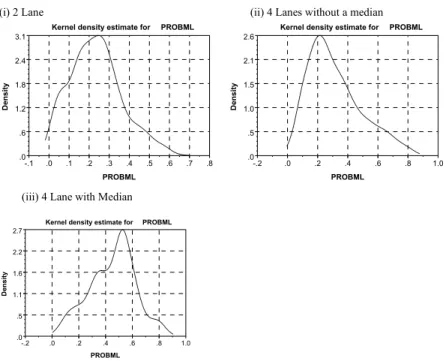
Another useful behavioral contrast is the profiles of the choice probabilities for each alternative under the MLM and LCM specifications. A Kernel density estimator is used to graph the distributions non-parametrically for mixed logit (Figure 3) and latent class logit (Figure 4).

(i) 2 Lane (ii) 4 Lanes without a median

Kernel density estimate for PROBML

PROBML .6 1.2 1.8 2.4 3.1 .0 .0 .1 .2 .3 .4 .5 .6 .7 .8 -.1 De n sit y

Kernel density estimate for PROBML

PROBML .5 1.0 1.5 2.1 2.6 .0 .0 .2 .4 .6 .8 1.0 -.2 De n sit y

(iii) 4 Lane with Median

Kernel density estimate for PROBML

PROBML .5 1.1 1.6 2.2 2.7 .0 .0 .2 .4 .6 .8 1.0 -.2 De n sit y

Figure 3 Kernel Densities for Choice Probabilities for the Mixed Logit (Triangular Distribution)

(i) 2 Lane (ii) 4 Lane without median

Kernel density estimate for PROBLCM

PROBLCM .8 1.5 2.3 3.1 3.9 .0 .0 .2 .4 .6 .8 1.0 -.2 Densi ty

Kernel density estimate for PROBLCM

PROBLCM .4 .8 1.2 1.7 2.1 .0 .0 .2 .4 .6 .8 1.0 -.2 De n s it y

(iii) 4 Lane with Median

Kernel density estimate for PROBLCM

PROBLCM .3 .6 .9 1.2 1.5 .0 .0 .2 .4 .6 .8 1.0 1.2 -.2 Densi ty

An assessment of figures 3 and 4 suggest that the choice probability range is greater for the latent class model than for mixed logit; however the differences appear visually not to be substantial with the possible exception of 2 lane. However the shapes of the distributions are markedly different with 4 lane without a median displaying the greatest similarity. To illuminate the differences we propose two profiles: (a) a plot of the choice probabilities for mixed logit and latent class logit for each respondent’s choice set (Figure 5), and (b) a graphing of the ratio of the equivalent choice probabilities for each respondent choice set (Figure 6).

The graphs in Figure 5 show the relationship between the choice probabilities under MLM and LCM most vividly. The 4-lane choice probabilities map most closely, especially 4 lanes without a median which are tight around the 45 degree line. The OLS models accompanying the graphs show that over 77% of the variance associated with the choice probability for LCM for 4 lane without a median explains the choice probability for mixed logit. In contrast only 35.7% of the variance is explained for 2 lanes. From this evidence we can conclude that the relationship between the predicted choice probabilities under the mixed logit model (and a constrained triangular distribution on the random parameters) and the latent class model (for 3 latent classes) is relatively weak at the individual respondent level. At the aggregate choice shares level for the sampled population, the respective shares respectively for 2 lane, 4 lane with and without a median are (MLM: .233, .315, .451) and (LCM: .317, .270, .412).

(i) 2 Lane (R2 _{= 0.357) (ii) 4 Lane without median (R}2 _{= 0.775)}

Figure 5 Comparison of Probability Profiles of LCM and ML

When we take the ratio of the choice probabilities of LCM to MLM (Figure 6) we find that the distribution around 1.0 is skewed to the left for 2 lanes, and slightly to the right for 4 lanes with and without a median. The majority of the ratios lie in the 0 to 2 band. Again there is a noticeable variation around equality of choice probabilities leading us to conclude that each model is representing the choice responses quite differently for the majority of the sample. In the main, the kernel plots of these ratios suggests the broad similarity of the predictions from the two models.

(i) 2 Lane (ii) 4 Lane without median

Kernel density estimate for PROBRAT

PROBRAT .2 .5 .7 .9 1.2 .0 0 1 2 3 4 5 6 -1 Densi ty

Kernel density estimate for PROBRAT

PROBRAT .3 .5 .8 1.0 1.3 .0 0 1 2 3 4 5 -1 Density

(iii) 4 lane with median

Kernel density estimate for PROBRAT

PROBRAT .2 .4 .6 .7 .9 .0 0 1 2 3 4 5 6 -1 Density

Figure 6 Comparison of Probability Profiles of LCM and ML: Ratios

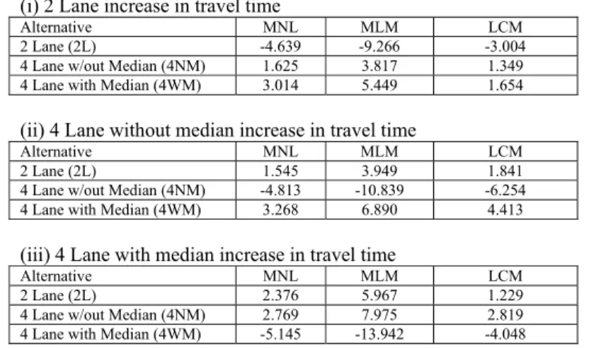
Finally, we compare the change in absolute choice shares in response to a change in the level of attributes across the sample. We have chosen a 50% increase in travel time, assessed for each alternative, one at a time. The results (in Table 4) show a greater change in absolute choice shares after full sample enumeration for mixed logit than latent class logit. As expected, this is consistent with the choice elasticity evidence in Table 3.

Table 4 Comparison of Sensitivity to 50% increase in travel time Note: The 50% increase is applied to each alternative separately.

Absolute change in choice share (i) 2 Lane increase in travel time

Alternative MNL MLM LCM

2 Lane (2L) -4.639 -9.266 -3.004 4 Lane w/out Median (4NM) 1.625 3.817 1.349 4 Lane with Median (4WM) 3.014 5.449 1.654

(ii) 4 Lane without median increase in travel time

Alternative MNL MLM LCM

2 Lane (2L) 1.545 3.949 1.841 4 Lane w/out Median (4NM) -4.813 -10.839 -6.254 4 Lane with Median (4WM) 3.268 6.890 4.413

(iii) 4 Lane with median increase in travel time

Alternative MNL MLM LCM

2 Lane (2L) 2.376 5.967 1.229 4 Lane w/out Median (4NM) 2.769 7.975 2.819 4 Lane with Median (4WM) -5.145 -13.942 -4.048

5. Conclusions

This paper has contrasted a mixed logit model with a latent class logit model. The objective was to seek some understanding of the relative merits of both modeling strategies, each regarded as an advanced interpretation of discrete choice models. Both models offer alternative ways of capturing unobserved heterogeneity and other potential sources of variability in unobserved sources of utility. Like any empirical evidence, our judgments are conditioned on a single data set’s performance under alternative behavioral assumptions.

It might be desirable to decide that one approach is unambiguously preferred to the other, but this is not possible. Each has its own merits. The latent class model has the virtue of being a semiparametric specification, which frees the analyst from possibly strong or unwarranted distributional assumptions about individual heterogeneity. The mixed logit model, while fully parametric, is sufficiently flexible that it provides the modeler a tremendous range within which to specify individual, unobserved heterogeneity. To some extent, this flexibility offsets the specificity of the distributional assumptions. We do find that both models allow the analyst to harvest a rich variety of information about behavior from a panel, or repeated measures data set.

We regard the (stated choice) data set as of high quality in terms of it delivering a substantial amount of variability that can be explained by both models. Overall it is a marked statistical improvement over multinomial logit. Which model is superior on all behavioral measures of performance is inconclusive despite stronger statistical support overall for the latent class model (on this occasion). The inconclusiveness is an encouraging result since it motivates further research involving more than one specification of the choice process. Based on the empirical evidence herein, both mixed logit and latent class logit offer attractive specifications. We encourage a greater effort to compare and contrast such advanced models as one approach to searching for rules on stability in explanation and prediction.

6. References

Gourieroux, C., Monfort, A., Trognon, A. (1984) Pseudo maximum likelihood methods: applications to Poisson models, Econometrica, 52, 701-720

Gourieroux, C., and A. Monfort (1996). Simulation-Based Methods Econometric

Methods. Oxford: Oxford University Press.

Greene, W. (forthcoming 2003) Econometric Analysis, 5th ed., Prentice Hall: Englewood Cliffs.

Greene, W. (2001), “Fixed and Random Effects in Nonlinear Models,” Working Paper

EC-01-01, Stern School of Business, Department of Economics.

Heckman, J. and Singer, B. (1984) Econometric duration analysis, Journal of

Econometrics 24, 63-132.

Hensher, D.A. and Greene, W.H. (in press) Mixed logit models: state of practice and warnings for the unwary, November

Hensher, D.A. and Sullivan, C. (in press) Willingness to pay for road curviness and road type for long distance travel in New Zealand, Transportation Research E.

Louviere, J.J., Hensher, D.A. and Swait, J.F. (2000) Stated Choice Methods and

Analysis, Cambridge University Press, Cambridge.

McFadden, D. and K. Train (2000) Mixed MNL models for discrete response, Journal

of Applied Econometrics, 15, 447-470.

Nagin, D. and K. Land (1993), Age, criminal careers, and population heterogeneity: specification and estimation of a nonparametric mixed Poisson model,” Criminology, 31 93), 327-362

Roeder, K., K. Lynch and D. Nagin, “Modeling Uncertainty in Latent Class Membership: A Case Study in Criminology,” Journal of the American Statistical

Association, 94, 1999, pp. 766-776.

Swait, J. (1994) A structural equation model of latent segmentation and product choice for cross-sectional revealed preference choice data, Journal of Retail and Consumer