Semantics driven adjoints of the message passing interface

(1)

Semantics Driven Adjoints of the Message Passing Interface

Von der Fakult¨at f¨ur Mathematik, Informatik und Naturwissenschaften der RWTH

Aachen University zur Erlangung des akademischen Grades eines Doktors der

Naturwissenschaften genehmigte Dissertation

vorgelegt von

Diplom-Informatiker

Michel Schanen

aus

Luxemburg, Luxemburg

Berichter:

Univ.-Prof. Dr. rer. nat. Uwe Naumann

Univ.-Prof. Dr.-Ing. Martin B¨ucker

Tag der m¨undlichen Pr¨ufung: 24.10.2014

(2)

(3)

3.4.3 Persistent Communication . . . 43 3.5 Nondeterminism in MPI . . . 44 3.6 Collective Communication . . . 45 3.6.1 Broadcast . . . 45 3.6.2 Reduction . . . 47 3.6.3 Allreduce . . . 55 3.7 Barrier . . . 59 3.8 One-Sided Communication . . . 59 3.8.1 Fence . . . 62 3.8.2 Get . . . 62 3.8.3 Put . . . 66 3.8.4 Accumulate . . . 68

3.8.5 Passive Target Synchronization . . . 75

3.9 Guidelines for an Adjoinable MPI Code . . . 76

4 Adjoint MPI Library 77 4.1 Usability . . . 77

4.2 Adjoint MPI Implementation . . . 79

4.2.1 Portable Data Reversal Mechanism . . . 79

4.2.2 Nonblocking Point-to-Point Communication . . . 81

4.2.3 Collective Reduction Communication . . . 82

4.3 Second-Order and Higher Adjoint Communication . . . 83

4.3.1 Tangent-Linear Communication . . . 84

4.3.2 Second-Order Code withdcc . . . 85

4.3.3 Higher Adjoints . . . 89

5 Applications 91 5.1 Hardware Setup . . . 91

5.2 Overview: Heat Equation . . . 92

5.3 Use Case: NAG Fortran Compiler and Sisyphe . . . 95

5.3.1 AD-enabled NAG Fortran Compiler (CompAD) . . . 96

5.3.2 AMPI and CompAD . . . 96

5.3.3 Sisyphe . . . 99

5.3.4 Results . . . 102

5.4 Use Case:dco/c++and PETSc . . . 104

5.4.1 Integration intodco/c++ . . . 104

5.4.2 Motivation . . . 107

5.4.3 PETSc . . . 108

5.4.4 Continuous Nonlinear Solvers . . . 109

5.4.5 Results . . . 109

6 Discussion 113

7 Summary and Conclusion 115

(5)

CONTENTS 5

A User Documentation 119

A.1 AD Tool Developer . . . 120

A.2 AD Tool User . . . 121

A.2.1 Installation . . . 121 A.2.2 Usage . . . 122 A.2.3 Fortran . . . 122 A.2.4 Example . . . 123 B Developer Documentation 127 Bibliography 157 Index 163

(6)

(7)

Abstract

Access to correct derivative information is crucial in numerical simulations and optimization. While finite differences easily provide derivative approximations through perturbing a function’s inputs, the adjoint derivative model is the only way of acquiring a function’s gradient both at machine precision and at the same time complexity as the initial function evaluation. However, the adjoint model implies a complete data flow reversal of an executed program. The same implication holds for the Message Passing Interface (MPI) of a parallel implementation. Every communication pattern has to be reversed when the adjoint model is applied.

This work establishes a framework for the semantic analysis of MPI communication patterns. It formulates a semantic driven generation of adjoint patterns of the corresponding original patterns. The MPI standard defines the semantics of every MPI communication in English language. A more abstract representation of the MPI semantics is extracted and used in order to apply the logic of Algorithmic Differentiation (AD). Based on these adjoint pattern representations a generic adjoint MPI library is im-plemented that may be used semi-automatically with any AD tool. Moreover, the runtime expectation of such an implementation on current cluster systems is analyzed. The outcome is tested with two software packages used in numerical science. One is the Portable Extensible Toolkit for Scientific computation (PETSc). It is currently one of the most robust frameworks for parallel linear and nonlinear solvers that exist. The other one is Sisyphe, a sediment transport simulation software used in the context of the fluid solver OpenTELEMAC.

(8)

(9)

Acknowledgment

I am very thankful to the following people without whom this work would have been bound for failure. • To Jan Riehme who, while integrating AMPI into Sisyphe, taught me a lot about programming in

numerical science. From simple bash scripts to general approaches (result analysis, code style,. . . ), he increased my productivity and insight by several orders of magnitude. Unfortunately, I failed at the coupled model.

• To Laurent Hasco¨et and Jean Utke who were perhaps the only people that listened to my adjoint MPI gibberish. I thank both for dismantling my reasonings whenever I was wrong and helping me out.

• To my supervisor Uwe Naumann who always emphasized one’s strengths in doubtful times. • To Klaus Leppkes for his hacking skills.

• To all the people at the STCE for the proofreading and keeping my spirit high. Not a single dispute in all these years tells me something.

• To the Fonds National de la Recherche of Luxembourg for the financial support under grant PHD-09-145.

• And last but not least to my girlfriend Paule Apel for proofreading my work and for the support during stressful times.

(10)

(11)

Chapter 1

Introduction

1.1 Background

This dissertation was created at the Software and Tools for Computational Engineering (STCE) institute of RWTH University in Aachen. At the time of this writing the institute’s research was primarily focused on Algorithmic Differentiation (AD). Every research topic that is linked to AD or that revolves around accumulating derivatives is potentially of interest to the research unit. This work is situated at the cross section of AD and the parallel programming paradigm defined by the message-passing interface (MPI). It describes where both worlds and their models meet and emphasizes the difficulties as well as the potential gains using both numerical tools together in the scientific computing field.

AD arose from the idea that every computer program is composed of a sequence of algebraic state-ments and assignstate-ments. If one neglects the I/O operations or hardware commands, every computer pro-gram in the end models a mathematical function. For any computer or numerical scientist it is clear that this abstraction itself already bears a lot of potential problems. Looking at Figure 1.1, a sine function is implemented. In mathematics the function is defined on the continuous domain of real numbers. This domain is conveyed to the numerical world of a computer through the type of the variable. Here it is the type “double” that represents a number with double precision in C++. This abstraction ignores the fact that this variable is not actually continuous anymore, but is instead bound to the machine’s precision. Furthermore, cancellation and truncation errors arise due to the internal representation and computation of numbers inside a computer’s discrete structure. The next abstraction is actually a language property. Imperative programming languages are not translatable into mathematics and vice versa. What is the meaning of for example the equal sign ”=”? In a programming code there is the notion of memory loca-tions called ”reference by address”, whereas mathematics only deal with ”reference by name”. A variable in a program may change its location or it may be overwritten. The equal sign relates to the contents of the memory location, whereas the mathematical equal sign relates to the logical truth of a statement.

f :_R_→_R x_7→sin(x)

(a) Mathematical function

1double f(double x) { 2 x=sin(x);

3 return x; 4}

(b) Implemented abstraction

Figure 1.1: The fundamental assumption in AD

(12)

These issues will not be covered in this work and it is assumed that if any function is mathematically differentiable, the same holds for its implementation. This link between mathematics and computer code is the core idea of AD. It is its strength as well as its weakness.

In mathematics, humans are able to differentiate functions using the chain rule. The application of the chain rule is rather mechanical and does not involve any creative process. It is a task, easily described by an algorithm that is taught at high school. The differential calculus is tedious and boring, causing errors due to a slip of the pen or lacking attention. Computer algebra tools may be used to symbolically differentiate functions and relieve us humans from this ever boring task. With respect to this automatic generation, AD is the algebra tool equivalent at the source code level. The source code is manipulated in a way that it becomes the implementation of the differentiated function. Having linked mathematical functions and actual implementations and having access to enough computational power, we are today able to implement differentiation tools that apply the chain rule exactly in the same mechanical way as humans do. The development of such tools are the outcome of research in the field of AD. It assumes that if this function is continuous and partially differentiable, the same holds true for its implementation. It follows that the aforementioned computer program is differentiable as a sequence of statements by applying the chain rule to all statements in the code. Considering an implementation as a sequence of differentiable statements, we are in theory able to compute semi-automatically the gradient or Jacobian of an arbitrary code. Although the application of the chain rule is straightforward, the next question we face is about the complexity of such a computation. What is the cost of accumulating the gradient or the Jacobian compared to the original implementation? What about sparse Jacobians, gradients, conversion behaviour of the derivatives and so on?

The context when dealing with these issues is mainly in the field of large-scale numerical simulations. Currently, any large numerical code is optimized to run on computer clusters interconnected by some communication network. The de facto standard in such an abstraction of communication networks is the Message Passing Interface (MPI). This work tries to find an answer to the question whether the methods of AD may be applied to MPI communication the same way as to any sequential code.

1.2 Message Passing Paradigm Meets Algorithmic Differentiation

In parallel computing, message passing is one of the first paradigms to describe the distributed compu-tation of a task. Sequential processes communicate over a network in order to synchronize tasks. Each process has its own memory space and is only able to access information on another process through this communication network. There is no notion of shared-memory, where different processes work in the same address space. First implementations appeared during the 80s and culminated into the open Message Passing Interface (MPI) standard in 1994 [39]. The use of MPI is not restricted to any particular field in high-performance computing. However, in this work the focus is on numerical simulation science, since this is the main field of application for AD.

In the message passing paradigm data is moved by sending a message composed of a source, a sink and a value. This paradigm is used in parallel computing to model the interprocess communication that takes place on a network between connected computer nodes. The communication abstraction is based on the physical communication network between the nodes. However, this paradigm could easily be applied to the local memory of a computer. Every copy or movement of data in the memory can be modelled as a communication. But virtually all computer languages vowed for an assignment (=) operation emerging from the mathematical equal sign (=). Looking more closely at the assignment operation one sees that this operation has actually more in common with a communication of the right-hand side to the left-hand side rather than with the mathematical equal sign. For example the statementx = x+ 2in Fortran does not make any sense using the semantics of mathematics. The right-hand side and left-hand side do not have the same properties. In computer programs it actually means that first the right-hand side is

(13)

1.3. PRIOR WORK 13 evaluated and then its contents are moved (or communicated) to the left hand side. Since the assignment is rather a communication two questions need clarification. Is a communication also an assignment and in particular can the same logic that is applied to assignments in AD also be applied to communication?

1.3 Prior Work

Over the last 10-20 years AD has expanded into a separate field of research with its own community. There are regular meetings with the international conference on AD every four years and the yearly European Workshops on Automatic Differentiation. Research is split into the practical research revolving around the AD tools and theoretical research about the mathematical theory behind the methods put in into practice in AD. The community supports a website1_{where among other things the biannual meetings} as well as the publications are announced.

Exploiting parallelism has become an important subject in AD due to the ubiquity of parallelism in simulation codes. It is being approached on several levels, while the focus today is on the commonly used parallelization standards OpenMP and MPI. Moreover, adjoint computations on GPUs are also making their first entry into AD.

First, algorithms have been developed that exploit the inherent parallelism of AD. This applies for ex-ample to the tangent-linear mode, adjoint mode or vector mode. Most of these methods rely on OpenMP. For example one can exploit data dependencies of first-order and second-order tangent-linear code to compute both orders of differentiation in parallel [37, 9, 8]. Or the trace of the adjoint computation may be split among the memory of several computer nodes on a cluster system and interpreted partly in parallel.

Second, given a particular class of code that is automatically parallelizable, the method in [?] gen-erates a parallelized automatically differentiated AD code, thus combining automatic differentiation and automatic parallelization. The codes consist of matrix-matrix multiplications on a theoretical hybrid computer architecture based on arrays and trees of processing elements.

This thesis is situated at the third level of parallelization in AD where the parallelism of the original code should be conveyed to the differentiated code. The user introduces parallelism in the original code. However, the AD tool has to have the capability of differentiating the parallel statements. No tools today have a straightforward, user friendly and automatic way of differentiating any parallelism. OpenMP exploits thread based parallelism inserted through pragmas at the compiler level whereas MPI is a process based communication runtime library for parallelism at the process level. This work deals with inter process communication in MPI whereas a PhD thesis with a similar goal in OpenMP was achieved in close collaboration [16].

First attempts have been made in 1999 by automatically adjoining MPI_Send, MPI_Recv and MPI_Reducein the source code transformation tool Odyss´ee. Odyss´ee automatically reverses the send and receive as well as the sum reduction (MPI_ReducewithMPI_SUM) [15, 14]. Only in recent years AD tools have become aware of any parallelism. A solution for the tangent-linear mode has been pre-sented by using derived data types, although this is again not applied automatically [10]. TAF claims to have OpenMP and MPI support without being clear about the specifics. ADOL-C claims to have sup-port for the MPI communicationsMPI_Send,MPI_Recv,MPI_BroadcastandMPI_Reduce. In general, a substantial intervention into the original code is required [52] or the support is limited to the tangent-linear mode [55] (ADIC and ADIFOR).

Sketches have been outlined about how an AD tool should adjoin MPI with the communication re-versal being the main issue [29]. More complex patterns like nonblocking communication have been addressed in [62]. A general differentiation approach for MPI communication, especially for the ad-vanced ones like for example one-sided communication, is still missing.

(14)

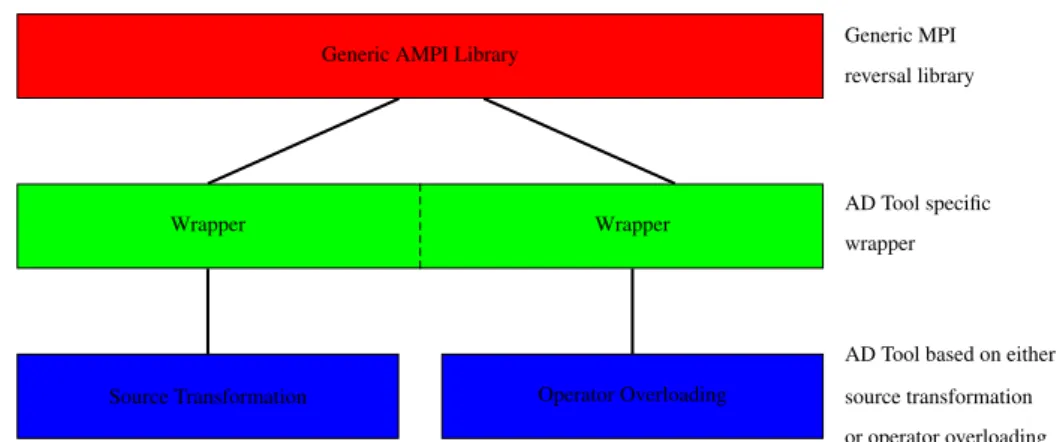
Automatically differentiating MPI is primarily driven by a joint effort of the Argonne National Lab-oratories, INRIA and our institute at the RWTH Aachen University. The first goals had been set in 2009 [62]. This is the time where this work started. The common target is a generic adjoint MPI library that may be incorporated into any AD tool in order to differentiate MPI enabled codes automatically.

1.4 Problem Statement

When applying AD to the Message-Passing Interface, whether automatically or manually, four questions need to be clarified.

• Feasibility:Does a reversal scheme exist? Is a given MPI pattern adjoinable?

• Closure: Is the adjoint communication pattern still expressible in MPI and is there a possible trade-off?

• Correctness:Is the generated adjoint MPI code correct?

• Efficiency:How do the complexities of the original and adjoint communication pattern relate? In order to prove feasibility and closure, one has first to develop an abstract framework which enables us to prove the correctness of an adjoint pattern. This abstraction is driven by the semantics of the MPI standard. The MPI standard relies for the most part on the English language as its defining language. In order to apply AD, the theoretical part of this work will be about the extraction of the semantics in a more mathematical framework. This framework allows us to prove the correctness of adjoint communication patterns that are based on heuristics. Feasibility and closure are linked to the efficiency. One has to subjectively decide whether a given code may still be considered feasible if there is a substantial decrease in efficiency. In particular, the adjoint pattern should stay in the same complexity class as the original pattern.

An adjoint MPI library is implemented for the core routines of the MPI 2.2 standard. If there exists an adjoint communication inside the MPI 2.2 standard, the adjoint generation is considered to be enclosed in MPI. However, we also require the adjoint patterns of the different classes of MPI communications (point-to-point, collective, one-sided) to be closed. Adjoining one-sided communication should for example not resort to blocking point-to-point communication.

1.5 Summary of the Results

All the classes of MPI communications in the MPI 1.1 [39] standard yield efficient adjoint communi-cation patterns including the reductionMPI_Reducewhich applies arithmetic operations on the buffer elements. The MPI 2.2 standard [40] introduces one-sided communication which includes nondetermin-istic behaviour. Nondeterminnondetermin-istic behaviour in MPI 1.1 was restricted to wildcards, WAIT_ANYand TEST_ANY. They posed no threat to the feasibility of an efficient adjoint computation because MPI comes with the necessary information to trace the nondeterministic instance of the communications. This changes with one-sided communication. It is for the first time analyzed in detail and adjoint pattern de-scriptions are discussed. The outcome is that the accumulationMPI_Accumulate, in conjunction with the product operationMPI_PROD, is the first MPI communication that is proven to be not adjoinable at a reasonable runtime cost. Especially passive target synchronization proves to be impossible to adjoin without user input. Nondeterminism proves to be at the heart of future development of adjoint MPI.

On top of the theoretical results and insights, an adjoint MPI library is designed and implemented. Its design requires reflection on the theoretical results as well as on the generic AD tool structure. The

(15)

1.5. SUMMARY OF THE RESULTS 15 implementation is then tested in Sisyphe (sediment transport simulation) and PETSc (linear and non linear parallel solver framework).

At the end, the combination of continuous and discrete adjoints seems more important than ever on current high performance computing platforms where memory is rather limited. Discrete adjoints is the straightforward application of the adjoint model at the statement level of a function’s implementation. Continuous adjoints is the implementation of the mathematically derived adjoint function of the original function. Purely discrete adjoints prove to be very hard on current cluster systems due to their large memory footprint (see Section 3.1.2), whereas continuous adjoints potentially lead to a lower memory footprint than discrete adjoints (see Section 5.4). Although this is not subject of this work, the perfor-mance of AMPI is linked to the perforperfor-mance of discrete adjoints in general. With discrete adjoints being far from trivial on cluster machines, the use case of AMPI is currently severely limited. AMPI proves to be a great tool for adjoining the distribution and combination of data that takes place around a highly optimized computational core of a numerical simulation. Whether it is suitable for fully discrete codes remains an open question.

(16)

(17)

Chapter 2

Foundations

This chapter lays out the formalism on which this work will build upon. Starting with a brief overview of MPI (Section 2.1) and AD (Section 2.2), possible technical constraints are anticipated in Section 2.3. The single assignment code (Section 2.4) from AD is then combined with the parallel formalism of the partitioned global address space (Section 2.5). To cope with the MPI semantics additional constructs are introduced in Section 2.6.

2.1 Message-Passing Interface

The first Message-Passing Interface (MPI) standard was published in November 1992 [39]. This standard was the result of a long evolution that has its roots in one of the oldest parallel computation paradigms. It tries to abstract the combination of single computers that are merged together to form a computer

cluster. At that time its unique feature was its open standard description. The standard was established

by a committee composed of various entities ranging from industry to academia. Before, a computer cluster was a black box which handles the parallelization on a specialized hardware opaque to the user, only accessible through a special programming interface. This is still the case for some specialized memory systems today. It is hard to find a common abstraction that matches all the shared-memory systems due to their highly specialized hardware. A code written in an abstract language may run efficiently on one system, while being a complete failure on another system. General open

shared-CPU Mem. CPU Mem. CPU Mem. CPU Mem. CPU Mem. CPU Mem. Node: Network: CPU Mem.

Figure 2.1: Hardware abstraction in MPI

(18)

memory standards only appeared very recently (e.g. OpenMP 1997) .

For distributed memory systems the abstraction is far easier, even if the hardware is highly special-ized. Each single computer system inside the cluster is anodethat is connected to other nodes through a

network(see Figure 2.1). Each running process has access to all the hardware of a single node [53, 22]. In

general the hardware is described by one CPU and one memory address space. In order for one process to access memory of another node, the data has to be communicated through the network. This is achieved by the dual operation of sending and receiving messages. First message passing libraries were mostly tailored to specific hardware and tied to a specific system. Soon it became apparent that the assumption of having nodes and a network was common to all the implementations. A common interface was finally defined and published in Fortran and C in 1992. MPI defines some common operations that should be executable on the computer cluster. The simplest one is a send or receive. Other operations are for exam-ple collective operations like the gathering or scattering of data. MPI cannot know how your hardware and your network with its topology may efficiently execute these operations. Hence, there is no reference implementation. Anyone may implement an MPI library while strictly adhering to the interface standard, so vendors have still to develop specialized libraries. However, the developer costs dropped dramatically, since any MPI code is portable to any cluster that supports the standard without any code amendments. This huge gain in portability had no disadvantage to other non standardized libraries and finally meant a huge success for MPI. Today, MPI has received widespread acceptance in the high performance com-putation community and has become the de facto standard in high performance computing. There are a wide range of MPI libraries, some for general purpose while other implementations only run on a specific hardware of one cluster type. All TOP 500 clusters support the MPI interface, meaning that any MPI enabled code runs on any of these TOP 500 clusters as well as potentially on any consumer laptop or even embedded devices.

2.2 Algorithmic Differentiation

AD revolves around the computation of derivatives using the chain rule of differential calculus. Algo-rithms are developed that exploit the property of the chain rule. The user is relieved from the effort of mechanically differentiating code (see motivation in Section 1.1). The error-proneness of handwritten differentiated code may drive costs higher than any budget could ever cover. One advantage of AD is indeed a considerably reduced maintenance cost of the adjoint code.

What algorithms to use in the end is a vast field of research. Symbolic differentiation has its beginning in 1953 [23]; the time around which computers were powerful enough to generate code in assembler. In 1976 the term “Automatic Differentiation” made its first appearance in the context of Fortran. Kedem observed that any subroutinefooin Fortran could be transformed into a subroutinefoo0_{that computes} the derivatives of subroutinefoo[32]. The final spark was in the 80s with Rall in 1981 [54] and Griewank around 1989 [18], making AD an independent research field.

In numerical simulation and optimization access to exact derivative information is crucial for the performance and correctness of the underlying simulation [30]. In AD it is assumed that every numerical code may be treated as a multivariate vector functiony=F(x) :_Rn

→Rmwithxbeing the inputs and

ybeing the outputs. Since any code may be interpreted as an input code for AD, the output code of an AD tool is again valid input for an (another) AD tool. This recursive reapplication is a way of applying second order or higher derivative models.

Extracting derivative information amounts to extracting the level of dependence between theninputs

xand themoutputsy. The mathematical theory behind it, is the differential calculus denoted by partial derivatives _dxdy. Its main field of application in numerical science is optimization [13] and sensitivities, ranging from simple non-linear functions to iterative solvers or sensitivities in shallow water simulations [56]. There is no limitation to the extend of the code base as long as the AD tool is able to differentiate

(19)

2.2. ALGORITHMIC DIFFERENTIATION 19 the code at the statement level for a given programming language. The needed derivative information may vary from single derivative values or gradients up to entire Jacobians or Hessians.

The accumulation of derivative information yields subproblems in theoretical computer science. For single derivatives there are two differentiation models, tangent-linear and adjoint, with different runtime behaviour (see Section 2.2.3 and Section 2.2.4). Another method, called edge or vertex elimination, may be used for example in the Jacobian accumulation where all the entries of the Jacobian are computed. Finding the minimal number of floating point operations needed to accumulate the entire Jacobian has been proven to be NP-complete [42]. This last method of finding the minimal number of operations (see [21] on Accumulation by Vertex-Elimination) uses edge or vertex elimination on the directed acyclic graphs in order to extract the differentiated code. This method is not subject of this work.

2.2.1 Textbook Example

The following problem serves as a textbook example of an AD application the way it commonly occurs in simulation science. It is structurally a data assimilation problem with, for the purpose of simplification, a basic cost function. Data assimilation [31] problems with scalar cost functions emphasize the benefits of the adjoint model which is not available while using finite differences. Furthermore, it is easily decom-posable into subproblems and thus embarrassingly parallel (MPI). Our code where AD is applied consists primarily of three parts:

• subproblem • cost function

• optimization algorithm

Without the loss of generality thesubproblemor simulation model is assumed to be a multivariate functionuthat computesmvalues with respect to inputsx_∈ _Rn_{and some undetermined or unknown}

parametersp_∈_Rl_._p_{may be composed of model parameters or may just consist of the initial values of}

u. For some inputx,oobserved valuesuob₍_x₎_{are measured through experiments in the real world. The}

discrepancy between computed valuesui(xi,p) and observed valuesuobi (xi)for some input valuesxiis

the simulation error and should be0with an ideal simulation model. For a given number of observations o, this error is summed up as acost function

J(p) =

o

X

i=1

(ui(xi,p)−uobi (xi))2 .

which is assumed to be only dependent on the parameterspfor a given number of observations and input valuesxi. In a data assimilation problem like for example 3D-Var [31] the cost functionJ may be far

more complex. For some observed valuesuob

i we try to minimizeJ(p)through adapting the simulated

valuesuiby optimizing the values ofp.

For the minimization ofJwe use theoptimization algorithmSteepest Descent or Gradient Descent. It is a first-order derivative based optimization algorithm that is guaranteed to converge to a local minimum.

pk+1=pk−α∇J(pk)

It iteratively minimizes J(pk) by computing a new valuepk+1 through the subtraction of ∇J(pk).

Usually, the scaling valueαis determined through a line search algorithm. More details and numerical properties of this method are described in [51].

In each optimization step we want to access derivative information that describes the dependence of the l parameter inputs with respect to the single outputJ. Whether first-, second- or higher-order

(20)

derivatives are needed is up to the optimization method (here Steepest Descent). This example will serve as the prime motivation for the adjoint model and should illustrate why in the end, adjoints in an MPI setting are indeed important. Both case studies, PETSc in Section 5.4 and Sisyphe in Section 5.3.3, are motivated by a similar setting.

In the next sections each of the different mathematical methods of accumulating derivatives is pre-sented and how these methods relate to this example. In particular, the focus is on the implications for MPI enabled code. For each method we consider a multivariate vector functionRn → Rm with

y=F(x). FunctionF hasninputsandmoutputs. We relate runtime complexity of the differentiated code with respect to theninputs andmoutputs.

2.2.2 Finite Differences

Finite differences approximation is perhaps the most widely used way of accumulating derivative infor-mation. It avoids the handwriting that results from the application of the chain rule and uses the original code to compute derivatives. It relies on the finite differences quotient to compute approximated partials ∇xiF

∇xiF(x)≈

F(x+h·ei)−F(x)

h ,

for the Cartesian basis vectorei∈Rnand the inputsx∈Rn. It is a direct consequence of the definition of the derivative, first described by Newton [50] and Leibniz [34]. To accumulate the entire Jacobian of our functionF, we have to perturb each of the inputs and therefore rerun the entire codentimes. Finally the unperturbed values have to be computed once. Thus the complexity amounts to_O(n)_·cost(F). However, the finite difference quotient is only an approximation of the partial derivatives.

The reason why finite differences are being so widely used is that this method is particularly easy to implement. The original code of the functionF may be used unaltered. This is especially true for any library calls like MPI where no special treatment is necessary. The code is just run once for each perturbed input and once with no perturbation at all. The approximation error represents a major drawback for codes that implement highly nonlinear systems, resulting in truncation and cancellation errors or simply providing wrong results. By applying the Taylor expansion to the second-order centered finite differences quotient, a machine precision induced approximation error of

h2 is derived, withbeing the rounding error. An additional drawback is that the runtime is always dependent on the number of inputsn. Finite differences do not provide a mode that shifts the runtime dependence from the inputs to the outputs. As we will later see, AD provides such a mode. On the upside, one may observe in practice a regularizing effect of finite differences when using a step based algorithm. Where AD may lead to non convergence, finite differences may succeed due to its smoothing effect.

MPI

As for any library, using finite differences is straightforward and no special treatment is necessary for MPI enabled codes. The underlying parallelization is used unaltered and the performance should be similar to the original code while it has to be executedn+ 1times, once for each direction and once for the function evaluation.

2.2.3 Tangent-Linear Model

The tangent-linear model is one of the two models in AD. Its advantage over the finite difference quotient is that it yields derivatives with machine precision. It essentially comes down to symbolic differentiation at a statement level in our code ofF. The original code ofF withxbeing the inputs andythe outputs

(21)

2.2. ALGORITHMIC DIFFERENTIATION 21 is transformed into the tangent-linear code manually or through an AD tool. All the details will not be provided, because the focus is on the consequences for an MPI enabled code. The implementation in tangent-linear modeFof a functionf using the tangent-linear model is defined by

F x↓,y ↓ AD −→F(1) x↓, ↓ x(1),y ↓ ,y(1) ↓ , where y(1)=_∇f(x)_·x(1) and y=f(x) ,

and computes the directional derivativey(1)of the outputsywith respect to the inputsx. In the tangent-linear model the input direction x(1) _is _seeded _{whereas the derivative values in the outputs} _y(1) _are

harvested. For an entire Jacobian accumulation the model has to be runntimes while seeding one of the

nCartesian basis vectors. So we end up with the same runtime complexity of_O(n)_·cost(F)as finite differences, while the constant factor due to the overhead of the implementation is obviously higher. In addition to the original function values, the tangents have to be evaluated which are more expensive than the values. A remedy for this would be the vector mode, where all thentangents could be propagated at once, but with only a single function evaluation. However, in practice vector mode may potentially increase cache misses.

MPI

The application of the tangent-linear model in MPI enabled code implies a doubling of the amount of communication. For each valuex, an additional tangent-linear componentx(1)_{has to be communicated.} The data flow and communication patterns are preserved. However, the data that is communicated under-goes a type change. Each activated variable in the original is assumed to be either of typeMPI_DOUBLE orMPI_FLOAT. Therefore, the idea is to define a new derived data type consisting of twoMPI_DOUBLE s or twoMPI_FLOATs. Additionally, the missing basic MPI operations for the reductions of the newly created type have to be implemented. As an alternative to a new derived data type one may resort to communicationshadowingby doubling the amount of communication calls; one communication for val-ues and one for the tangents (see Section 4.3.1). The implementation of a tangent-linear MPI has been achieved as a side project of adjoint MPI.

2.2.4 Adjoint Model

F x↓,y ↓ AD −→F(1) ↓ x,x(1)↓ ↓ ,y ↓ ,y↓(1) , where y=f(x) and x(1)=x(1)+∇f(x)|·y(1) . (2.1)

Exploiting the associativity of the chain rule of derivative calculus leads us to the adjoint model of dif-ferentiation depicted in Equation (2.1) [45], where the adjoint model of the functionf is given by the implementationF using an AD tool in the adjoint mode. It incrementsadjointsx(1) ∈Rnof the inputs

x_∈_Rn _{for some given adjoints}_y

(1)∈Rmof the outputsy∈Rm. With the adjoint model we are able to compute gradients with respect to some outputyiby settingyto thei-th Cartesian basis vector ofRm. The main benefit of adjoint code is its runtime dependence on the number ofmoutputs as opposed to the inputs with the tangent-linear model or finite-differences. Each Cartesian basis vector has to be setm

(22)

times for a Jacobian accumulation. In each run, one gradient of one outputyiwith respect to all inputsx

is computed. This is a huge gain for gradient based methods becausem= 1.

The adjointsx(1) of the inputsxare computed with respect to the adjointsy(1) of the outputs y. Hence, the adjoint implementation is split into two sections; theforward sectionand thereverse section. In the forward section the values are evaluated in the same order as in the original program. In the reverse section the adjoints are computed in the reverse order of the original program. For the adjointsx(1)of statements that involve non-linear functions, access to the values ofxis required for the computation of_∇F(x). This implies a complete data flow reversal programs with non-linear functionsF. This is discussed later in more detail in Section 2.4. As the available memory is a hard limit, one can use check-points in order to recompute the values ofx, gaining memory efficiency but losing runtime performance. The optimal trade-off between memory efficiency and runtime performance for a given memory bound has been proven to be NP-complete [43] in the context of call tree reversal. But even considering a given code as a DAG, it has been proven NP-complete to generate a reversal scheme through edge elimination with a minimal number of operations [44].

MPI The data flow reversal imposed by the adjoint model implies a communication reversal for all MPI calls. In the forward section the values are communicated while in the reverse section the adjoints need to be passed in reverse order. Besides this theoretical requirement, there are also practical consequences for adjoints when they are computed on MPI distributed systems, in particular the memory wall that is discussed in Section 3.1.2.

2.3 Technical Considerations

This section is directed at AD tool developers. It is helpful to be familiar with the technical details of at least one AD tool. An application of an AD tool on a code is calledactivation. Operations or data structures linked to the derivative computation are calledactive. A brief overview of the different classes of AD tools is presented with certain common traits that form a categorization. These categories should be kept in mind for later as they have consequences for the handling and the structure of the active data types with regard to MPI. All categories influence each other. For example a source transformation tool tends to rely on associating by name whereas operator overloading tools tend to use association by address.

2.3.1 Source Transformation versus Operator Overloading

The first classification of an AD tool relates to the technique that is used to semantically transform the pro-gram from computing function values to computing derivatives (ADIFOR [7], Tapenade [24], OpenAD [63]). The most portable and generic method is source transformation. The source code is transformed during a compilation process by essentially replacing the compiler front end. Instead of generating only the function values, the desired differentiation model is applied to the original code. The output may be an intermediate code that is read by the back end of the compiler or the output may be again source code. The other technique targets the very instance of a program execution at runtime (FadBad [5], ADOL-C [19], TaDiff [6], NAGWare Fortran ADOL-Compiler [48], dco [58]). ADOL-Changing a program semantically is attained through changing the variable type. Overloaded operators then operate on this new variable type according to the differentiation model. Of course, the underlying programming language has to support overloading of functions and operators.

(23)

2.3. TECHNICAL CONSIDERATIONS 23

2.3.2 Association by Name versus Association by Address

Before the compilation process a variable is generally associated by its name. There is no notion of data locality. By augmenting the code with statements that compute derivatives, the desired differentiation model is applied with respect to a variable’s name.

Listing 2.1: ”Code augmentation relying on association by name”

1 // Original code 2 w=u*v;

3 // Augmented code 4 w=u*v;

5 dw=du*v+dv*u;

In the adjoint model, required values that are overwritten have to be saved for example onto a stack. The stack pushes variables through their name.

The other option is to refer to data locality and apply the differentiation model to the contents of data. This is commonly a direct consequence of overloading tools, which introduce a new type and overloaded operators. Each time an operation is executed, the result together with a link to its arguments are saved on a trace or tape. The chain rule is not based on the variable names but on their locations on the tape. Hence, this is called association by address.

2.3.3 Contiguous versus Interleaved Memory Layout

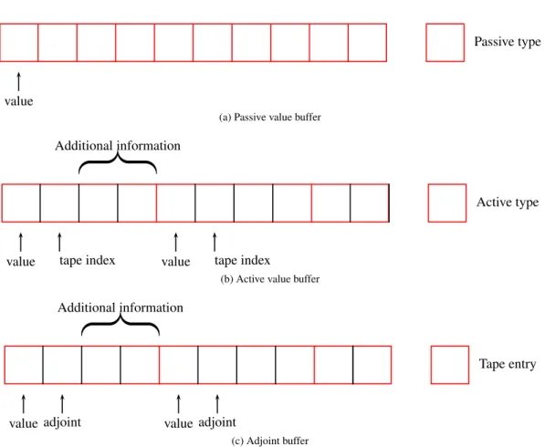
A structural difference between the tools is their memory layout (see Figure 2.2). Depending on the implementation, values or adjoints may reside in a contiguous memory space with no disparity. Source transformation tools tend to have a contiguous layout, since they probably do not change the type of the variables. Instead, they just add additional adjoint variables. Operator overloading tools on the other hand have to introduce an active type. This active type is probably different from the passive type. So we have to deal with interleaved memory if the values in the active type or the adjoints on the tape have to be accessed.

Note that this is only a rule of thumb. One could imagine a source transformation tool with interleaved types for example when storing additional information inside the variables, thus changing their type. And there exist operator overloading tools like ADOL-C [19] that force a contiguous memory layout for the values and the adjoints for some technical reasons.

2.3.4 Implications for MPI

The association by name versus association by address have both no direct consequence for an adjoint MPI code. MPI selects data to be communicated via a buffer address. Thus, the minimum requirement for writing such code is that a source transformation tool handles pointers (C) or arrays (Fortran).

The memory layout however has big implications for an adjoint MPI code. MPI only uses pointers or arrays to access the data. There is no built in support for disparities except for special communications e.g. MPI_Gather/MPI_Scatter. There are two choices. Either the entire active and adjoint type is communicated with all the additional information that is stored beyond the value and the adjoint. This may lead to clashes and is not guaranteed to work. The other way is to copy the values and adjoints in the active types into a continuous buffer that is then communicated. So when dealing with interleaved data types there is a trade off. When requiring zero copy, the interleaved types have to be converted to contiguous storage by the AD tool. A generic interface that is compatible with all AD tools leads to an additional copying of the data.

(24)

value

Passive type

(a) Passive value buffer

value tape index value tape index Additional information

Active type

(b) Active value buffer

value adjoint value adjoint Additional information

Tape entry

(c) Adjoint buffer

Figure 2.2: Non contiguous memory access

2.4 Single Assignment Code

Without the loss of generality, it is assumed that every statement that does not involve MPI amounts to an assignment. It follows that the entire code is decomposed as follows into a sequence of single assignments called Single Assignment Code (SAC) [45]:

forj=n+ 1, . . . , n+p+m vj=ϕj(vi)i≺j .

(2.2)

wherei ≺ j denotes a direct dependence of vj onvi. The result of each functionϕj is assigned to a

unique auxiliary variablevj.The n independent inputsxi = vi,for i = 1, . . . , n, are mapped onto

mdependent outputsyj = vn+p+j,forj = 1, . . . , m,and involve the computation of the values ofp

intermediate variablesvk,fork=n+ 1, . . . , n+p.The functionsϕj amount to the intrinsic functions

or operators of a programming language. Being able to differentiate every intrinsic function and operator allows us to differentiate arbitrary code written in a given programming language.

Applying the tangent-linear or adjoint model (see Section 2.2.4 and Section 2.2.3) leads us to the tangent-linear code generation

(25)

2.4. SINGLE ASSIGNMENT CODE 25 forj=n+ 1, . . . , n+p+m vj(1)= X i≺j ∂ϕj ∂vi · vi(1) .

or the generation of adjoint code

forj=n+p+m, . . . , n+ 1 (v(1)_i)i≺j =v(1)_j· _∂ϕ j(vi)i≺j ∂vk k≺j .

of arbitrary SAC as stated in [45]. Notice that in the SAC the incremental adjoint model is not used. This avoids the issue of nullification of the adjoints, which is explained in the next section.

Extending the MPI interface to the SAC notation would allow us to handle the MPI communication in a mathematical consistent way and apply both AD models seamlessly. The missing element is an ab-straction of the MPI semantics that allows us to transform MPI calls into a SAC. This requires a mapping of all MPI functions onto intrinsic mathematical functions with inputs and outputs. Having an abstract representation of the semantics of the MPI communication would then allow us to apply the adjoint model seamlessly.

2.4.1 Nullification of the Adjoints

In a SAC, as described in the last section, every intermediate variablevjis used once. This is generally

not the case in real code as variables are allowed to be used multiple times. Here is an example written in SAC but with the variablev0being used twice to store a value. Once in the statementv0=xand again in statementv0=v1. Although the valuey = 2x= 6is computed, the adjoints are wrong if they are not appropriately reset to0. 1// Forward section 2x=3; 3v0=x; 4v1=v0+v0; 5v0=v1; 6y=v0;

7// Reverse section without nullification 8a1_y=1 // seeding

9a1_v0+=a1_y; // =1 10a1_v1+=a1_v0; // =1 11a1_v0+=(1+1)*a1_v1;

12a1_x+=a1_v0; // =3, wrong!

13// Reverse section with nullification 14a1_y=0; a1_x=0; a1_v0=0 ; a1_v1=0; 15a1_y=1; // seeding 16a1_v0+=a1_y; 17a1_y=0; 18a1_v1+=a1_v0; 19a1_v0=0; 20a1_v0+=(1+1)*a1_v1; // =2 21a1_v1=0;

(26)

22a1_x+=a1_v0; // =2, correct 23a1_v0=0

Listing 2.2: Multiple variable access

In Listing 2.2 two times3is computed. Firstxis set to3(line 2) and then assigned tov0(line 3). v1is computed by the sumv0+v0(line 4). v1is assigned to v0(line 5), which is then the second time a value is assigned tov0. And last,v0is assigned to the output variabley(line 6). In the reverse want to compute the derivative ofywith respect toxaccording to the adjoint model (see Section 2.2.4). Therefore,a1_y is set to one (seeding) in line 8. The incremental adjoint model is applied to each statement and we end up with a wrong gradient of3instead of2. This is due to the missing nullification of the adjoints, in particular ofa1_v0before it is incremented a second time in line 11 after having been incremented in line 9. The conservative approach is to set every adjoint to0after its contribution is used in an incremental update. There is more on this subject in the book [45]. Moreover, due to the increment, it has to be guaranteed that every adjoint is set to0at the beginning of the reverse section (line 14). The required nullification amounts to an additional zero assignment in the SAC:

forj =n+p+m, . . . , n+ 1 (v(1)_i)i≺j += v(1)_j· _∂ϕ j(vi)i≺j ∂vk k≺j , (2.3) v(1)_j= 0 .

In this work we take the conservative approach and assume that every adjoint has to be set to0after it has been used in an incremental update. This nullification has to take place before the next increment.

2.5 Partitioned Global Address Space

Partitioned Global Address Space (PGAS) serves as an abstraction formalism to convey MPI semantics to the SAC notation in AD. PGAS is a rather new formalism in parallel computing driven by the development of the PGAS language Unified Parallel C (UPC) in the late 90s [11]. It unites the distributed memory spaces that belong to a specific process by associating each memory location or variable with the process rank. This is usually achieved by prefixing a variable with the rank of the process it belongs to. The distributed memory space is thus modelled as a shared memory space with non uniform memory access. Each process has only access to the local variables. For a process to access a remote memory location, it has first to transfer a variable to the local address space. This is modelled through an assignment of a remote memory location to a local memory location (e.g. 1.x = 0.x). An assignment with different memory locality on the left-hand and right-hand side has the same properties as a communication of variables.

In practice, PGAS has never gained widespread traction. It is easy to write PGAS code, however it is hard to make it perform well in a generic setting. There has to be either an offline or online pattern analysis, otherwise statements only model single sends and receives. More complex patterns like a reduc-tion have to be detected by the system or reintroduced through workshare constructs similar to OpenMP. However, modelling distributed memory architectures using PGAS proves to be extremely powerful in a theoretical analysis. In particular it has been utilized to prove the correctness of nonblocking adjoint message passing programs [46].

1...

2int rank=0;

(27)

2.6. MPI EXTENDED SAC 27

4double x=(double) rank;

5MPI_Bcast(&x,1,MPI_DOUBLE,0,MPI_COMM_WORLD); 6...

Listing 2.3: ’MPI code’

First we want to illustrate how the distributed memory in an MPI setting is transformed into PGAS. In Listing 2.3 we have an MPI code where the rank is determined usingMPI_Comm_rank. The rank is then assigned to a double precision variablex. The followingMPI_Bcastdistributes the value ofxon process 0 to all the other processes. To transform this code into PGAS, the name space of all the variables is changed. Every variable is prepended with an integer representing the rank of the process the variable is currently allocated on and followed by a separating dot ’.’. This prefix is unique and unambiguous in all MPI supported languages (Fortran and C) since their syntax states that no variable’s name is allowed to start with an integer.

1...

2int r.rank=0;

3MPI_Comm_rank(MPI_COMM_WORLD,&r.rank); 4double r.x=(double) r.rank;

5// Broadcast in PGAS here 6...

Listing 2.4: ’PGAS code for process r’

Following this straightforward search and prepend logic, the code of Listing 2.3 is then transformed into Listing 2.4, while omitting theMPI_Bcastfor the time being. At each occurrence of the variablesxand rank, they are replaced byr.xandr.rank. The drawback of this transformation to PGAS is that it models a particular instance of a parallel execution. Each process has its own instance. Fortunately, MPI is very clear on the specific behaviour of a communication. For the broadcast it distinguishes between the root rprocess and the rest of the processes; being a master/slave setup. The standard leaves little room for interpretation or nondeterminism, hence the order of the PGAS statements is very clear, but not unique. A PGAS single assignment code has to be found that is an abstraction of all the original MPI code instances and that yields the correct adjoints when it is differentiated. There are other ingredients beside the variable prefix that will be addressed in the next section.

2.6 MPI Extended SAC

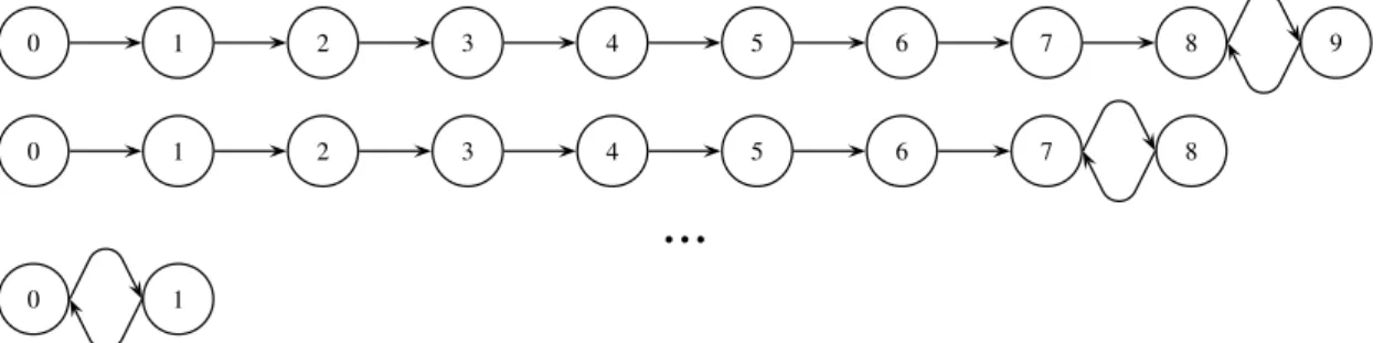
for(int i=0;i<n;i++) i.x=0.x;

(a) PGAS

for(int i=n-1;i>=0;i--) 0.x+=i.x;

(b) Adjoint PGAS

Figure 2.3:MPI_Bcastin PGAS

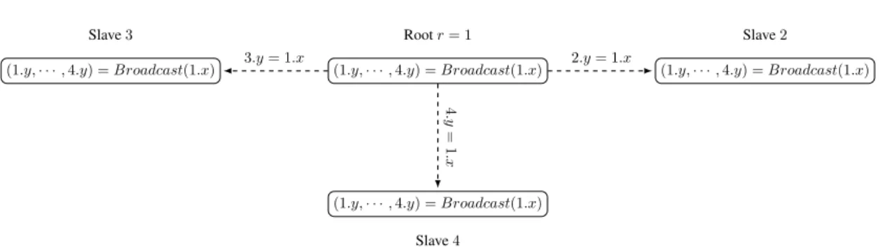
The MPI induced PGAS code described in the previous and in this section will be differentiable and allows us to apply AD and use all the logic that may be used for any sequential code. In Listing 2.4 there are single assignments where the differentiation models may be applied to. The only missing element are MPI calls like theMPI_Bcastwhich was left out in the previous section. The standard explicitly describes in detail what the input and the output of anMPI_Bcastshould be. The root variabler.xis broadcast to all the other processes inside the MPI communicator (discarded for simplification purposes). For instance, due to semantical analysis, we may generate the PGAS code presented in Figure 2.3a that corresponds to anMPI_Bcast. By interpreting the semantics of MPI any runtime instance of an MPI

(28)

enabled code is transformable into a PGAS extended SAC. The communicated messages in MPI are reduced to assignments, while the communication pattern is imitated by control flow constructs. The link between MPI and AD is established. Figure 2.3b corresponds to the adjoint statement in PGAS of Figure 2.3a.

Every statement in the PGAS extended SAC is an assignment. A local statement only involves an assignment of variables from the same process whereas an MPI call involves at least two variables of distinct process origin. Every statement in PGAS is defined by extending the SAC as follows

forj=n+ 1, . . . , n+p+m rp.vj =ϕj(rl.vi)i≺j ,

whererp andrlare the rank of the participating processes pand0 ≤ l < numprocs. This way we

are able to map any MPI enabled SAC onto a PGAS SAC, thus allowing us to differentiate the resulting code using the tangent-linear or adjoint model. One difference between a SAC derived from a sequential program and a PGAS extended SAC derived from an MPI enabled code is the potential nondeterministic behaviour introduced in parallel code execution. The SAC for an instance of a sequential program is unique and only dependent on parameters that were set before the execution started. In parallel com-putation there are nondeterministic effects that yield different PGAS extended SACs. The ordering of the statements is not unique for example in case of two independent local statements on two different processes. Fortunately, MPI forces some statement order through implicit or explicit synchronization.

There are three issues that need to be addressed to make the semantic extraction of a PGAS extended SAC of MPI enabled code a generic tool:

1. Variable operations

2. Concurrency and nondeterminism 3. Variable locks

The variable operations inside communications are equivalent to standard SAC operations. So we are left with 2 and 3.

Communication is equivalent to an assignment in PGAS. However, MPI calls should be treated as intrinsic functions unrelated to an assignment. This has certain benefits for high level MPI calls or for one-sided communication. The MPI communication ought to be mapped onto mathematical functions with input, outputs and inherent semantics. The semantics may dictate some additional constraints on variable access (non-blocking, one-sided) or operate on the variables (reduction). These semantics are directly derived from the MPI standard. It is a mathematical interpretation, since the standard itself is primarily written in prose. Any MPI code that does not fulfill the semantics interpretation is not a valid MPI code and thus potentially not adjoinable.

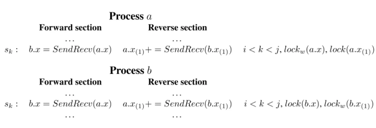
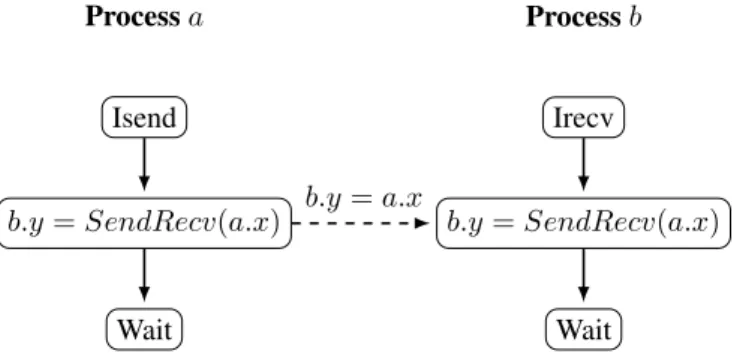
The code in Figure 2.4 is the extended SAC of a nonblocking Send/Receive pair, while omitting the nullification of the adjoints. Data is being sent from processato processb. The function that transfers the data is the intrinsic functionSendRecv. It is executed on both processes with the receiving and sending ranks defined through the PGAS notation. b.x is the output on the left-hand side whereas a.xis the function argument and serves as the input to theSendRecv. Without additional information, this would correspond to a blocking send and receive. The information on the right is explained in the following two sections. This first isorder of the statementsthrough the constrainti < k < j. This states that the communication takes place anytime in between statementsiandsj. The second are the variable access

constraints described by the MPI standard modelled throughlocksona.x,a.x(1),b.xandb.x(1)). For a more in depth analysis of nonblocking communication please refer to Section 3.4.

(29)

2.6. MPI EXTENDED SAC 29

Process

a

Forward section Reverse section

. . . .

sk: b.x=SendRecv(a.x) a.x(1)+ =SendRecv(b.x(1)) i < k < j,lockw(a.x),lock(a.x(1))

Process

b

. . . .

sk: b.x=SendRecv(a.x) a.x(1)+ =SendRecv(b.x(1)) i < k < j,lock(b.x),lockw(b.x(1))

. . . .

Figure 2.4: Extended SAC with nondeterminism and with access restrictions through locks

2.6.1 Order of Statements and Nondeterminism in MPI

Nondeterminism is a strong relaxation in parallel programming. There is no strict order of execution for threads in any shared memory model or between processes on distributed systems. The execution order on shared memory systems is generally determined by the operating system scheduler. For distributed systems there is no link between the execution on two nodes.

To avoid data races, write-read and read-read access conflicts in the shared memory model synchro-nization methods have to be introduced. The same is valid for distributed systems. MPI, as its name hints, is an interface for communicating messages. Both processes have to actively participate, with pas-sive target one-sided communication being the only exception to this rule. With blocking point-to-point and collective communication there is no nondeterminism in MPI. Each time processes interact with each other, they are at a well defined statement in the code; the only state where the communication may take place; data races are impossible. This changes with non-blocking and one-sided communication. In both models, MPI introduces nondeterminism by making the time of communication undetermined. The only constraint is that the communication may happen at any time in between two synchronization calls. This opens the door for all the parallel coder’s nightmares. Fortunately, the fact that MPI clearly defines the undetermined period with synchronization calls makes it easy to handle in a SAC. Instead of a communication taking place at a well defined statement, a range of statements is provided through the order of statements via constraints. For given statementssi,sjandsk,i < k < jindicates that the

communication in statementskmay take place anytime in betweensiandsj. Any interleaving withsk

in betweensiandsjis valid and needs to be considered. Essentially, due to distributed memory, we do

not look at all possible interleavings of the statements on the processes, but we only look at all possible statements where a communication potentially takes place. This is because communications are the only statements where distributed memory locations interact. In the case of MPI, this substantially reduces the complexity of our abstraction.

2.6.2 Locks

Restrictions to program variables access are well defined in the MPI standard. They are not enforced explicitly. If such an access happens, the state of the program is considered as notwell-defined. The nondeterministic execution then yields a nondeterministic result. In this work, we will strictly adhere to the MPI standard with regard to variable access. In practice, there may be extreme cases where a nondeterministic result may very well be reasonable and within some known error bound. However, these issues are not addressed with regard to the adjoints. A generic approach would just be too dependent on the algorithmic properties of the program. Dealing with the adjoints of nondeterministic algorithms is not

(30)

part of this work.

sk: b.x=SendRecv(a.x) lockw(a.x),lock(b.x)

Figure 2.5: Implicit access restrictions required by the MPI standard during a communication MPI distinguishes between read and write access to variables and in particular the implicit restriction thereof. Whenever a variable is read during a communication, MPI prohibits any write access to this variable (see variablea.xin Figure 2.5) and whenever a variable is written during a communication, MPI prohibits any write and read access to this variable (see variableb.xin Figure 2.5). The access restrictions are denoted aslockswherelock(x)is a complete read and write restriction andlockw(x)a

write restriction to a variablex.

Notice that in the SAC notation, every statementvj =ϕj(vi)is transformed to the statementv(1)_i

+= v(1)_j· ∂ϕj(vi)

∂vk and the nullificationv(1)j= 0(see Equation (2.2) and Equation (2.3)). The crucial part

is that every variablevithat is read leads to its corresponding adjointv(1)_ibeing written and read in the reverse section, whereas every variablevjthat is written in the forward section leads to its corresponding

adjointv(1)_j being read in the reverse section. The nullification has to be dealt with separately since reading an adjoint and nullifying it cannot happen simultaneously, but only after the write lock (lockw)

has been released. Applying the same reasoning of MPI access restriction to adjoints as to the values leads to the rules in Table 2.1.

Read access lockw(x) Write and read access (+=) lock(x(1)) Write access lock(x) Read access lockw(x(1))

(31)

Chapter 3

Adjoint Communication

This chapter is the main contribution of the thesis. It starts by finding an explanation for some general observations originating from the combination of AD and parallel computation. The first one is on the anticipated runtime behaviour (Section 3.1.1) of adjoining MPI, while the second one is about mem-ory properties (Section 3.1.2) of AD on current parallel systems. We then move over to the theoretical framework of this thesis. Based on the previously defined PGAS extended SAC (Section 2.6), adjoint communication patterns in the PGAS extended SAC notation are developed. These allow us to derive the adjoint patterns for our adjoint MPI implementation in Section 4.2. A communication pattern, in this work justpattern, is considered to be a particular kind of MPI communication as described in the MPI standard. A pattern usually involves multiple MPI calls. For example the pattern blocking communi-cation involves both a blocking sendMPI_Senda blocking receiveMPI_Recv. In line with the MPI standard the patterns are organized in three categories: point-to-point communication (Section 3.3 and Section 3.4), collective communication (Section 3.6) and one-sided communication (Section 3.8).

3.1 Observations

Although having a technique to extract adjoint communication is helpful, there is no guarantee that a corresponding implementation performs well. The first question is if and when the adjoining of MPI communication is recommended or even feasible. In Chapter 2 it has been discussed that the adjoint model of AD is memory bound because values have to be preserved in the forward section. This is the prime concern when implementing the adjoint model whereas the runtime behaviour is limited by the given adjoint model and the efficiency of the tool. Parallel computer systems have a different behaviour than sequential systems both set by theoretical limits like Amdahl’s law or by physical hardware limits like for example the memory wall. This section gives an overview of what to expect from a differentiated MPI enabled code on current cluster systems.

3.1.1 Efficiency

A generic approach is taken in our runtime analysis in order to understand what the effects of applying AD are. In particular, possible wrong expectations about runtime behaviour should be emphasized. Given a parallel speedupS(p)of the original passive implementation withpbeing the number of processes,T1 is the runtime of the sequential code andTpis the runtime withpprocesses:

S(p) = T1 Tp

. 31

(32)

According to Amdahl’s law, the maximum speedup is given by S(p) = 1

(1₋α) +α_p ,

whereαis the proportion of code run in parallel. In essence, it formulates that the number of processes ponly affects the parallel code, whereas the runtime of the sequential part is not affected. In this special caseT1= 1andTp= (1−α) +α_p. The general case ofT1andTpis

T1=t1 andTp= (1−α)t1+

α_·t1

p ,

witht1being the runtime of the sequential code. Without the loss of generality, we assume that in a mes-sage passing context the only non parallel part of the code consists of the MPI communication operations. We also assume an embarrassingly parallel code with a linear speeduppwith the parallel computation time being tcomp_p . A communicated message, even if split, is not assumed to be communicated faster with increasingp. Hence, the communication time increases with the number of processesp. The entire computation timetcompis equal to the runtime with one processT1where no communication takes place. Thus, we have

T1=tcompand

Tp=tcomm(p) +

tcomp

p .

The delay function tcomm(p) is unknown. However, it is assumed that tcomm is increasing and

tcomm(1) = 0. Our speedup amounts to the ratio

S(p) = tcomp tcomm(p) +

tcomp p

.

Assuming a “store everything approach” and neglecting any recomputation scheme through checkpoint-ing [17], we conclude a constant slowdown ofδafor the computation and a delay ofδcfor the

communi-cation in the adjoint code. This gives us the following speedup of the adjoint code: S(1)(p) =

δa·tcomp

δc·tcomm(p) +δa·tcomp_p

.

The significant factor is the efficiency which marks the evolution of the speedup with increasing processes p. Neglecting super linear speedup, an efficiency of1would be a perfect speedup for an arbitrary number of processes. The original efficiencyE(p) = S(_pp) is now compared with the efficiency of the adjoint codeE(1)(p) =

S(1)(p) p .

E(1)(p) E(p) =

δa·tcomp·(tcomm(p)·p+tcomp)

(p_·δc·tcomm(p) +δa·tcomp)·tcomp

Finally, we look at what happens in an exascale environment wherep→ ∞. lim p→∞ E(1)(p) E(p) = limp→∞ δa·tcomp·tcomm(p) δc·tcomm(p)·tcomp =δa δc

For the adjoint computation the important factor is the average ratio of operations in the adjoint code with respect to the original code. For a multiplication in SAC notation where each variable is only

(33)

3.1. OBSERVATIONS 33 Original Adjoint forward Adjoint reverse _≈δc

Point-to-point _O(n) _O(n) _O(2n) 3 Broadcast _O(nlog(p)) _O(nlog(p)) _O(2nlog(p)) 3 Reduction (sum) _O(2nlog(p)) _O(2nlog(p)) _O(nlog(p)) 3₂ Reduction (prod) v1 _O(2nlog(p)) _O(2nlog(p) +np) _O(nlog(p)) NC Reduction (prod) v2 _O(2nlog(p)) _O(3nlog(p)) _O(nlog(p)) 2

Allreduction (sum) _O(3nlog(p)) _O(3nlog(p)) _O(3nlog(p)) 2 Allreduction (prod) v1 _O(3nlog(p)) _O(3nlog(p) +np) _O(3nlog(p)) NC Allreduction (prod) v2 _O(3nlog(p)) _O(3nlog(p)) _O(3nlog(p)) 2

Get _O(n) _O(n) _O(2n) 3

Put _O(n) _O(n) _O(2n) 3

Accumulate (sum) _O(2n) _O(2n) _O(2n) 2

Accumulate (prod) v1 _O(2n) NC NC NC

Accumulate (prod) v2 _O(2n) _O(4n) _O(5n) 4.5

Table 3.1: Summary of the adjoint pattern complexities and the estimated slowdown factorδc. Constants

in big-O notation hint at the constant ratio between original and adjoint pattern. Patterns with a non constant slowdown ratio are marked as NC (non constant).

used once (no increment and no nullification in the adjoint code, see Section 2.4), it is for example 1 operation for the value (z = x·y) and 2 for the adjoints (x(1) =y·z(1) andy(1) = x·z(1)). In that case the slowdown of the adjoint computation is at bestδa = 3(one value versus one value and two

adjoint operations). Suppose that this is the general slowdown of the adjoint code then this means that if the communication slowdown is smaller thanδc = 3there is an increase in scalability for our adjoint

code. In particular, an AD tool with a rather high value ofδa may lead to an apparent good scalability,

which may be attributed mistakingly to the adjoint MPI implementation. This is a very rough estimate; specialized communication patterns may indeed yield a more complex adjoint pattern described in the coming sections.

An estimation of the communication slowdown factorδc is provided for each of the communication

patterns in Section 3.3 (point-to-point), Section 3.4 (point-to-point nonblocking), Section 3.6 (collective) and Section 3.8 (one-sided). Notice that these pattern implementations do not rely upon an implementa-tion of an adjoint MPI library. These benchmarks were conducted by implementing the patterns directly with MPI. No data handling besides the communication itself is measured. The tests were conducted on

theRWTH Compute Clusterand the institute workstationHeisenberg(see Section 5.1). The code is

avail-able on the CD in the folderpatternsof the adjoint MPI repository (see Appendix A). A summary of the pattern complexities is provided in Table 3.1. For the collective communications it is assumed that the network has a binary tree topology, thus leading for example to a communication complexity of O(nlog(p))for the reduction, withnbeing the message length andpthe number of processes. Point-to-point communication is assumed to have a linear complexity of_O(n). The ratio of the original runtime complexity and the adjoint pattern complexity defines the expected slowdown factorδc.

3.1.2 Adjoint Memory Wall

Adjoint mode AD is a memory-bound problem, because intermediate values computed in the forward section have to be stored either on a trace calledtape(overloading) or onto a stack (source transformation) (see Section 2.2.4). For each floating point value involved in a non-linear operation in the forward section, the value or partial has to be stored in order to compute the derivatives in the reverse section. Of course only those values that are dependent on the inputs and contribute to the outputs need to be recorded.

Semantics driven adjoints of the message passing interface