SFB
823
Risk estimators for choosing
regularization parameters in
ill-posed problems -
properties and limitations
Discussion Paper
Felix Lucka, Katharina Proksch,
Christoph Brune, Nicolai Bissantz,
Martin Burger, Holger Dette, Frank Wübbeling
Risk Estimators for Choosing Regularization Parameters in
Ill-Posed Problems - Properties and Limitations
Felix Lucka ∗ Katharina Proksch† Christoph Brune‡ Nicolai Bissantz§ Martin Burger¶ Holger Dettek Frank W¨ubbeling∗∗
January 19, 2017
Abstract
This paper discusses the properties of certain risk estimators recently proposed to choose regularization parameters in ill-posed problems. A simple approach is Stein’s un-biased risk estimator (SURE), which estimates the risk in the data space, while a recent modification (GSURE) estimates the risk in the space of the unknown variable. It seems intuitive that the latter is more appropriate for ill-posed problems, since the properties in the data space do not tell much about the quality of the reconstruction. We pro-vide theoretical studies of both estimators for linear Tikhonov regularization in a finite dimensional setting and estimate the quality of the risk estimators, which also leads to asymptotic convergence results as the dimension of the problem tends to infinity. Un-like previous papers, who studied image processing problems with a very low degree of posedness, we are interested in the behavior of the risk estimators for increasing ill-posedness. Interestingly, our theoretical results indicate that the quality of the GSURE risk can deteriorate asymptotically for ill-posed problems, which is confirmed by a de-tailed numerical study. The latter shows that in many cases the GSURE estimator leads to extremely small regularization parameters, which obviously cannot stabilize the recon-struction. Similar but less severe issues with respect to robustness also appear for the SURE estimator, which in comparison to the rather conservative discrepancy principle leads to the conclusion that regularization parameter choice based on unbiased risk esti-mation is not a reliable procedure for ill-posed problems. A similar numerical study for sparsity regularization demonstrates that the same issue appears in nonlinear variational regularization approaches.
Keywords: Ill-posed problems, regularization parameter choice, risk estimators, Stein’s method, discrepancy principle.
∗
Centre for Medical Image Computing, University College London, WC1E 6BT London, UK email: [email protected]
†
Institut f ˜A1
4r Mathematische Stochastik, Georg-August-Universit¨at G¨ottingen, Goldschmidtstrasse 7,
37077 G¨ottingen, Germany, e-mail: [email protected]
‡
Department of Applied Mathematics, University of Twente, P.O. Box 217, 7500 AE Enschede, The Nether-lands, e-mail:[email protected]
§
Fakult¨at f¨ur Mathematik, Ruhr-Universit¨at Bochum, 44780 Bochum, Germany, e-mail:
¶
Institut f¨ur Numerische und Angewandte Mathematik, Westf¨alische Wilhelms-Universit¨at (WWU)
M¨unster. Einsteinstr. 62, D 48149 M¨unster, Germany. e-mail: [email protected]
k
Fakult¨at f¨ur Mathematik, Ruhr-Universit¨at Bochum, 44780 Bochum, Germany, e-mail:
∗∗
Institut f¨ur Numerische und Angewandte Mathematik, Westf¨alische Wilhelms-Universit¨at (WWU)
M¨unster. Einsteinstr. 62, D 48149 M¨unster, Germany. e-mail: [email protected]
1
Introduction
Choosing suitable regularization parameters is a problem as old as regularization theory,
which has seen a variety of approaches both from deterministic (e.g. L-curve criteria, [18,
17]) or statistical perspectives (e.g. Lepskij principles, [2,20]), respectively in between (e.g.
discrepancy principles motivated by deterministic bounds or noise variance, cf. [28, 3]).
Recently, another class of statistical parameter choice rules based on risk estimation, more
precisely using Stein’s unbiased risk estimation [27], was introduced in problems related to
image processing ([9,29,30,12,33,10,22,32,31,25]). In addition to a classical Stein unbiased
risk estimator (SURE), several authors have considered a generalized version (GSURE, [30,
11, 15]), which measures risk in the space of the unknown rather than in the data space
and hence seems more appropriate for ill-posed problems. Previous investigations show that the performance of such parameter choice rules is reasonable in many different settings (cf.
[16, 34, 8, 1, 26, 23, 13]). However, the problems considered in these works are very mildly
ill-posed and therefore, a first motivation of this paper is to further study the properties of parameter choice by SURE and GSURE in Tikhonov-type regularization methods more systematically in dependence of the ill-posedness of the problem and the degree of smoothness of the unknown exact solution. For this purpose we provide a theoretical analysis of the quality of unbiased risk estiamtors in the case of linear Tikhonov regularization. Additionally we carry out extensive numerical investigations on appropriate model problems. While in very mildly ill-posed settings the performances of the parameter choice rules under consideration are reasonable and comparable, our investigations yield various interesting results and insights in ill-posed settings. For instance, we demonstrate that GSURE shows a rather erratic behaviour as the degree of ill-posedness increases. The observed effects are so strong that the meaning of a parameter chosen according to this particular criterion is unclear.
A second motivation of this paper is to study the discrepancy principle as a reference method and as we shall see it can indeed be put in a very similar context and analyzed by the same techniques. Although the popularity of the discrepancy principle is decreasing recently in favor of choices using more statistical details, our findings show that it is still more robust for ill-posed problems than risk-based parameter choices. The conservative choice by the discrepancy principle is well-known to rather overestimate the optimal parameter, but on the other hand it avoids to choose too small regularization as risk-based methods often do. In the latter case the reconstruction results are completely deteriorated, while the discrepancy principle yields a reliable, though not optimal, reconstruction.
Throughout the paper we consider a (discrete) inverse problem of the form
y=Ax∗+ε, (1)
wherey∈Rmis a vector of observations,A∈
Rm×nis some known but possibly ill-conditioned
matrix, andε∈Rmis a noise vector. We assume thatεconsists of independent and identically
distributed (i.i.d.) Gaussian errors, i.e., ε ∼ N(0, σ2I
m). The vector x∗ ∈ Rn denotes the
(unknown) exact solution to be reconstructed from the observations. In order to find an
estimate ˆx(y) of x∗, we apply a variational regularization method:
ˆ xα(y) = argmin x∈Rn 1 2kAx−yk 2 2+αR(x), (2)
parameterα. In what follows the dependence of ˆxα(y) onα and the data y may be dropped
where it is clear without ambiguity that ˆx= ˆxα(y).
In practice there are two choices to be made: First, a regularization functional R needs
to be specified in order to appropriately represent a-priori knowledge about solutions and
second, a regularization parameter α needs to be chosen in dependence of the data y. The
ideal parameter choice would minimize a difference between ˆxα(y) and x∗ over all α, which
obviously cannot be computed and is hence replaced by a parameter choice rule that tries to minimize a worst-case or average error to the unknown solution, which can be referred to as a risk minimization. In the practical case of having a single observation only, the risk based on average error needs to be replaced by an estimate as well, and unbiased risk estimators that will be detailed in the following are a natural choice.
For the sake of a clearer presentation of methods and results we first focus on linear Tikhonov regularization, i.e.,
R(x) = 1
2kxk
2 2,
leading to the explicit Tikhonov estimator ˆ
xα(y) =Tαy:= (A∗A+αI)−1A∗y. (3)
In this setting, a natural distance for measuring the error of ˆxα(y) is given by its`2-distance
tox∗. Thus, we define
α∗ := argmin
α>0
kxˆα(y)−x∗k22
as the optimal, but inaccessible, regularization parameter. Many different rules for the choice
of the regularization parameterα are discussed in the literature. Here, we focus on strategies
that rely on an accurate estimate of the noise variance σ2. A classical example of such a
rule is given by thediscrepancy principle: The regularization parameter ˆαDP is given as the
solution of the equation
kAxˆα(y)−yk22 =mσ2. (4)
The discrepancy principle is robust and easy-to-implement for many applications (cf. [4,19,
24]) and is based on the heuristic argument, that xα(y) should only explain the data y up
to the noise level. Several other parameter choice rules are based on Stein’s famous unbiased risk estimator (SURE).
The basic idea is to choose theα that minimizes the estimated quadratic risk function
ˆ α∗SURE∈argmin α>0 RSURE(α) := argmin α>0 E kAx∗−Axˆα(y)k22 (5)
Since RSURE depends on the unknown vectorx∗, we replace it by an unbiased estimate:
ˆ αSURE∈argmin α>0 SURE(α, y) := argmin α>0 ky−Axˆα(y)k22−mσ2+ 2σ2dfα(y) (6) with dfα(y) = tr (∇y·Axˆα(y)).
As an analogue of the SURE-criterion, a generalized version (GSURE) is often considered. In contrast to SURE, which aims at optimizing the MSE in the image of the operator, GSURE
operates in the domain instead and considers the MSE of the reconstruction ofx:
ˆ α∗GSURE∈argmin α>0 RGSURE(α) := argmin α>0 E kΠ(x∗−xˆα(y))k22 ,
where Π :=A+A denotes the orthogonal projector onto the range of A∗. Again, we replace RGSUREby an unbiased estimator to obtain
ˆ αGSURE∈argmin α>0 GSURE(α, y) := argmin α>0 kxML(y)−xˆα(y)k22−σ2tr (AA ∗)+ + 2σ2gdfα(y) (7) with gdfα(y) = tr((AA∗)+∇yAxˆα(y)), xML=A+y=A∗(AA∗)+y,
whereM+ denotes the Pseudoinverse ofM.
Notice that all parameter choice rules depend on the datayand hence on the random errors
ε1, . . . , εm. Therefore, ˆαDP, ˆαSURE and ˆαGSURE are random variables, described in terms of
their probability distributions. We first investigate these distributions by numerical simulation studies. The results point to several problems of the presented parameter choice rules, in particular of GSURE, and motivate our further theoretical investigation.
In the next section, we will describe a simple inverse problem scenario in terms of quadratic Tikhonov regularization and fix the setting and notations both for further numerical simu-lation as well as the analysis of the risk based estimators. The latter will be carried out in
Section3and supplemented by an exhaustive numerical study in Section4. Finally we extend
the numerical investigation in Section5 to a sparsity-promoting LASSO-type regularization,
for which we find similar behaviour. Conclusions are given in Section6.
2
Risk Estimators for Quadratic Regularization
In the following we discuss the setup in the case of a quadratic regularization functional
R(x) = 12kxk2, i.e. we recover the well-known linear Tikhonov regularization scheme. The
linearity can be used to simplify arguments and gain analytical insight in the next section.
2.1 Singular System and Risk Representations
Considering a quadratic regularization allows to analyze ˆxα in a singular system of A in a
convenient way. Letr= rank(A),l= min(n, m). Let
A=UΣV∗, Σ = diag (γ1, . . . , γl)∈Rm×n, γ1 ≥. . .≥γr >0, γr+1. . . γm:= 0
denote a singular value decomposition ofAwith
U = (u1, . . . , um)∈Rm×m, V = (v1, . . . , vn)∈Rn×n unitary.
Defining
yi =hui, yi, x∗i =hvi, x∗i, ˜i =hui, i (8)
we can rewrite model (1) in its spectral form
yi =γix∗i + ˜εi, i= 1. . . l; yi = ˜εi, i=l+ 1. . . m,
where ˜ε1, . . . ,ε˜m are stilli.i.d. ∼ N(0, σ2). We will express some more terms in the singular
regularized solution and its norm xM L =A+y=VΣ+U∗y, with Σ+= diag( 1 γ1, . . . , 1 γr,0. . .0)∈R n×m ˆ
xα(y) = (A∗A+αI)−1A∗y=:VΣ+αU∗y, with Σ+α = diag
γi γi2+α ∈Rn×m kxˆαk22 = m X i=1 γi2 (γ2 i +α)2 y2i
as well as the residual and distance to the maximum likelihood estimate
kAxˆα−yk22 = m X i=1 α2 (γi2+α)2y 2 i. (9) kxML−xˆαk22 =kA∗(AA∗)+y−(A∗A+αI)−1A∗yk22 =kV Σ+−Σ+α U∗yk22 = r X i=1 1 γi − γi (γi2+α) 2 yi2.
Based on the generalized inverse we compute
(AA∗)+=U(ΣΣ∗)+U∗ =Udiag 1 γ2 1 , . . . , 1 γ2 r ,0, . . . ,0 U∗ A∗(AA∗)+A=Vdiag(1, . . . ,1 | {z } r ,0, . . . ,0 | {z } n−r )V∗,
which yields the degrees of freedom and the generalized degrees of freedom
dfα:=∇y ·Axˆ= tr A(A∗A+αI)−1A∗ = r X i=1 γi2 γ2 i +α gdfα:= tr((AA∗)+∇y·Axˆ) = tr (AA∗)+A(A∗A+αI)−1A∗ = tr((ΣΣ∗)+ΣΣ−α1) = r X i=1 1 γ2 i γi γi γ2 i +α = r X i=1 1 γ2 i +α .
Next, we derive the spectral representations of the parameter choice rules. For the discrepancy
principle, we use (9) to define
DP(α, y) := m X i=1 α2 (γ2 i +α)2 yi2−mσ2, (10)
and now, (4) can be restated as DP( ˆαDP, y) = 0. For (6) and (7), we find
SURE(α, y) = m X i=1 α2 (γ2 i +α)2 y2i −mσ2+ 2σ2 m X i=1 γi2 γ2 i +α (11) GSURE(α, y) = r X i=1 1 γi − γi γ2i +α 2 y2i −σ2 r X i=1 1 γi2 + 2σ 2 r X i=1 1 γi2+α. (12)
2.2 An Illustrative Example
We consider a simple imaging scenario which exhibits typical properties of inverse problems.
The unknown functionx∗∞ : [−1/2,1/2]→R is mapped to a function y∞: [−1/2,1/2]→R
by a periodic convolution with a compactly supported kernel of widthl≤1/2:
y∞(s) =A∞,lx∗∞:=
Z 12
−1 2
kl(s−t)x∗∞(t) dt, s∈[−1/2,1/2],
where the 1-periodic C0∞(R) function kl(t) is defined for |t| ≤1/2 by
kl(t) := 1 Nl ( exp− 1 1−t2/l2 if |t|< l 0 l≤ |t| ≤1/2 , Nl= Z l −l exp − 1 1−t2/l2 dt,
and continued periodically for|t|> 1/2. Examples of kl(t) are plotted in Figure 1(a). The
normalization ensures that A∞,l and suitable discretizations thereof have the spectral radius
γ1 = 1 which simplifies our derivations and the corresponding illustrations. The x∗∞ used in
the numerical examples is the sum of four delta distributions:
x∗∞(t) := 4 X i=1 aiδ bi− 1 2 , with a= [0.5,1,0.8,0.5], b= " 1 √ 26, 1 √ 11, 1 √ 3, 1 p 3/2 # .
The locations of the delta distributions approximate [−0.3,−0.2,0.1,0.3] by irrational
num-bers which simplifies the discretization.
Discretization For a given number of degrees of freedomn, let
Ein:= i−1 n − 1 2, i n − 1 2 , i= 1, . . . , n
denote the equidistant partition of [−1/2,1/2] and ψni(t) = √n1En
i(t) an ONB of piecewise
constant functions over that partition. If we use m and n degrees of freedom to discretize
range and domain of A∞,l, respectively, we arrive at the discrete inverse problem (1) with
(Al)i,j = ψmi , A∞,lψjn =√mn Z Em i Z En j kl(s−t) dtds (13) x∗j =ψnj, x∗∞ =√n Z En j x∗∞(t) dt= √ n 4 X i ai1En iδ bi− 1 2
The two dimensional integration in (13) is computed by the trapezoidal rule with equidistant
spacing, employing 100×100 points to partitionEmi ×Eni. Note that we drop the subscript
lfrom Al whenever the dependence on this parameter is not of importance for the argument
being carried out.
As the convolution kernel kl has mass 1 and the discretization was designed to be
mass-preserving, we have γ1 = 1 and the condition of A is given by cond(A) = 1/γr, where
r= rank(A). Figure 2 shows the decay of the singular values for various parameter settings
-0.150 -0.1 -0.05 0 0.05 0.1 0.15 5 10 15 20 25 30 35 40 45 (a) -0.5 -0.4 -0.3 -0.2 -0.1 0 0.1 0.2 0.3 0.4 0.5 -1 0 1 2 3 4 5 6 7 8 (b)
Figure 1: (a)The convolution kernelkl(t) for different values ofl. (b)True solutionx∗, clean
dataAlx∗ and noisy dataAlx∗+ε form=n= 64, l= 0.06,σ= 0.1.
Table 1: Condition ofAl computed different values of m=nand l.
l= 0.02 l= 0.04 l= 0.06 l= 0.08 l= 0.1
m= 16 1.27e+0 1.75e+0 2.79e+0 6.77e+0 2.31e+2
m= 32 1.75e+0 6.77e+0 6.94e+1 6.88e+2 2.30e+2
m= 64 6.77e+0 6.88e+2 6.42e+2 1.51e+3 4.22e+3
m= 128 6.88e+2 1.51e+3 1.51e+4 4.29e+3 4.29e+4
m= 256 1.70e+3 4.70e+4 1.87e+6 4.07e+6 1.79e+6
m= 512 4.70e+4 1.11e+7 1.22e+7 2.12e+7 3.70e+7
Empirical Distributions Using the above formulas and m =n = 64, l = 0.06, σ = 0.1, we computed the empirical distibutions of the different parameter choice rules by evaluating
(10), (11) and (12) on a fine logarithmical α-grid, i.e., log10(αi) was increased linearly in
between−40 and 40 with a step size of 0.01. We draw Nε= 106samples ofε. The results are
displayed in Figures3 and 4: In both figures, we use a logarithmic scaling of the empirical
probabilities wherein empirical probabilities of 0 have been set to 1/(2Nε). While this
presen-tation complicates the comparison of the distributions as the probability mass is deformed, it facilitates the examination of small values and tails.
First, we observe in Figure3(a)that ˆαDP typically overestimates the optimalα∗. However, it
performs robustly and does not cause large`2-errors as can be seen in Figure3(b). For ˆαSURE
and ˆαGSURE, the latter is not true: While being closer toα∗than ˆαDPmost often, and, as can
be seen from the joint error histograms in Figure4, producing smaller `2-errors most often,
both distributions show outliers, i.e., occasionally, very small values of ˆα are estimated that
cause large `2-errors. In the case of ˆαGSURE, we even observe two clearly separated modes
0 20 40 60 80 100 120 -5 -4.5 -4 -3.5 -3 -2.5 -2 -1.5 -1 -0.5 0
Figure 2: Decay of the singular valuesγi of Al for different choices ofm and l. As expected,
increasing the widthlof the convolution kernel leads to a faster decay. For a fixedl, increasing
m corresponds to using a finer discretization and γi converges to the corresponding singular
value ofA∞,l, as can be seen for the largestγi, e.g., for l= 0.02.
-6 -5 -4 -3 -2 -1 10-6 10-5 10-4 10-3 10-2 10-1 (a) 0.8 1 1.2 1.4 1.6 1.8 2 2.2 2.4 log10jjx$!x,jj2 10-6 10-5 10-4 10-3 10-2 lo g10 Pem p ( , ) ,$ ,^ DP ,^SURE ,^GSURE (b)
Figure 3: Empirical probabilities of (a) αˆ and (b) the corresponding `2-error for different
parameter choice rules usingm=n= 64, l= 0.06, σ= 0.1 and Nε= 106 samples of ε.
0.8 0.9 1 1.1 1.2 1.3 1.4 1.5 1.6 1.7 1.8 1.9 2 2.1 2.2 2.3 2.4 2.5
0.8 0.9 1
x = y
(a) Discrepancy principle vs SURE
0.8 0.9 1 1.1 1.2 1.3 1.4 1.5 1.6 1.7 1.8 1.9 2 2.1 2.2 2.3 2.4 2.5
0.8 0.9 1
x = y
(b) Discrepancy principle vs GSURE
Figure 4: Joint empirical probabilities of log10kx∗−xαˆk2 usingm=n= 64,l= 0.06,σ = 0.1
and Nε = 106 samples of ε (the histograms in Figure 3(b) are the marginal distributions
thereof). As in Figure 3(b), the logarithms of the probabilities are displayed (here in form
of a color-coding) to facilitate the identification of smaller modes and tails. The red line at
x=ydivides the areas where one method performs better than the other: In(a), all samples
falling into the area on the right of the red line correspond to a noise realization where the discrepancy principle leads to a smaller error than SURE.
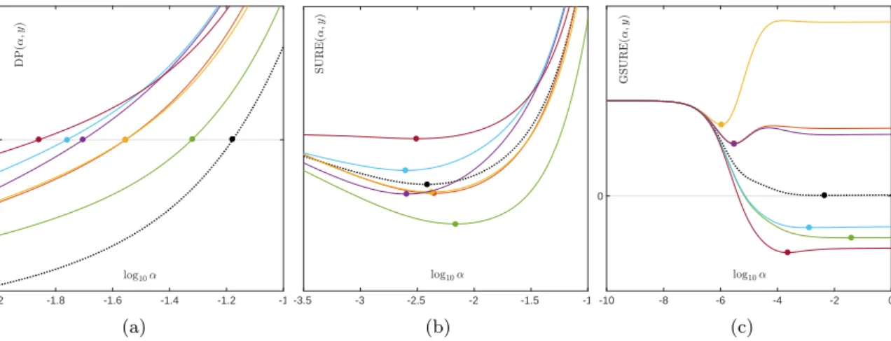
-2 -1.8 -1.6 -1.4 -1.2 -1 log10, 0 D P ( , ;y ) (a) -3.5 -3 -2.5 -2 -1.5 -1 log10, S U R E ( , ;y ) (b) -10 -8 -6 -4 -2 0 0 (c)
Figure 5: True risk functions (black dotted line), their estimates for six different realizations
yk,k = 1. . .6 (solid lines), and their corresponding minima/roots (dots on the lines) in the
setting described in Figure 1 using `2-regularization: (a) DP(α, Ax∗) and DP(α, yk). (b)
RSURE(α) and SURE(α, yk). (c)RGSURE(α) and GSURE(α, yk).
3
Properties of the Parameter Choice Rules for Quadratic
Regularization
In this section we consider the theoretical (risk) properties of SURE, GSURE and the dis-crepancy principle.
Assumption 1. For the sake of simplicity we only consider m = n in this first analysis. Furthermore, we assume
1 =γ1 ≥. . .≥γm>0 (14)
and thatkx∗k2
2 =O(m). Note that all assumptions are fulfilled in the numerical example we
described in the previous section.
We mention that we consider here a rather moderate size of the noise, which remains bounded
in variances as m → ∞. A scaling corresponding to white noise in the infinite dimensional
limit is ratherσ2∼mand an inspection of the estimates below shows that the risk estimate
is potentially far from the expected values in such cases additionally.
3.1 SURE-Risk
We start with an investigation of the well-known SURE risk estimate. Based on (11) and
Stein’s result, the representation for the risk is given as
RSURE(α) =E[SURE(α, y)] =X i α2 (γ2 i +α)2 E[y2i]−σ2m+ 2σ2 X i γi2 γ2 i +α =X i α2 (γ2 i +α)2 (γi2·(x∗i)2+σ2)−σ2m+ 2σ2X i γ2 i γ2 i +α . (15)
Figure5(b)illustrates the typical shape of RSURE(α) and SURE estimates thereof. Following
[35, 14], who investigated the performance of Stein’s unbiased risk estimate in the different
context of hierarchical modeling, we show that, with the definition of the lossl by
l(α) := 1
mkAx
∗−Axˆ
α(y)k22,
1/mSURE(α, y) is close to l for large m. Note that SURE is an unbiased estimate of the
expectation ofl.
Theorem 1. If Assumption 1 holds, then sup α∈[0,∞) 1 mSURE(α, y)−l(α) =OP 1 √ m . Proof: We find l= 1 mkAxˆ−y+εk 2 2 = 1 mkAxˆ−yk 2 2+ 1 mkεk 2 2+ 2 mhε, Axˆ−yi = 1 m m X i=1 α2 (γ2 i +α)2 yi2− 1 mkU ∗εk2 2+ 2 mhε, Axˆ−Ax ∗i = 1 m m X i=1 α2 (γi2+α)2y 2 i − 1 mkε˜k 2 2+ 2 mhε, Axˆ−Ax ∗i. Note that Axˆ−Ax∗ =UΣΣ−α1U∗(Ax∗+ε)−UΣV∗x∗ =U{ΣΣ−α1−I}ΣV∗x∗+UΣΣ−α1U∗ε
and recall from (8) that x∗i =hvi, x∗i.Since U∗U =U U∗ =I, Var[˜εi] =σ2, where ˜ε=U∗ε,
that is, ˜εi=hui, εi. This yields
2 mhε , Axˆ−Ax ∗i = 2 m n X i=1 ˜ ε2iγi2 γ2 i +α − 2 m n X i=1 αε˜iγix∗i γ2 i +α .
We obtain the representation 1 mSURE(α, y)−l=−σ 2+2σ2 m m X i=1 γ2 i γ2 i +α + 1 m m X i=1 ˜ ε2i − 2 m m X i=1 ˜ ε2 iγi2 γ2 i +α + 2 m m X i=1 αε˜iγix∗i γ2 i +α = 1 m m X i=1 (˜ε2i −σ2)− 2 m m X i=1 γ2i γi2+α(˜ε 2 i −σ2) + 2 m m X i=1 αγi α+γi2x ∗ iε˜i =:Sl1(α) +Sl2(α) +Sl3(α),
where the termsSlj(α), j ∈ {1,2,3} are defined in an obvious manner. Since ˜ε21, . . . ,ε˜2n are
independent and identically distributed with expectationσ2 we immediately obtain that
√
mSl1(α) =OP(σ
Note thatSl1(α) is independent of α. Next, we consider the termSl2(α).
Due to the ordering of the singular values the vectorsγi2/(γi2+α), which have entries in (0,1]
forα∈[0,∞), and are monotonically decreasing. Thus, we find
sup α∈[0,∞) |Sl2(α)|= sup α∈[0,∞) 1 m m X i=1 γ2i γ2 i +α (˜ε2i −σ2) ≤ sup 1≥c1≥...≥cm≥0 1 m m X i=1 ci(˜ε2i −σ2) .
It follows from [21], Lemma 7.2.:
sup 1≥c1≥...≥cm≥0 1 m m X i=1 ci(˜ε2i −σ2) = sup 1≤j≤m 1 m j X i=1 (˜ε2i −σ2) ,
and an application of Kolmogorov’s maximal inequality yields: sup
α∈[0,∞)
|Sl2(α)|=OP σ
2/√m ,
where we also used that Var(˜ε2i −σ2) = 2σ4,which follows because ˜εi ∼ N(0, σ2).
Finally, we estimate Sl3(α). The functions α 7→ αγi/(γi2 +α) are monotonically
increas-ing, which implies that αγi/(γi2 +α) ⊂ [0,1], by condition (14). A further application of
Kolmogorov’s maximal inequality finally yields sup α∈[0,∞) |Sl3(α)|= sup α∈[0,∞) 1 m m X i=1 αγi γi2+αx ∗ iε˜i ≤ sup 1≥c1≥...≥cm≥0 1 m m X i=1 cix∗iε˜i = sup 1≤j≤m 1 m j X i=1 x∗iε˜i =OPσkx∗k2/m=OPσ/√m.
The latter result can be used to show that, in an asymptotic sense, if the lossl is considered,
the estimator ˆαSURE does not have a larger risk than any other choice of regularization
parameter. This statement is made precise in the following corollary.
Corollary 1. Under Assumption 1 it holds that for all ε > 0 and any sequence of positive
real numbers (αm)m∈N we have
P(l( ˆαSURE)≥l(αm) +ε)→0.
Proof: By definition SURE( ˆαSURE, y)≤SURE(αm, y). This yields
P(l( ˆαSURE)≥l(αm) +ε)≤P l( ˆαSURE)− 1 mSURE( ˆαSURE, y)≥l(αm)− 1 mSURE(αm, y) +ε
and the claim follows by an application of Theorem1.
The following corollary is an extension of Corollary1.
Corollary 2. The claim of Corollary1remains true if the arbitrary but fixed positive constant
ε >0 is replaced by a sequence εm such that 1/εm=o(
√
We finally mention that our estimates are rather conservative, in particular with respect to
the quantitySl3(α), since we do not assume particular smoothness ofx∗. With an additional
source condition, i.e., certain decay speed of the x∗i, it is possible to derive improved rates,
which are however beyond the scope of our paper. We instead turn our attention to the
convergence of the risk estimate as m → ∞ as well as the convergence of the estimated
regularization parameters.
Theorem 2. If Assumption 1 holds, then, as m→ ∞
sup α∈[0,∞) 1 m SURE(α, y)−RSURE(α, y) =OP 1 √ m and E sup α∈[0,∞) 1 m SURE(α, y)−RSURE(α, y) 2 =O1 m . (16)
Proof: Observing (11) and (15) we find
1 m SURE(α, y)−RSURE(α) = 1 m m X i=1 α2 (γ2 i +α)2 ˇ εi,
where ˇεi:=yi2−E[y2i]. The random variables ˇε1, . . . ,εˇnare independent and centered. Notice
that Var[ˇεi] = Var[y2i] =E[yi4]−(E[yi2])2 = 4γ2ix ∗ i 2 σ2+ 2σ4,
sinceyi ∼ N(γix∗i, σ2). Consider the monotonically increasing function α7→ α
2
(γ2
i+α)2
⊂[0,1]
forα∈[0,∞). With the same arguments as in the proof of Theorem 1, using Kolmogorov’s
maximal inequality, we estimate
sup α∈[0,∞) SURE(α, y)−RSURE(α) = sup α∈[0,∞) m X i=1 α2 (γ2i +α)2εˇi = sup 1≤j≤m j X i=1 ˇ εi =OP m X j=1 (4γ2i(x∗i)2+ 2σ4) 12
It remains to show theL2-convergence (16). To this end define thej-th partial sum
Sj := j X i=1 ˇ εi
and observe that{Sj|j∈N}forms a martingale. TheLp-maximal inequality for martingales
yields E sup α∈[0,∞) 1 m SURE(α, y)−RSURE(α) 2 =E sup α∈[0,∞) 1 m SURE(α, y)−RSURE(α) 2 = 1 m2E sup 1≤j≤m |Sj|2 ≤ 4 m2E m X i=1 ˇ εi 2 =O 1 m2 m X j=1 (4γi2(x∗i)2+ 2σ4)
as above.
In order to understand the behavior of the estimated regularization parameters we start with
some bounds on ˆαSURE∗ , which recover a standard property of deterministic regularization
methods, namely that σα2 does not diverge for suitable parameter choices.
Lemma 1. A regularization parameter αˆ∗SURE obtained from RSURE satisfies
σ2 maxi|x∗i|2 ≤αˆ∗SURE≤max{1,8σ2 P γi4 P γi4(x∗i)2}
Proof: It is straightforward to see the differentiability of RSUREand to compute
RSURE0(α) = m X i=1 2γ4 i (γi2+α)3(α(x ∗ i)2−σ2).
Hence, forα < maxσ2
i|x∗i|2, the risk RSUREis strictly decreasing, which implies the first
inequal-ity. Moreover, forα≥1 we obtain
α3RSURE0(α) = 2 m X i=1 γ4 i (γi2/α+ 1)3(α(x ∗ i)2−σ2) > α 4 m X i=1 γi4(x∗i)2−2σ2 m X i=1 γi4
and we finally see that RSURE0 is nonnegative if in additionα≥8σ2
P γ4 i P γ4 i(x ∗ i)2 .
In order to make the convergence as m → ∞ more clear we make the dependence on m
explicit in the following by writing RSURE,m and α∗SURE,m for the associated estimate of the
regularization parameter. From a straight-forward estimate of the derivative of RSURE,m on
sets where α is bounded away from zero we obtain the following result:
Lemma 2. The sequence of functionsfm := m1 RSURE,m(α)is equicontinuous on sets[C1, C2]
with0< C1< C2.
As a consequence of the Arzela-Ascoli theorem we further derive a convergence result: Proposition 1. The sequence of functions fm := m1 RSURE,m(α) is equicontinuous on sets
[C1, C2] with 0 < C1 < C2 and hence has a uniformly convergent subsequence fmk with
continuous limit function f.
In order to obtain convergence of minimizers it suffices to be able to choose uniform constants
C1 and C2, which is possible if the bounds in Lemma 1are uniform:
Theorem 3. Let maxmi=1|xi∗| be uniformly bounded in m and m1 Pm
i=1γi4(x∗i)2 be uniformly
bounded away from zero. Then there exists a subsequence αˆSURE,mk that converges to a
min-imizer of the asymptotic risk f. Moreover αˆSURE, mk converges to to a minimizer of the
asymptotic riskf in probability.
Proof: From the uniform convergence of the sequence fmk in Proposition 1 we obtain the
convergence of the minimizers ˆα∗SURE,mk. Combined with Theorem 2 we obtain an analogous
argument for ˆαSURE,mk.
3.2 Discrepancy Principle
We now turn our attention to the discrepancy principle, which we can formulate in a similar setting as the SURE approach above. With a slight abuse of notation, in analogy to the other
methods, we denote the expectation of DP(α, y) by RDP(α) and define ˆαDP as the solution
of the equation RDP(α) = m X i=1 α2 (γi2+α)2E[y 2 i]−mσ2 = 0.
Figure5(a) illustrates the typical shape of RDP(α) and its DP estimates. Observing that
DP(α, y)−RDP(α) = SURE(α, y)−RSURE(β)
we immediately obtain the following result: Theorem 4. If Assumption 1 holds, we have
sup α∈[0,∞) 1 m DP(α, y)−RDP(α) =OP 1 √ m and E sup α∈[0,∞) 1 m DP(α, y)−RDP(α) 2 =O 1 m . 3.3 GSURE-Risk
Now we consider the GSURE-risk estimation procedure. Figure 5(c) illustrates the typical
shape of RGSURE(α) and GSURE estimates thereof. Based on (12), the risk can be written
as RGSURE(α, y) = m X i=1 1 γi − γi (γi2+α) 2 γ2i(x∗i)2+σ2−σ2 m X i=1 1 γi2 + 2σ 2 m X i=1 1 γi2+α.
For the SURE criterion we showed in Theorem 1 that SURE(α, y) is close to the loss l in
an asymptotic sense with the standard√m-rate of convergence. An analogous result can be
shown for GSURE and the associated loss ˜l:=cmkΠ(x∗−xˆα)k22 but with different associated
rates of convergencecm, dependent on the singular values.
Theorem 5. Let Assumption 1 be satisfied and in addition to (14), let γm → 0. Then, as
m→ ∞, sup α∈[0,∞) GSURE(α, y)−c −1 m˜l =OP v u u t m X i=1 x∗i γ2 i + v u u t m X i=1 1 γ4 i , where cm:= m X j=1 1 γi2 −1/2 .
Proof: For m=nand invertible matrices A the GSURE-loss ˜lis given by c−m1˜l=kx∗−xˆαk22 = m X i=1 1 γi − γi (γi2+α) 2 yi2− m X j=1 ˜ ε2i γi2 + 2α m X j=1 x∗iε˜ γi(γ2i +α) + 2−2 m X j=1 ˜ ε2i γi2+α,
since, in this special case, the projectionπ satisfiesπ = id.Hence
GSURE(α, y)−c−m1˜l=− m X i=1 1 γi2(˜ε 2 i −σ2) + 2 m X i=1 1 γi2(˜ε 2 i −σ2)−2 m X i=1 1 γ2i +α(˜ε 2 i −σ2) + 2α m X i=1 x∗i γi(γi2+α) ˜ εi = 2α m X i=1 x∗i γi(γi2+α) ˜ εi+ m X i=1 α2−γi4 γi2(γ12+α)2(˜ε 2 i −σ2) =:GSl1(α) +GSl2(α),
whereGSl1(m, α) and GSl2(m, α) are defined in an obvious manner. Furthermore,
sup α∈[0,∞) |GSl1(α)|= sup α∈[0,∞) 2α m X i=1 x∗i γi(γi2+α) ˜ εi = sup 1≥c1≥...≥cm≥0 2 m X i=1 ci x∗i γi ˜ εi = sup 1≤j≤m 2 j X i=1 x∗i γi ˜ εi =OP v u u t m X i=1 x∗i γi2 ,
where the last estimate follows from Kolmogorov’s maximal inequality. Now we estimate the
term GSl2(α). Consider the functions ψi : α 7→ (α2−γi4)/(γi2 +α)2, i = 1, . . . , m. Notice
that
ψi(0) =−1 and lim
α→∞ψi(α) = 1 fori= 1, . . . , m
and that for eachithe functionψi increases monotonically in α. This implies
sup α∈[0,∞) |GSl2(α)|= sup α∈[0,∞) m X i=1 α2−γi4 γi2(γ12+α)2(˜ε 2 i −σ2) ≤ sup 1≥c1≥...≥cm≥0 m X i=1 ci γ2 i (˜ε2i −σ2) + sup 0≤c1≤...≤cm≤1 m X i=1 ci γ2 i (˜ε2i −σ2) ≤ sup 1≤j≤m j X i=1 1 γi2(˜ε 2 i −σ2) + sup 1≤j≤m m X i=j 1 γi2(˜ε 2 i −σ2) .
A further application of Kolmogorov’s maximal inequality yields the desired result.
We can now proceed to an estimate between GSURE and RGSURE similar to the ones for
the SURE risk, however we observe a main difference due to the appearance of the condition
Theorem 6. Let A∈Rn×m be a full rank matrix. In addition to Assumption 1, letγ m →0. Then, asm→ ∞, sup α∈[0,∞) 1
m cond(A)2 GSURE(α, y)−RGSURE(α)
=OP 1 √ m and E sup α∈[0,∞) 1
mcond(A)2 GSURE(α, y)−RGSURE(α)
2 =OP1 m . (17)
Proof: For full rank matrices A∈Rm×m we have
GSURE(α, y) = m X i=1 1 γi − γi (γ2 i +α) 2 yi2−σ2 m X i=1 1 γ2 i + 2σ2 m X i=1 1 γ2 i +α . This gives GSURE(α, y)−RGSURE(α) = m X i=1 1 γi − γi (γ2i +α) 2 y2i −E[y2i] = m X i=1 1 γi − γi (γ2i +α) 2 ˇ εi.
As in the proof of Theorem2we set ˇεi :=y2i −E[y2i].Recall that the random variables ˇεi are
centered, independent with Var[ˇεi] = 4γi2x∗i
2σ2+ 2σ4. We find GSURE(α, y)−RGSURE(α) = 1 γ2 m m X i=1 γm2 γ2 i α2 (γ2 i +α)2 ˇ εi.
With the same arguments as in the proofs of Theorems1 and 2 we obtain
sup α∈[0,∞) GSURE(α, y)−RGSURE(α) ≤ sup 0≤c1≤c2≤...≤1 1 γ2 m m X i=1 ciεˇi ≤1max≤j≤m 1 γ2 m m X i=j ˇ εi .
Again, an application of Kolmogorov’s maximal inequality yields sup α∈[0,∞) GSURE(α, y)−RGSURE(α) =OP 4 m X i=1 γi2x∗i2σ2+ 2mσ4 12!
and the first claim of the theorem follows with cond(A) = γ1/γm = 1/γm. Moreover, in a
similar manner as in the proofs of the previous theorems, we find
E sup α∈[0,∞) 1
m cond(A)2 GSURE(α, y)−RGSURE(α)
2 ≤E sup 1≤j≤m 1 γ2 m Sj 2
and by theLp maximal inequality the second claim now follows as
E sup 1≤j≤m 1 γ2 m Sj 2 ≤ 1 γ4 m ESm2 =O m/γm4 . We finally note that in the best case the convergence of GSURE is slower than that of
SURE. However, since for ill-posed problems the condition number ofAwill grow withmthe
typical case is rather divergence of cond(√A)2
m , hence the empirical estimates of the regularization
parameters might have a large variation, which will be confirmed by the numerical results below.
4 5 6 7 8 9 10 11 log2m -24 -22 -20 -18 -16 -14 -12 -10 -8 -6 lo g2 f ( m ) l= 0:01 l= 0:02 l= 0:03 l= 0:04 l= 0:06 l= 0:08 l= 0:10 c1=m2 c2=m (a) SURE 4 5 6 7 8 9 10 11 log2m 0 50 100 150 200 lo g2 f ( m ) l= 0:01 l= 0:02 l= 0:03 l= 0:04 l= 0:06 l= 0:08 l= 0:10
(b) GSURE, without cond(A)
4 5 6 7 8 9 10 11 log2m -35 -30 -25 -20 -15 -10 -5 lo g2 f ( m ) l= 0:01 l= 0:02 l= 0:03 l= 0:04 l= 0:06 l= 0:08 l= 0:10 c1=m c2=m2
(c) GSURE, with cond(A)
Figure 6: Illustration of Theorems2and6for`2-regularization: The left hand side of (16)/(17)
was estimated by the sample mean and plotted vs. m. For (17), the normalization with
cond(A) was omitted in (b) and included in (c). The black dotted lines were added to
compare the order of convergence.
4
Numerical Studies for Quadratic Regularization
4.1 Setup
As in the illustrative example in Section2.1, we computed the empirical distributions of the
different parameter choice rules for the same scenario (cf. Section2.2) for each combination
of m = n = 16,32,64,128,256,512,1024,2048, l = 0.01,0.02,0.03,0.04,0.06,0.08,0,1 and
σ = 0.1. For m= 16, . . . ,512, Nε = 106 and for m= 1024,2048, Nε= 105 noise realizations
were sampled. The computation was, again, based on a logarithmical α-grid, i.e., log10α
is increased linearly in between -40 and 40 with a step size of 0.01. In addition to the
distributions of α, the expressions
sup α SURE(α, y)−RSURE(α, y) , and sup α GSURE(α, y)−RGSURE(α, y) (18)
were computed over the α-grid. As in some cases, the supremum is obtained in the limit
α → ∞, and hence, on the boundary of our computational grid, we also evaluated (18) for
α =∞ in these cases.
4.2 Illustration of Theorems
We first illustrate Theorems 2and 6by computing (16) and (17) based on our samples. The
results are plotted in Figure 6 and show that the asymptotic rates hold. For GSURE, the
comparison between Figures 6(b) and 6(c) also shows that the dependence on cond(A) is
crucial.
4.3 Dependence on the Ill-Posedness
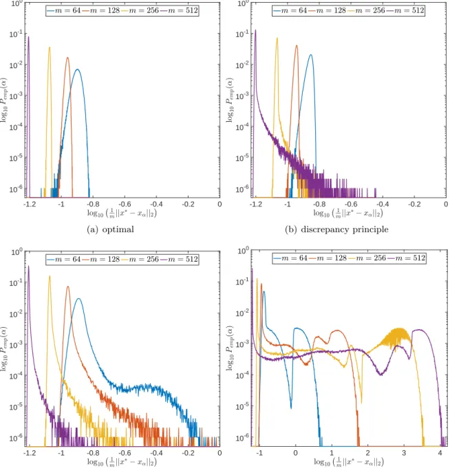
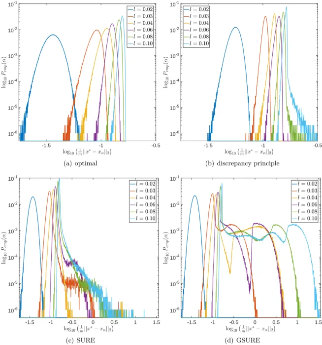
We then demonstrate how the empirical distributions of ˆα and the corresponding `2-error,
kx∗ −xαˆk22, such as those plotted in Figure 3, depend on the ill-posedness of the inverse
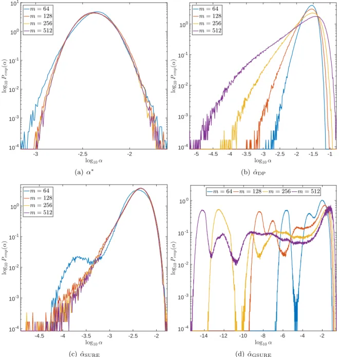
Dependence on m In Figures 7and 8,m is increased while the width of the convolution kernel is kept fix. The impact of this on the singular value spectrum is illustrated in Figure
2. Most notably, smaller singular values are added and the condition of A increases (cf.
Table 1). Figures 7(a) and 8(a) suggest that the distribution of the optimal α∗ is Gaussian
and converges to a limit for increasing m. The distribution of the corresponding `2-error
looks Gaussian as well and seems to concentrate while shifting to larger mean values. For
the discrepancy principle, Figures 7(b) and 8(b) show that the distribution of ˆαDP widens
for increasing m, and the distribution of the corresponding `2-error develops a tail while
shifting to larger mean values. Figures 7(c) and 8(c) show that the distribution of ˆαSURE
seems to converge to a limit for increasingm. The distribution of the corresponding`2-error
also develops a tail while shifting to larger mean values. For GSURE, Figures 7(d)and 8(d)
reveal that increasing m leads to erratic, multimodal distributions: Compared to the other
α-distributions, the distribution of ˆαGSUREincludes a significant amount of very small values,
and the corresponding `2-error distributions range over very large values.
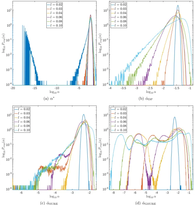
Dependence on l In Figures9 and10, the width of the convolution kernel,l, is increased
while m = 64 is kept fix (cf. Figure 2 and Table 1). It is worth noticing that as l = 0.02
corresponds to a very well-posed problem, the optimal α∗ is often extremely small or even 0,
as can be seen from Figure 9(a). The general tendencies are similar to those observed when
increasing m. For GSURE, Figures9(d) and 10(d) illustrate how the multiple modes of the
distributions slowly evolve and shift to smaller vales ofα(and larger corresponding`2-errors).
4.4 Linear vs Logarithmical Grids
One reason why the properties of GSURE exposed in this work have not been noticed so far
is that they only become apparent in very ill-conditioned problems (cf. Section 1). Another
reason is the way the risk estimators are typically computed: Firstly, for high dimensional
problems, (3) often needs to be solved by an iterative method. For very smallα, the condition
of (A∗A+αI) is very large and the solver will need a lot of iterations to reach a given tolerance.
If, instead, a fixed number of iterations is used, an additional regularization of the solution
to (1) is introduced which alters the risk function. Secondly, again due to the computational
effort, a coarse, linear α-grid excluding α= 0 instead of a fine, logarithmic one is often used
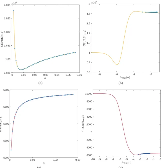
for evaluating the risk estimators. For two of the risk estimations plotted in Figure 5(c),
Figure 11 demonstrates that this insufficient coverage of small α values by the grid can lead
to missing the global minimum and other misinterpretations.
5
Numerical Studies for Non-Quadratic Regularization
In this section, we consider the popular sparsity-inducing R(x) = kxk1 as a regularization
functional (LASSO penalty) to examine whether our results also apply to non-quadratic
regularization functionals. For this, let I be the support of ˆxα(y) andJ its complement. Let
further|I| =k and PI ∈ Rk×n be a projector onto I and AI the restriction of A to I. We
have that
dfα=kxˆα(y)k0=k and gdfα = tr(ΠB[J]), B[J]:=PI(A∗IAI)−1PI∗,
as shown, e.g., in [29,12,10], which allows us to compute SURE (6) and GSURE (7). Notice
allα where the supportI changes.
To carry out similar numerical studies as those presented the last section, we have to overcome several non-trivial difficulties: While there exist various iterative optimization techniques to
solve (2) nowadays (see, e.g., [7]), each method typically only works well for certain ranges
ofα, cond(A) and tolerance levels to which the problem should be solved. In addition, each
method comes with internal parameters that have to be tuned for each problem separately
to obtain fast convergence. As a result, it is difficult to compute a consistent series of ˆxα(y)
for a given logarithmicalα-grid, i.e., that accurately reproduces all the change-points in the
support and has a uniform accuracy over the grid. Our solution to this problem is to use an
all-at-once implementation of ADMM [5] that solves (2) for the whole α-grid simultaneously,
i.e., using exactly the same initialization, number of iterations and step sizes. See Appendix
Afor details. In addition, an extremely small tolerance level (tol= 10−14) and 104 maximal
iterations were used to ensure a high accuracy of the solutions.
Another problem for computing quantities like (18) is that we cannot compute the
expecta-tions defining the real risks RSURE(6) and RGSURE(7) anymore: We have to estimate them as
the sample mean over SURE and GSURE in a first run of the studies, before we can compute
(18) in a second run (wherein RSUREand RGSUREare replaced by the estimates from the first
run).
We considered scenarios with each combination of m = n = 16,32,64,128,256,512, l =
0.02,0.04,0.06 and σ = 0.1. Depending on m, Nε = 105,104,104,104,103,103 noise
realiza-tions were examined. The computation was based on a logarithmicalα-grid where log10α is
increased linearly in between -10 and 10 with a step size of 0.01.
Risk plots Figure 12 shows the different risk functions and estimates thereof. The jagged
form of the SURE and GSURE plots evaluated on this fineα-grid indicates that the underlying
functions are discontinuous. Also note that while SURE and GSURE for each individual noise
realization are discontinuous, RSURE and RGSUREare smooth and continuous, as can be seen
already from the empirical means overNε = 104.
Empirical Distributions Figure 13 shows the empirical distibutions of the different
pa-rameter choice rules forα. Here, the optimal α∗ is chosen as the one minimizing the`1-error
kx∗−xαˆk1to the true solutionx∗. We can observe similar phenomena as for`2-regularization.
In particular, the distributions for GSURE, also have multiple modes at small values ofαand
at large values of`1-error.
Sup-Theorems Due to the lack of explicit formulas for the `1-regularized solution xα(y),
carrying out similar analysis as in Section3 to derive theorems such as Theorems 2and 6 is
very challenging. In this work, we only illustrate that similar results may hold for the case
of `1-regularization by computing the left hand side of (16) and (17) based on our samples.
The results are shown in Figure14 and are remarkably similar to those shown in Figure6.
Linear Grids and Accurate Optimization All the issues raised in Section 4.4 about why the properties of GSURE revealed in this work are likely to be overlooked when working
on high dimensional problems are even more crucial for the case of `1-regularization: For
computational reasons, the risk estimators are often evaluated on a coarse, linear α-grid
illustrates that this may obscure important features of the real GSURE function, such as the
strong discontinuities for smallα, or even change it significantly.
6
Conclusion
From the results presented in this work, we see that unbiased risk estimators encounter enor-mous difficulties for the parameter choice in variational regularization methods for ill-posed problems. While the discrepancy principle yields a quite unimodal distribution of regulariza-tion parameters resembling the optimal one with slightly increased mean value, the SURE estimates start to develop multimodality, and the additional modes consist of underestimated regularization parameters, which may lead to significant errors in the reconstruction.
For the case of GSURE, which is based on a presumably more reliable risk, the estimates produce quite wide distributions (at least in logarithmic scaling) for increasing ill-posedness, in particular there are many highly underestimated parameters, which clearly yield bad recon-structions. We expect that this behavior is rather due to the bad quality of the risk estimators
than the quality of the risk. These findings may be explained by Theorem 6, which indicates
that the estimated GSURE risk might deviate strongly from the true risk function when the
condition number of A is large, i.e. the problem is asymptotically ill-posed as m→ 0.
Con-sequently one might expect a strong variation in the minimizers of GSURE with varyingy
compared to the ones of RGSURE. A potential way to cure those issues is to develop novel
risk estimates for RGSURE that are not based on Stein’s method, possibly it might even be
useful not to insist on the unbiasedness of the estimators.
We finally mention that for problems like sparsity-promoting regularization, the GSURE risk leads to additional issues, since it is based on a Euclidean norm. While the discrepancy principle and the SURE risk only use the norms appearing naturally in the output space of the inverse problem (or in a more general setting the log-likelihood of the noise), the Euclidean norm in the space of the unknown is rather arbitrary. In particular, it may deviate strongly
from the Banach space geometry in `1 or similar spaces in high dimensions. Thus, different
constructions of GSURE risks are to be considered in such a setting, e.g. based on Bregman distances.
A
A Consistent LASSO Solver
We want to solve (2) withR(x) =kxk1 for a large number of different values ofα but need to
ensure that the results are comparable and consistent. For this, we rely on an implementation
of the scaled version of ADMM [5] that carries out the iterations for all α simultaneously,
with the same penalty parameterρfor allαand a stop criterion based on the maximal primal
and dual residuum over allα. Online adaptation of ρ is also performed based on primal and
dual residua for allα. While ensuring the consistency of the results, this leads to sub-optimal
performance for individualα’s which has to be countered by using a large number of iterations
to obtain high accuracies.
Algorithm 1 (All-At-Once ADMM). Given α1, . . . , αNα, ρ >0 (penalty parameter), τ >1,
µ > 1 (adaptation parameters), K ∈ N (max. iterations) and ε > 0 (stopping tolerance),
initialize X0, Z0, U0 ∈ Rn×Nα by 0, and Y = y ⊗1T
Nα, Λ = [α1, . . . , αNα]⊗1n, where 1l
multipli-cation between matrices (Hadamard product).
Fork= 1, . . . , K do:
Xk+1= (A∗A+ρI)−1(A∗Y +ρ(Zk−Uk)) (x−update)
Zk+1= signXk+1+UkmaxXk+1+Uk−Λ/ρ,0 (z−update)
Uk+1=Uk+Xk+1−Zk+1 (u−update) rik+1=X(k·+1,i) −Z(k·+1,i) ∀ i= 1, . . . , Nα (primal residuum) ski+1=−ρ(Z(k·+1,i) −Z(k·,i)) ∀ i= 1, . . . , Nα (dual residuum) (Uk+1, ρ) = (Uk+1/τ, τ ρ) if # n i kr k+1 i k2> µks k+1 i k2 o > Nα/2 (τ Uk+1, ρ/τ) if #ni ks k+1 i k2> µkrki+1k2 o > Nα/2 (Uk+1, ρ) else. (ρ−adaptation) prii =ε √ n+ max(kX(k·+1,i)k2,kZ(k·+1,i)k2)
∀ i= 1, . . . , Nα (primal stop tol)
duali =ε
√
n+ρkU(k·+1,i)k2
∀ i= 1, . . . , Nα (dual stop tol)
stop if krik+1k2< prii ∧ ksik+1k2 < duali ∀ i= 1, . . . , Nα
The algorithm returns both X(k·+1,i) and Z(k·+1,i) as approximations of the solution to (2) with
R(x) =kxk1 and α=αi of which we useZ(k·+1,i) for our purposes as it is exactly sparse due to
the soft-thresholding step (z-update). In the computations, we furthermore initializedρ = 1
and usedτ = 2, µ= 1.1,ε= 10−14 and K= 104.
Acknowledgements. This work of N. Bissantz, H. Dette and K. Proksch has been supported by the Collaborative Research Center “Statistical modeling of nonlinear dynamic processes” (SFB 823, Project A1, C1, C4) of the German Research Foundation (DFG).
References
[1] M. S. C. Almeida and M. a T. Figueiredo,Parameter estimation for blind and non-blind
deblurring using residual whiteness measures., IEEE Transactions on Image Processing
22(2013), no. 7, 2751–63. 2
[2] F. Bauer and T. Hohage, A Lepskij-type stopping rule for regularized Newton methods,
Inverse Problems 21(2005), no. 6, 1975–1991. 2
[3] Gilles Blanchard and Peter Math´e,Discrepancy principle for statistical inverse problems
with application to conjugate gradient iteration, Inverse problems 28 (2012), no. 11,
115011. 2
[4] Peter Blomgren and Tony F Chan,Modular solvers for image restoration problems using
the discrepancy principle, Numerical linear algebra with applications 9 (2002), no. 5,
[5] S. Boyd, N. Parikh, E. Chu, B. Peleato, and J. Eckstein, Distributed optimization and
statistical learning via the alternating direction method of multipliers, Foundations and
Trends in Machine Learning 3(2011), no. 1, 1–122. 20,21
[6] Bj¨orn Bringmann, Daniel Cremers, Felix Krahmer, and Michael M¨oller,The homotopy
method revisited: Computing solution paths of ` 1-regularized problems, arXiv preprint
arXiv:1605.00071 (2016). 19
[7] M. Burger, A. Sawatzky, and G. Steidl, First Order Algorithms in Variational Image
Processing, arXiv (2014), no. 1412.4237, 60. 20
[8] E. J. Candes, C. a. Sing-Long, and J. D. Trzasko,Unbiased Risk Estimates for Singular
Value Thresholding and Spectral Estimators, IEEE Transactions on Signal Processing61
(2013), no. 19, 4643–4657. 2
[9] C. Deledalle, S. Vaiter, J. Fadili, and G. Peyr´e, Stein Unbiased GrAdient estimator of
the Risk (SUGAR) for Multiple Parameter Selection, SIAM Journal on Imaging Sciences
7 (2014), no. 4, 2448–2487. 2
[10] C. Deledalle, S. Vaiter, G. Peyr´e, J. Fadili, and C. Dossal,Proximal Splitting Derivatives
for Risk Estimation, Journal of Physics: Conference Series386 (2012), 012003. 2,19
[11] C. Deledalle, S. Vaiter, G. Peyr´e, J. Fadili, and C. Dossal, Unbiased risk estimation
for sparse analysis regularization, 2012 19th IEEE International Conference on Image
Processing, IEEE, September 2012, pp. 3053–3056. 2
[12] C. Dossal, M. Kachour, J. Fadili, G. Peyr´e, and C. Chesneau,The degrees of freedom of
the lasso for general design matrix, Statistica Sinica23(2013), no. 2, 809–828. 2,19
[13] Y. C. Eldar,Generalized SURE for Exponential Families: Applications to Regularization,
IEEE Transactions on Signal Processing 57(2009), no. 2, 471–481. 2
[14] S. K. Ghoreishi and M. R. Meshkani,On SURE estimates in hierarchical models assuming
heteroscedasticity for both levels of a two-level normal hierarchical model, Journal of
Multivariate Analysis132 (2014), 129–137. 11
[15] R. Giryes, M. Elad, and Y.C. Eldar, The projected GSURE for automatic parameter
tuning in iterative shrinkage methods, Applied and Computational Harmonic Analysis
30(2011), no. 3, 407–422. 2
[16] H. Haghshenas Lari and A. Gholami, Curvelet-TV regularized Bregman iteration for
seismic random noise attenuation, Journal of Applied Geophysics 109 (2014), 233–241.
2
[17] P. C. Hansen, Analysis of Discrete Ill-Posed Problems by Means of the L-Curve, SIAM
Review34 (1992), no. 4, pp. 561–580. 2
[18] P. C. Hansen and D. P. OLeary,The Use of the L-Curve in the Regularization of Discrete
Ill-Posed Problems, SIAM Journal on Scientific Computing14(1993), no. 6, 1487–1503.
[19] Bangti Jin, Jun Zou, et al., Iterative parameter choice by discrepancy principle, IMA
Journal of Numerical Analysis (2012), drr051. 3
[20] O. V. Lepskii, On a Problem of Adaptive Estimation in Gaussian White Noise, Theory
of Probability & Its Applications 35(1991), no. 3, 454–466 (en). 2
[21] K.-C. Li, From Stein’s Unbiased Risk Estimates to the Method of Generalized Cross
Validation, The Annals of Statistics 13(1985), no. 4, The Annals of Statistics. 12
[22] F. Luisier, T. Blu, and M. Unser, Image denoising in mixed Poisson-Gaussian noise.,
IEEE Transactions on Image Processing 20(2011), no. 3, 696–708. 2
[23] J.-C. Pesquet, A. Benazza-Benyahia, and C. Chaux, A SURE Approach for Digital
Sig-nal/Image Deconvolution Problems, IEEE Transactions on Signal Processing 57(2009),
no. 12, 4616–4632. 2
[24] Peng Qu, Chunsheng Wang, and Gary X Shen,Discrepancy-based adaptive regularization
for grappa reconstruction, Journal of Magnetic Resonance Imaging24(2006), no. 1, 248–
255. 3
[25] S. Ramani, T. Blu, and M. Unser, Monte-Carlo sure: a black-box optimization of
reg-ularization parameters for general denoising algorithms., IEEE Transactions on Image
Processing 17 (2008), no. 9, 1540–54. 2
[26] S. Ramani, Z. Liu, J. Rosen, J.-F. Nielsen, and J. A. Fessler, Regularization parameter
selection for nonlinear iterative image restoration and MRI reconstruction using GCV
and SURE-based methods., IEEE Transactions on Image Processing 21 (2012), no. 8,
3659–72. 2
[27] C. M. Stein,Estimation of the Mean of a Multivariate Normal Distribution, The Annals
of Statistics 9 (1981), no. 6, pp. 1135–1151. 2
[28] Gennadii M Vainikko, The discrepancy principle for a class of regularization methods,
USSR computational mathematics and mathematical physics 22(1982), no. 3, 1–19. 2
[29] S. Vaiter, C. Deledalle, and G Peyr´e,The Degrees of Freedom of Partly Smooth
Regular-izers, arXiv (2014), no. 1404.5557v1. 2,19
[30] S. Vaiter, C. Deledalle, G. Peyr´e, C. Dossal, and J. Fadili,Local behavior of sparse
analy-sis regularization: Applications to risk estimation, Applied and Computational Harmonic
Analysis 35(2013), no. 3, 433–451. 2
[31] D. Van De Ville and M. Kocher,SURE-Based Non-Local Means, IEEE Signal Processing
Letters 16(2009), no. 11, 973–976. 2
[32] D. Van De Ville and M. Kocher, Nonlocal means with dimensionality reduction and
SURE-based parameter selection., IEEE Transactions on Image Processing 20 (2011),
no. 9, 2683–90. 2
[33] Y.-Q. Wang and J.-M. Morel,SURE Guided Gaussian Mixture Image Denoising, SIAM
[34] D. S. Weller, S. Ramani, J.-F. Nielsen, and J. A. Fessler, Monte Carlo SURE-based
parameter selection for parallel magnetic resonance imaging reconstruction, Magnetic
Resonance in Medicine71(2014), no. 5, 1760–1770. 2
[35] X. Xie, S. C. Kou, and L. D. Brown,SURE Estimates for a Heteroscedastic Hierarchical
Model, Journal of the American Statistical Association 107 (2012), no. 500, 1465–1479.
-3 -2.5 -2 log10, 10-4 10-3 10-2 10-1 100 101 lo g10 Pem p ( , ) m= 64 m= 128 m= 256 m= 512 (a)α∗ -5 -4.5 -4 -3.5 -3 -2.5 -2 -1.5 -1 log10, 10-4 10-3 10-2 10-1 100 lo g10 Pem p ( , ) m= 64 m= 128 m= 256 m= 512 (b) ˆαDP -4.5 -4 -3.5 -3 -2.5 -2 log10, 10-4 10-3 10-2 10-1 100 lo g10 Pem p ( , ) m= 64 m= 128 m= 256 m= 512 (c) ˆαSURE -14 -12 -10 -8 -6 -4 -2 log10, 10-4 10-3 10-2 10-1 100 lo g10 Pem p ( , ) m= 64 m= 128 m= 256 m= 512 (d) ˆαGSURE
Figure 7: Empirical probabilities of α for `2-regularization and different parameter choice
-1.2 -1 -0.8 -0.6 -0.4 -0.2 0 log10 !1 mjjx$!x,jj2" 10-6 10-5 10-4 10-3 10-2 10-1 100 lo g10 Pem p ( , ) m= 64 m= 128 m= 256 m= 512 (a) optimal -1.2 -1 -0.8 -0.6 -0.4 -0.2 0 log10 !1 mjjx$!x,jj2" 10-6 10-5 10-4 10-3 10-2 10-1 100 lo g10 Pem p ( , ) m= 64 m= 128 m= 256 m= 512 (b) discrepancy principle -1.2 -1 -0.8 -0.6 -0.4 -0.2 0 log10 !1 mjjx$!x,jj2" 10-6 10-5 10-4 10-3 10-2 10-1 100 lo g10 Pem p ( , ) m= 64 m= 128 m= 256 m= 512 (c) SURE -1 0 1 2 3 4 log10 !1 mjjx$!x,jj2" 10-6 10-5 10-4 10-3 10-2 10-1 100 lo g10 Pem p ( , ) m= 64 m= 128 m= 256 m= 512 (d) GSURE
Figure 8: Empirical probabilities of log10 m1kx∗−xαk22
for `2-regularization and different
-20 -15 -10 -5 log10, 10-4 10-3 10-2 10-1 100 101 lo g10 Pem p ( , ) l= 0:02 l= 0:03 l= 0:04 l= 0:06 l= 0:08 l= 0:10 (a)α∗ -4 -3.5 -3 -2.5 -2 -1.5 -1 log10, 10-4 10-3 10-2 10-1 100 101 lo g10 Pem p ( , ) l= 0:02 l= 0:03 l= 0:04 l= 0:06 l= 0:08 l= 0:10 (b) ˆαDP -6 -5 -4 -3 -2 log10, 10-4 10-3 10-2 10-1 100 101 lo g10 Pem p ( , ) l= 0:02 l= 0:03 l= 0:04 l= 0:06 l= 0:08 l= 0:10 (c) ˆαSURE -8 -7 -6 -5 -4 -3 -2 -1 log10, 10-4 10-3 10-2 10-1 100 101 lo g10 Pem p ( , ) l= 0:02 l= 0:03 l= 0:04 l= 0:06 l= 0:08 l= 0:10 (d) ˆαGSURE
Figure 9: Empirical probabilities of α for `2-regularization and different parameter choice
-1.5 -1 -0.5 log10!m1jjx$!x,jj2" 10-6 10-5 10-4 10-3 10-2 10-1 lo g10 Pem p ( , ) l= 0:02 l= 0:03 l= 0:04 l= 0:06 l= 0:08 l= 0:10 (a) optimal -1.5 -1 -0.5 log10!m1jjx$!x,jj2" 10-6 10-5 10-4 10-3 10-2 10-1 lo g10 Pem p ( , ) l= 0:02 l= 0:03 l= 0:04 l= 0:06 l= 0:08 l= 0:10 (b) discrepancy principle -1.5 -1 -0.5 0 0.5 1 1.5 log10 !1 mjjx$!x,jj2" 10-6 10-5 10-4 10-3 10-2 10-1 lo g10 Pem p ( , ) l= 0:02 l= 0:03 l= 0:04 l= 0:06 l= 0:08 l= 0:10 (c) SURE -1.5 -1 -0.5 0 0.5 1 1.5 log10 !1 mjjx$!x,jj2" 10-6 10-5 10-4 10-3 10-2 10-1 lo g10 Pem p ( , ) l= 0:02 l= 0:03 l= 0:04 l= 0:06 l= 0:08 l= 0:10 (d) GSURE
Figure 10: Empirical probabilities of log10 m1kx∗−xαk22
for`2-regularization and different
0 0.01 0.02 0.03 0.04 0.05 0.06 , 1.829 1.83 1.831 1.832 1.833 1.834 G S U R E ( , ;y ) #104 (a) -8 -6 -4 -2 log10(,) 0.6 0.8 1 1.2 1.4 1.6 1.8 2 G S U R E ( , ;y ) #104 (b) 0 0.01 0.02 0.03 , -5900 -5800 -5700 -5600 -5500 G S U R E ( , ;y ) (c) -10 -9 -8 -7 -6 -5 -4 -3 -2 -1 0 log10(,) -6000 -4000 -2000 0 2000 4000 6000 8000 10000 G S U R E ( , ;y ) (d)
Figure 11: Illustration of the difference between evaluating the GSURE risk on a coarse,
linear grid for α as opposed to a fine, logarithmic one: In (a), a linear grid is constructed
around ˆαDP asα= ∆α,2∆α, . . . ,50∆α with ∆α= 2 ˆαDP/50. While the plot suggests a clear
minimum,(b)reveals that it is only a sub-optimal local minimum and that the linear grid did
not cover the essential parts of GSURE(α, y). (c) and(d)show the same plots for a different
noise realization. Here, a linear grid will not even find a clear minimum. Both risk estimators
-1.5 -1 -0.5 log10, 0 D P ( , ;y ) (a) DP -4 -3.5 -3 -2.5 -2 -1.5 -1 -0.5 log10, 0 S U R E ( , ;y ) (b) SURE -6 -5 -4 -3 -2 -1 0 1 log10, 0 G S U R E ( , ;y ) (c) GSURE
Figure 12: Risk functions (black dotted line), k = 1, . . . ,6 estimates thereof (solid lines)
and their corresponding minima/roots (dots on the lines) in the setting described in Figure
1 using `1-regularization: (a) DP(α, Ax∗) and DP(α, yk). (b) RSURE(α) (empirical mean
over Nε = 104) and SURE(α, yk). (c) RGSURE(α) (empirical mean over Nε = 104) and
GSURE(α, yk). -6 -5 -4 -3 -2 -1 0 log10, 0 0.01 0.02 0.03 Pem p ( , ) ,$ `1 ^ ,DP ^ ,SURE ^ ,GSURE (a) 0 0.5 1 1.5 2 2.5 3 log10jjx$!x,jj1 0 0.02 0.04 0.06 0.08 0.1 Pem p ( , ) ,$ `1 ^ ,DP ^ ,SURE ^ ,GSURE (b)
Figure 13: Empirical probabilities of (a) α and (b) the corresponding `1-error for different
parameter choice rules using `1-regularization, m =n= 64, l = 0.06, σ = 0.1 and N = 104
4 5 6 7 8 9 log2m -18 -16 -14 -12 -10 -8 lo g2 f ( m ) l= 0:02 l= 0:04 l= 0:06 c2=m2 c1=m (a) SURE 4 5 6 7 8 9 log2m -30 -25 -20 -15 -10 lo g2 f ( m ) l= 0:02 l= 0:04 l= 0:06 c1=m c2=m2 (b) GSURE
Figure 14: Illustration that Theorems2 and6 might also hold for `1-regularization: The left
hand side of (16)/(17) is estimated by the sample mean and plotted vs. m. The black dotted
0 0.05 0.1 0.15 0.2 , 66 67 68 69 70 71 72 73 74 G S U R E ( , ;y ) (a) -5 -4 -3 -2 -1 0 1 log10, 0 50 100 150 G S U R E ( , ;y ) (b) 0 0.05 0.1 0.15 , -96 -95 -94 -93 G S U R E ( , ;y ) (c) -6 -4 -2 0 log10, -100 -50 0 50 100 150 G S U R E ( , ;y ) Impl A Impl B (d)
Figure 15: Illustration of the difficulties of evaluating the GSURE risk in the case
of `1-regularization: In (a), a coarse linear grid is constructed around ˆαDP as α =
∆α,2∆α, . . . ,20∆α with ∆α = ˆαDP/10. Similar to Figure 11(a) the plot suggests a clear
minimum. However, using a fine, logarithmic grid,(b)reveals that it is only a sub-optimal
lo-cal minimum before a very erratic part of GSURE(α, y) starts. (c)shows how a coarse α-grid
can lead to an arbitrary projection of GSURE(α, y) that is likely to miss important features.
Both risk estimators are the same as those plotted in Figure12(c) with the same colors. In
(d), the difference between computing GSURE(α, y) with the consistent and highly accurate
version of ADMM (Impl A) and with a standard ADMM version using only 20 iterations (Impl B) is illustrated.