Production planning and control of closed-loop supply chains
Karl InderfurthOtto-von-Guericke University Magdeburg, Faculty of Economics and Management, P.O.Box 4120, 39016 Magdeburg, Germany, [email protected]
Ruud H. Teunter
Erasmus University Rotterdam, Econometric Institute, P.O.Box 1738, 3000 DR Rotterdam, The Netherland, [email protected]
Econometric Institute Report EI 2001 - 39 1. Introduction
Closed-loop supply chains are characterized by the recovery of returned products. In most of these chains (e.g. glass, metal, paper, computers, copiers), used products (also known as cores) are returned by or collected from customers. But returned products can also come from production facilities within the supply chain (production
defectives, by-products. In cases with internal returns, recovery is often referred to as rework.
There are two main types of recovery: remanufacturing (product/part recovery) and recycling (material recovery). Energy recovery via incineration could be considered as a third type. Combinations of different recovery types are also possible. It is often not easy to decide what the best product recovery strategy is. Moreover, for a number of reasons, it is difficult to plan and control operations in closed-loop supply chains.
Based on a literature review, [Guide 2000] lists the following complicating
characteristics for planning and controlling a supply chain with remanufacturing of external returns:
1. The requirement for a reverse logistics network 2. The uncertain timing and quality of cores 3. The disassembly of cores
4. The uncertainly in materials recovered from cores
5. The problems of stochastic routings for materials and highly variable processing times.
6. The complication of material matching restrictions
7. The need to balance returns of cores with demands for remanufactured products.
Many of these complicating issues also characterize the planning and control of a supply chain with remanufacturing of internal returns, though often to a lesser degree. We discuss each of the seven complicating characteristics separately, and also
mention an additional one.
The first three complicating characteristics concern closed-loop supply chains with external returns in general (with remanufacturing, recycling, incineration, or
combinations of these recovery options). Cores have to be collected from end-users before they can be recovered. This requires decisions on the number of collection points (take-back centers), incentives for core returns, and transportation methods
from the collection points to recovery facilities (characteristic 1). The timing of a return depends on the uncertain life of a product, and the quality of a return is
influenced by the uncertain intensity of use. These uncertainties complicate capacity planning and inventory control for recovery operations (characteristic 2). A core can often be disassembled in many different ways. This requires decisions on the type of disassembly, e.g. partial or complete, destructive or non-destructive (characteristic 3).
The remaining characteristics only concern remanufacturing systems. Due to the uncertain quality of cores, there is uncertainty about the possibility to remanufacture parts/materials (characteristic 4). The uncertain quality of cores also causes stochastic routings for materials and highly variable processing times (characteristic 5). In some industries (e.g. aviation), it is required that a product/component is remanufactured using the original 'serial-number-specific' parts (characteristic 6). Finally, there is a need to balance core returns and demands for remanufactured products (characteristic 7). Imperfect correlation between demands and returns may lead to excess stocks of repaired/remanufactured products/components. This holds especially if there are different needs for components/parts of the same product, since those
components/parts are normally disassembled at the same time.
We want to mention an additional complicating characteristic for supply chains where products are manufactured as well as remanufactured, i.e., closed-loop supply chains of original equipment manufacturers (OEMs). In such chains, the manufacturing and remanufacturing operations have to be coordinated (characteristic 8) to prevent capacity shortages and excess stocks.
The planning and control of supply chains with internal returns also suffers from many of the above mentioned characteristics (2-5,7,8). Often this is to a lesser degree, due to reduced uncertainties. But on the other hand, returns are immediate and hence jointly planning and controlling production and rework operations can be even more crucial. Moreover, production and rework operations often share the same resources and produced/reworked products compete for the same storage space.
Due to all these complicating characteristics, planning and controlling a closed-loop supply chain is a complex task. Well-known concepts and techniques for
planning/controlling supply chains are not always (directly) useful for closed-loop supply chains. Researchers have therefore developed new techniques or proposed modifications of existing techniques. In this chapter, we will discuss some of their findings. We remark that only the, in our view, most practical findings will be discussed. We refer interested readers to [Gungor and Gupta 1999] for a recent and complete overview of all the findings in this research area.
The remainder of the chapter is organized as follows. In Section 2 we restrict our focus on disassembly and recovery operations in closed-loop supply chains. We discuss methods for finding all possible disassembly/recovery strategies, for comparing those strategies, for picking the best one, and for scheduling the
disassembly/recovery operations. In Sections 3 and 4 we consider the whole closed-loop supply chain, with respectively external and internal returns. In those sections, we discuss methods for jointly planning and controlling disassembly, recovery, assembly, and (for OEMs) manufacturing operations. We end with some concluding remarks in Section 5.
2. Disassembly and recovery
Disassembly may be defined as a systematic method for separating a product into its constituent modules, parts, etc. (all to be called assemblies from now on) [Gupta and Veerakamolmal 1994]. Disassembly plays an important role in product recovery [Jovane et al. 1993]. Obviously, assemblies have to be disassembled before they can be recovered. But even products that are recovered as a whole, e.g. copier machines that are sold on a secondary market, often require partial or complete disassembly, followed by cleaning, testing, and possible repair/replacement of assemblies, before they can be reassembled. Exceptions are products that can be re-used directly, e.g. containers and unopened commercial returns. Many companies, e.g. Air France, Lufthansa, BMW, Volkswagen, Daimler-Chrysler, Nissan, Océ, Xerox and Philips, operate large-scale disassembly plants.
In many cases disassembly is not simply the reverse of assembly. The operational aspects of disassembly are quite different from those of assembly systems [Brennan et al. 1994, Lambert 1999]. Some of the key aspects of disassembly systems are the following:
• There is uncertainty about the timing and number of core returns.
• There is uncertainty about the quality of cores (and their assemblies).
• Cores may not need to be disassembled completely.
• One can choose between disassembly processes (destructive, non-destructive), depending on the type of recovery that is aimed for.
• There is a large number of demand sources (one for each assembly) and a corresponding need for multiple demand forecasts.
Due to these complicating aspects, a disassembly system is difficult to control.
Below, we will present a list of steps that can be used as a guideline for the control of a disassembly system. Afterwards, these steps will be discussed in detail. Ideally, all steps should be considered in the listed order. We remark that product design issues (design for recovery (DFR), design for disassembly (DFD)) are considered to be outside the scope of this chapter, and are therefore not included in the list. We refer interested readers to [Moyer and Gupta 1997] for a review of DFR and DFD in the electronics industries. The list of steps is as follows:
1. (for each type of core) Based on technical and environmental restrictions, identify all possible/efficient disassembly strategies. A disassembly strategy is
characterized by the disassembly set (the set of assemblies that are disassembled), by the disassembly processes, and by the disassembly sequence. Note that there can be multiple disassembly strategies with the same disassembly set, but with different disassembly processes and/or a different disassembly sequence. We remark that the possibilities for disassembling a core can depend on its quality. If so, then each disassembly strategy is actually a collection of disassembly
strategies for every possible state of the core. The quality can be assessed through initial testing of the core and/or testing of assemblies at a later stage.
2. (for each disassembly strategy of each type of core) Identify the recovery options (e.g. remanufacturing, recycling, incineration) for each of the assemblies in the
disassembly set. We remark that the availability of a recovery option for a disassembled assembly can depend on the disassembly processes. For instance, remanufacturing an assembly might be an option after carefully removing it from a core (non-destructive disassembly), but not after tearing it from the core by brute force (destructive disassembly). We further remark that the availability of a
recovery option for an assembly can depend on its quality (see the first step). We will call the combination of a disassembly strategy and of a recovery option for each of the assemblies in the disassembly set, a disassembly/recovery strategy. 3. (for each disassembly/recovery strategy of each type of core) Determine the net
profit of a strategy, by adding the net profits associated with recovery,
disassembly and disposal. That is, add the net recovery revenues for all assemblies in the disassembly set, and subtract all disassembly costs and disposal costs. 4. (for each type of core) Based on a comparison of the net profits of
disassembly/recovery strategies (and possibly also based on environmental legislation and/or on a comparison of the environmental impact of strategies), choose the best disassembly/recovery strategy.
5. (for all types of cores together, given the disassembly/recovery strategy for each type of core that has been chosen in the previous step) Forecast demands for all assemblies that are in the disassembly set of one or more types of cores, and use those forecasts to schedule the disassembly operations (disassembly scheduling). Note that an assembly might be in the disassembly set of multiple types of cores, i.e. there can be 'component commonality'. Furthermore, disassembly operations for different types of cores might share the same equipment. Hence, scheduling the disassembly operations for all types of cores together is a complex task.
To the best of our knowledge, no researchers have addressed all these steps. However, many authors discussed one or more of the steps and proposed/tested methods that can aid in performing those steps. In the remainder of this section, we will discuss and sometimes modify some of their findings. This is done for Steps 1 and 2 in Section 2.1, for Steps 3 and 4 in Section 2.2, and for Step 5 in Section 2.3.
2.1. Steps 1 and 2: Identifying/comparing all possible disassembly strategies and the associated recovery options
In identifying all possible/efficient disassembly strategies for a core, the key role is played by the geometrical structure, though mechanical factors such as force and friction are also relevant [Chen et al. 1997, Dutta and Woo 1995]. The feasibility of recovery options associated with a disassembly strategy depends on technical, commercial, and ecological feasibility criteria [Krikke et al. 1998]. We will not discuss these technical issues in detail here, since our focus is on the optimal control of a disassembly system. We shall simply assume that the set of possible/efficient disassembly strategies and the associated recovery options are given, and focus on comparing the strategies in that set. For ease of presentation, we first assume that there are no variations in the quality of assemblies or uncertainties about disassembly yields. At the end of this section, however, we will discuss situations where these assumptions do not hold.
The easiest way to compare disassembly strategies is by representing them in a disassembly graph/tree, based on the geometrical structure of the product [Arai et al. 1995, Chen et al. 1997, Dutta and Woo 1995, Johnson and Wang 1998, Krikke et al.
1998, Lambert 1997 1999, Penev and de Ron 1996, Pnueli and Zussman 1997, Spengler et al. 1997, Veerakamolmal et al. 1998a, Yan and Gu 1994, Zussman et al. 1994]. Recall from the previous section, that the availability of a recovery option for a certain assembly can depend on the processes that are used to disassemble it. This holds especially for the remanufacturing option, which is only available if an assembly is obtained via non-destructive disassembly. Hence, it seems best to compare strategies in a disassembly graph that indicates the availability of recovery options. Furthermore, this graph should allow multiple disassembly strategies with the same disassembly set, but with different disassembly operations and/or a different disassembly sequence (see also the previous section).
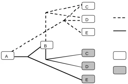
An example of such a disassembly graph for a product is given in Figure 1.
There, we assume that there are two recovery options for assemblies: recycling and remanufacturing. Moreover, all assemblies (including the product A and module B) can be recycled, and remanufacturing is only possible after non-destructive
disassembly. We remark that these assumptions are for clarity of representation only. In Section 2.2, we show how such a disassembly graph can be used to determine the optimal disassembly/recovery strategy.
Figure 1
Variations in the quality of assemblies and uncertainties about disassembly yields can easily be incorporated in a disassembly tree. An assembly with a number of quality classes can be copied into the same number of assemblies. Uncertain disassembly yields can be modeled by splitting disassembly lines. Consider the 3-part product in Figure 1, for instance, and assume that Part E is not always remanufacturable after non-destructive disassembly. Then Figure 1 can be modified accordingly, by splitting the disassembly line from the product A to a remanufacturable Part E into two lines (one to the remanufacturable Part E and the other to the non-remanufacturable Part E) and indicating the associated probabilities. See also [Krikke et al. 1998 1999].
2.2. Steps 3 and 4: Determining the best disassembly/recovery strategy Let us continue the example of Section 2.1 that was graphically represented in Figure 1. Assume that the net profits associated with recovery, disassembly, and disposal are as given in Table 1. Note that the net recycling profits for the product and for the module are smaller than the summed net recycling profits for their parts. This is a result of the increased material-purity when recycling is preceded by disassembly.
Table 1. Net profits for the 3-part product (see Figure 1).
Product A Module B Part C Part D Part E Disposal -4 -3 -1 -2 -1 Recycling 4 3 2 3 2 Remanufacturing -- -- 4 4 10 Destructive disassembly -3 -1 -- -- --Non-destructive disassembly -5 -5 -- --
--Using Figure 1 and Table 1, it is easy to determine the net profit of any disassembly/recovery strategy. Consider, for instance, the following strategy:
disassemble a core in a destructive way, and recycle all three parts. The net profit of this policy is –3+2+3+2=4. By comparing the net profits of all possible
disassembly/recovery strategies, the best strategy can be determined. For this example, the optimal strategy is: disassemble a core in a non-destructive way,
remanufacture Part E, disassemble module B in a destructive way, and recycle Parts C and D. The associated net profit is –5+10-1+2+3=9.
Of course, for products with many modules/parts, the number of possible
disassembly/recovery strategies can be enormous. Fortunately, the disassembly tree-structure can be exploited to determine the best (profit maximizing) strategy in an efficient way using either dynamic programming (DP) [Krikke et al. 1998 1999, Penev and de Ron 1996] or mixed-integer linear programming (MILP) [Johnson and Wang 1998, Lambert 1999, Spengler et al. 1997]. In our view, DP is the easiest and most insightful approach, and hence we will illustrate its use for the product depicted in Figure 1.
The DP algorithm first considers decisions for the lowest level items (Parts C, D and E in Figure 1) and then 'moves up' in the tree until it reaches the root level (the product itself). So we first consider the three parts. Based on the net profits given in Table 1, it is easy to see that (for all parts) recycling is the best available recovery option after destructive disassembly, and that remanufacturing is the best option after non-destructive disassembly. Next consider Module B. The net profits associated with destructive and non-destructive disassembly are respectively –1+2+3=4 and –
5+4+4=3. So Module B should be disassembled in a destructive way, after which Parts C and D should be recycled. Finally consider the product A. The net profits associated with destructive and non-destructive disassembly are respectively – 3+2+3+2=4 and –5+(-1+2+3)+10=9. So the best strategy is as mentioned before.
The DP algorithm can also be used if assemblies vary in quality and if disassembly yields are uncertain. Recall from the previous section, that the disassembly tree should be modified in those cases by introducing multiple quality copies of assemblies and by splitting disassembly lines. To illustrate that DP still works, consider the product in Figure 1 again, but assume that Part E is remanufacturable after non-destructive disassembly in only 80 per cent of the cases (no quality variations or other yield uncertainties). Then the net profits associated with destructive and non-destructive disassembly of the product are respectively –3+2+3+2=4 and
–5+(-1+2+3)+(0.8*10+0.2*2)=7.4. So the best strategy remains unchanged, though the associated net profit is lower.
We end this section with a remark on the net profits for recovery options. We
assumed throughout this section that the profit for recovering an assembly is fixed and hence independent of the number of assemblies that are recovered. As a result, all assemblies of a certain type are recovered in the same (best) way. This seems reasonable for assemblies that are recycled, since demand for the resulting raw materials is (almost) unlimited. But the limited demand/need for remanufactured assemblies might make it unprofitable to remanufacture all the available assemblies. In such cases, different recovery strategies should be used for cores, depending on the demand for remanufactured assemblies in various markets. This issue of limited demand is also relevant for disassembly scheduling, which will be discussed in the next section.
2.3. Step 5: Disassembly scheduling
After completing Steps 1 to 4, the disassembly strategy for each type of core is fixed. What remains is to schedule the disassembly operations for all types of cores. This is a complex task. Compared to assembly scheduling in a traditional assembly
environment, there are two important complicating factors. First, there is a separate demand source for each assembly that is in the disassembly set of one or more types of cores. Second, there is uncertainty about the timing and numbers of core returns.
Researchers [Gupta and Veerakamolmal 1994, Veerakamolmal and Gupta 1998b, Taleb et al. 1997ab] on disassembly scheduling have circumvented these
complications. They focus on a planning horizon for which demands are fixed and known. They further assume that unlimited numbers of cores are available, and that all disassembly lead times are fixed. Under these strict assumptions, the problem of finding the best disassembly schedule is still tractable.
In fact, under the above restrictions, the optimal disassembly schedule can be determined using integer programming (IP) [Veerakamolmal and Gupta 1998b]. However, as is remarked in [Taleb and Gupta 1997b], the computational complexity of IP is considerable for large systems. Alternatively, one can use a heuristic
procedure to find a reasonable, though not necessarily optimal, disassembly schedule. We end this section with a summary of the heuristic approach that is proposed in [Taleb and Gupta 1997b]. This approach is only valid under the previously mentioned assumptions, but it does allow for the existence of common parts and/or materials in different products.
In the first step of the heuristic approach [Taleb and Gupta 1997b], the 'core'
algorithm ignores the timing of the demands for assemblies, and determines a feasible (satisfying all demands over the entire planning horizon) set of cores that have to be disassembled. In building that feasible set of cores, cores are added sequentially based on the associated profit and on the remaining demands for assemblies. After a feasible set has been determined, the 'allocation' algorithm then determines the exact times at which the disassembly of cores in the set should start.
3. Closed-loop supply chains with external returns 3.1. Planning and Scheduling Issues
In Section 2, we discussed methods for comparing product disassembly and recovery strategies. In this section, we will discuss planning and scheduling issues for closed-loop supply chains with external returns if a remanufacturing strategy is chosen. So we consider cases where either whole cores or certain assemblies of cores are
remanufactured. Recall from Section 1 that these are the most complicated cases from a production planning and control (PPC) point of view. Tasks like demand
management, master production scheduling, capacity planning, materials requirements planning and production scheduling have to cope with many complicating characteristics.
Demand management has to tackle the problem of balancing demands for remanufactured products with returns of remanufacturable cores. Since
remanufacturing capabilities are restricted by the inflow of cores, demand planning depends on the degree of knowledge a firm has about the inflow process. Typically, this degree is low. Due to the occurrence of major uncertainties it is very difficult to predict the number of remanufacturable products that will become available in future time intervals. Main sources of uncertainty result from limited predictability of quantity and timing of core returns as well as of core quality and material recovery rates. Suitable forecasting procedures [e.g. Goh and Varaprasad 1986, Krupp 1992] and core sourcing activities [e.g. Krupp 1993] are measures to limit major
uncertainties. Thus it is obvious that in a remanufacturing environment an integrated demand and returns management is necessary.
Material and capacity requirements planning faces uncertain processing operations and uncertain material requirements caused by variations in the quality of used
products. This requires restructuring of both the bill of material (BOM) and the bill of resources (BOR) as well as adjustments in planned lead times. Integrated disassembly and assembly BOMs and specific (quality-dependent) BOMs for different
disassembly and remanufacturing options have been suggested [Krupp 1993, Flapper 1994]. Yield and leadtime adjustments have to protect against major uncertainties in recovery rates and processing times. Material matching faces specific challenges in situations where core suppliers stay owners of the products and require that the same units be returned [Guide and Srivastava 1998].
Uncertainties in routings and material processing times require modified BOR approaches for both rough-cut capacity planning and capacity requirements planning [Dowlatshahi 2000]. [Guide and Spencer 1997a] propose to modify the BOR
calculations using empirical (and regularly updated) occurrence factors for variable routings and material recovery rate factors for probabilistic recovery yields. They show that modified rough-cut capacity planning BOR techniques outperform the standard approaches [Guide et al. 1997].
For all these PPC tasks, it is most of all the high level and variety of uncertainties that require modifications in PPC systems for remanufacturing environments. In this respect, it is important to distinguish between companies that are only engaged in the remanufacturing business and those that also manufacture original products or components, i.e. OEMs.
Uncertainty in the remanufacturing environment may be smaller for OEMs. Better knowledge of original products and their markets, potential application of lease contracts, higher efforts in design for remanufacturing and other factors allow for higher predictability of returns and more standardization and stability in the
remanufacturing processes. Thus planning and scheduling tasks are confronted with less complexity. On the other hand, for materials planning there is the additional problem of coordinating manufacturing and remanufacturing activities (see Section 1). This challenging coordination problem will be treated in more detail in the following section.
3.2. Materials Planning for OEMs
Materials planning in a hybrid manufacturing/remanufacturing environment is concerned with both disassembly and reassembly stages, in order to take the material impact from remanufacturing fully into account. Thus a large number of different options in materials treatment including the option to dispose of parts, components or even cores has to be integrated in the planning system. Even if uncertainties do not play a major role, this complex task cannot be fulfilled by simple MRP-based approaches, but has to be tackled by advanced planning methods. In [Clegg et al. 1995] and [Uzsoy and Venkatachalam 1998] linear programming (LP) models are suggested for optimal decision support in such difficult materials planning situations. In a more practical-oriented approach, the problem is simplified by separating the disassembly part from the combined reassembly and manufacturing part. Disassembly planning is carried out as described in Section 1 leading to standard options, which are chosen mainly depending on the quality of returned products. Thus given or expected return volumes of remanufacturable components or products are available for coordinated materials planning for manufacturing and remanufacturing processes.
Under the separation described above, it will be shown how the standard MRP approach can be extended to incorporate return flows and availability of components or products after disassembly and remanufacturing operations in a hybrid system. We remark that there is widespread use of standard PPC systems, including MRP systems for material procurement [Panisset 1988], in the remanufacturing business. This holds especially for firms employing a make-to-stock strategy [Guide 2000].
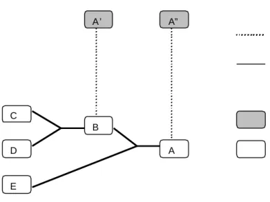
As an example we use the product introduced in Figure 1 and direct our attention to joint disassembly/reassembly and regular manufacturing operations. Figure 2 shows the original manufacturing steps for producing product A as well as additional
opportunities for regaining subassembly B from a low quality core A' or regaining the entire product A from a high quality core A".
Figure 2
Lead times for respective operations are given in Table 2.
Table 2.Lead times for the manufacturing/remanufacturing example.
Operations A from B+E B from C+D A from A" B from A' E D C
As for systems without remanufacturing options, MRP can be applied in a level-by-level procedure performing the standard steps like exploding the BOM, netting gross requirements, lotsizing and offsetting order releases. The coordination problem arises for those components that can be remanufactured as well as manufactured. In order to demonstrate the MRP extensions necessary for coping with the coordination task, we will demonstrate the respective MRP calculations for subassembly B which can either be produced from parts C and D or regained from used core A'.
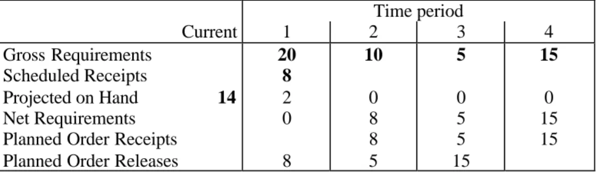
For clarifying the specific extensions, we first present the standard MRP record (without a remanufacturing option) in Table 3. The numbers in bold are input data. Standard MRP calculations lead to the complete MRP record. Safety stocks and lot sizing are not considered in this example.
Table 3. Standard MRP record for subassembly B.
Time period Current 1 2 3 4 Gross Requirements Scheduled Receipts Projected on Hand 14 Net Requirements Planned Order Receipts Planned Order Releases
20 8 2 0 8 10 0 8 8 5 5 0 5 5 15 15 0 15 15
If we include the remanufacturing option, then a number of lines have to be added to the standard MRP record. These provide information on the expected number of remanufacturable core returns, projected on-hand inventory of remanufacturables as well as planned order receipts, planned order releases and scheduled receipts
concerning remanufacturing. If there is a disposal option for remanufacturables, then an additional line with information on planned order releases for disposal has to be included.
Furthermore, a priority rule for fulfilling net requirements is needed. For instance, remanufacturing could always be given priority over manufacturing (as long as
remanufacturables are available). This rule is sensible if remanufacturing is less costly than manufacturing. If there is a disposal option for remanufacturables, then a
disposal decision rule is also needed. For instance, limit to stock of remanufacturables to a certain threshold. That threshold may be the storage capacity or may result from an economic trade-off between holding costs and (remanufacturing versus
manufacturing) cost savings [Inderfurth and Jensen 1999].
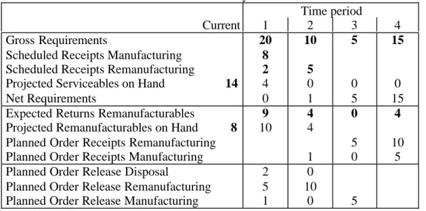
Table 4 gives the extended MRP record. Compared to Table 3, it includes additional input data the expected return flows and on the current stock of remanufacturables. The ‘remanufacturing first’ priority rule is employed, and a disposal limit of 10 items is prespecified. Table 4 shows how planned order releases for all activities (disposal, remanufacturing and manufacturing) develop over time, taking into consideration the respective lead times. As in Table 3, the numbers in bold are input data.
Table 4. Extended MRP record for subassembly B.
Time period
Current 1 2 3 4
Gross Requirements
Scheduled Receipts Manufacturing Scheduled Receipts Remanufacturing
Projected Serviceables on Hand 14
Net Requirements 20 8 2 4 0 10 5 0 1 5 0 5 15 0 15 Expected Returns Remanufacturables
Projected Remanufacturables on Hand 8
Planned Order Receipts Remanufacturing Planned Order Receipts Manufacturing
9 10 4 4 1 0 5 0 4 10 5 Planned Order Release Disposal
Planned Order Release Remanufacturing Planned Order Release Manufacturing
2 5 1 0 10 0 5
We remark that alternative decision rules can also be applied. The push-rule, for instance, suggests to immediately remanufacture all units available. Of course, this will lead to order releases different from those presented in Table 3. In addition to implementing the MRP approach in a rolling horizon framework, uncertainties in returns and leadtimes can be taken into account by using safety stocks and/or safety lead times as means of protection. In this situation not only determining the size of the safety stock but also dividing it between serviceable and remanufacturable items is a relevant issue. Recent research gives some indication that compared to decision rules from stochastic inventory control an appropriate implementation of safety stocks and – under specific conditions – of safety lead times guarantees a high level of MRP performance even in situations with considerable uncertainties [Inderfurth 1998, Gotzel and Inderfurth 2001].
The cost-optimal determination of safety stocks in a hybrid
manufacturing/remanufacturing system is a very challenging problem. Helpful
support for its solution can be given by stochastic inventory control models, which are addressed in another chapter of this book. Optimization models from inventory
control can also contribute to provide helpful suggestions for lotsizing in the materials planning context for integrated manufacturing and remanufacturing problems.
3.3 Shop floor control
To the best of our knowledge, there is no literature on shop floor control for mixed manufacturing/remanufacturing environments, i.e., environments where the
remanufacturer is also the OEM (see Section 3.1). Shop floor control for 'pure' remanufacturing environments has been studied by Guide and co-workers in a series of papers [Guide et al. 1996 1997bcde 1998 1999]. In these simulation studies, priority dispatching rules and reprocessing release mechanisms are evaluated. The early papers mainly focus on priority dispatching rules. The results show that simple due date (e.g. earliest due date) rules dominate other priority rules. The two most recent papers [Guide et al. 1998 1999] concentrate on reprocessing release
mechanisms. These last two papers are especially interesting, since they analyze a simulation model that is grounded in actual practice. This model captures more of the complexities of a remanufacturing environment than the models that were analyzed in
earlier studies. We will describe the model below and summarize the results of [Guide et al. 1998 1999].
The simulation model of [Guide et al. 1998 1999] divides a remanufacturing facility into three shops: a Disassembly Shop, a Reprocessing Shop, and a Reassembly Shop. Between these shops are the Reprocessing Buffer and the Reassembly Buffer. See Figure 3. We remark that we modified some of the shop and buffer names. If a disassembly order is released, then a product is disassembled in the Disassembly Shop. Disassembled assemblies are added to the Reprocessing Buffer, from where they are released to the Reprocessing Shop following some reprocessing release mechanism. In the Reprocessing Shop, an assembly is routed through the work centers until it is completely reprocessed. All work centers use earliest due date priority dispatching rules. Reprocessed assemblies are added to the Reassembly Buffer. As soon as a complete set of assemblies is available there, those assemblies are released to the Reassembly Shop.
As remarked before, the simulation model captures many of the complexities of a real remanufacturing environment. The disassembly times, reprocessing times at work centers, and reassembly times are stochastic. The routing of an assembly through the reprocessing work centers is probabilistic, and assemblies are allowed to return to previously visited work centers. A product can be composed of common assemblies, of serial number specific assemblies (which have to be reassembled into the same product), or of a mixture of both types. However, the model does assume that the assembly recovery rates are 100%. This allows the restricted focus on the
remanufacturing facility. In practical situations where recovery rates are less then 100%, procurement/manufacturing operations also have to be considered.
The main conclusions of [Guide et al. 1998 1999] are as follows:
• Most attention should be paid to operations scheduling for serial number specific assemblies. These assemblies should spend all or most of their waiting time in the Reassembly Buffer. So these assemblies should be released directly or shortly after they enter the Reprocessing Buffer. Release mechanisms that hold serial number specific assemblies in the Reprocessing Buffer for long time periods perform very poorly.
• For common assemblies, the choice of the reprocessing release mechanism is less important. The differences between the performances of different mechanisms are less significant. In some cases, the best mechanism for common assemblies is to release them directly, as for serial number specific assemblies. In other cases, it is better that the waiting time is divided between the two buffer locations. This can be achieved by applying a time-phased, minimum flow time reprocessing release mechanism for common assemblies. See [Guide et al. 1998 1999] for a definition of this mechanism.
• Time-phased, due date reprocessing release mechanisms (lead-time offsets as in standard materials requirements planning) perform poorly for common assemblies and very poorly for serial number specific assemblies. The high degree of lead-time (especially disassembly lead-time) variability makes due date mechanisms ineffective in coordinating the flow of assemblies to arrive at a common time in the Reassembly Buffer.
• Product structure complexity does not impact the performance of reprocessing release decision, but the degree of variation in the lead-times does.
4 Closed-loop supply chains with internal returns (rework)
A specific situation in the context of closed-loop supply chains is given if returns of products do not come from external customers but from internal production facilities. This occurs when manufacturing not only results in good products, but also in
reworkable production rejects. Rework is not only an issue in poor-quality
manufacturing companies. In some industries, like the semiconductor or the chemical industry, production processes are simply not completely controllable. In the latter we often find production output in the form of by-products, which can be used as inputs again in the same or related production processes. Rework can be described as the set of all activities that are necessary to bring product rejects into a state that fulfills prespecified, usually as-good-as-new, qualifications. Thus rework more or less resembles remanufacturing since it is connected with activities like testing,
disassembly, cleaning, processing, and reassembly [Gupta and Chakraborty 1984]. However, systems with rework have some specific properties that have to be taken into consideration for production planning and control.
1. Production decisions immediately influence the return flow of reworkable products. Since rework operations replace future production, it is therefore essential that production and rework operations are jointly planned. In [Inderfurth and Jensen 1999] it is shown how the adjusted MRP approach for materials planning in hybrid manufacturing/remanufacturing systems, described in Section 3.2, can also be extended to systems with rework.
2. The inbound character of rework often is connected with a sharing of the same resources for production and rework operations. This creates a further need for integrating production planning and scheduling of both production and rework. A major task is setting up priority rules for scheduling rework operations in order to coordinate production and rework orders in a most cost and/or time-effective way [e.g. Jewkes 1994 1995].
3. Additional complexity in rework situations often arises from storage space and time restrictions, from perishability of reworkable products and from the existence of preset technical lot sizes. Conditions of these kinds are typical for food and chemical production and are widespread in the process industry in general. They ask for adjusted production planning and control systems that still have to be developed in some areas [Flapper et al. 2001]. The most advanced planning systems have been set up in the pharmaceutical and fine chemicals industries, where in-line rework in connection with a multi-stage batch production creates highly complex planning and control problems. In these cases mixed-integer programming approaches are applied for integrated production, materials and capacity planning [Kallrath 1999, Teunter et al. 2000].
4. The return process usually is under closer control for rework systems. Nevertheless, product rejects or by-products normally result from unreliable production processes that are characterized by a variable and uncertain yield. Thus uncertainty is also a major issue in production planning and control of rework, even if
it may not be as dominant as in the remanufacturing environment. Although there is a lot of research addressing production planning under stochastic yields [e.g. Yano and Lee 1995], only few contributions consider production systems with rework options. Most consider the problem of buffer stock sizing as a means of protection against uncertainties in stochastic rework systems [e.g. Robinson et al. 1990, Denardo and Lee 1996].
Summarizing we can state that, even though systems with rework resemble closed-loop materials supply systems with external returns in many respects, there are some differences which ask for specific production planning and control procedures. A comprehensive overview of research contributions on rework is given in [Flapper and Jensen 2001].
5 Conclusions
More and more supply chains emerge that include a return flow of materials. Many original equipment manufacturers are nowadays engaged in the remanufacturing business. In many process industries, production defectives and by-products are reworked. These closed-loop supply chains deserve special attention. Production planning and control in such hybrid systems is a real challenge, especially due to increased uncertainties. Even companies that are engaged in remanufacturing operations only, face more complicated planning situations than traditional manufacturing companies.
We pointed out the main complicating characteristics in closed-loop systems with both remanufacturing and rework, and indicated the need for new or
modified/extended production planning and control approaches. An overview of the existing scientific contributions was given. But it appeared that we only stand at the beginning of this line of research, and that many more contributions are needed and expected in the future.
References
Arai E., Uchiyama N. and Igoshi M. (1995) 'Disassembly path generation to verify the assemblability of mechanical products' JSME International Journal – Series C38(4): 805-810.
Brennan L., Gupta S.M. and Taleb K.N. (1994) 'Operations planning issues in an assembly/disassembly environment' International Journal of Operations and Production Management 14(9): 57-67.
Chen S.F., Oliver J.H., Chou S.Y. and Chen L.L. (1997) 'Parallel disassembly by onion peeling' Journal of Mechanical Design119(2): 267-274.
Clegg A.J., Williams D.J. and Uzsoy R. (1995) 'Production planning for companies with remanufacturing capability' Proceedings of the 1995 IEEE Symposium on Electronics and the Environment, IEEE, Orlando FL, 186-191.
Denardo, E.V. and Lee, T.Y.S. (1996) ‘Managing uncertainty in a serial production line’ Operations Research 44: 382-392, 1996.
Dowlatshahi S. (2000) 'Developing a theory of reverse logistics' Interfaces30(3): 143-155.
Dutta D. and Woo T.C. (1995) 'Algorithm for multiple disassembly and parallel assemblies' Journal of Engineering for Industry117(1): 102-109.
Flapper S.D.P. (1994) 'On the logistics aspects of integrating procurement, production and recycling by lean and agile-wise manufacturing companies' Proceedings 27th ISATA International Dedicated Conference on Lean/Agile Manufacturing in the Automotive Industries, Aachen, Germany, 749-756.
Flapper, S.D.P. and Jensen,T. (2001) ‘Planning and control of rework: a review’ International Journalof Production Research, to be published in 2001.
Flapper, S.D.P., Fransoo, J.C., Broekmeulen, R.A.C.M. and Inderfurth, K. (2001) ‘Planning and control of rework in the process industries: a review’ Production Planning & Control, to be published in 2001.
Gotzel C. and Inderfurth K. (2001) 'Performance of MRP in product recovery systems with demand, return and leadtime uncertainties' Preprint 6/2001, Faculty of
Economics and Management, University of Magdeburg, Germany.
Guide Jr. V.D.R. (2000) 'Production planning and control for remanufacturing: industry practice and research needs' Journal of Operations Management18(4): 467-483.
Guide Jr. V.D.R. (1996) 'Scheduling using drum-buffer-rope in a remanufacturing environment' International Journal of Production Research34(4): 1081-1091.
Guide Jr. V.D.R., Jayaraman V. and Srivastava R. (1999) 'The effect of lead time variation on the performance of reprocessing release mechanisms' Computer & Industrial Engineering36(4): 759-779.
Guide Jr. V.D.R. and Spencer M.S. (1997a) 'Rough-cut capacity planning for remanufacturing firms' Production Planning and Control8(3): 237-244.
Guide Jr. V.D.R. and Srivastava R. (1997b) 'An evaluation of order release strategies in a remanufacturing environment' Computers and Operations Research24(1): 37-47.
Guide Jr. V.D.R. and Srivastava R. (1998) 'Inventory buffers in recoverable manufacturing' Journal of Operations Management 16(5): 551-568.
Guide Jr. V.D.R., Srivastava R. and Kraus M.E. (1997c) 'Product structure complexity and scheduling of operations in recoverable manufacturing' International Journal of Production Research35(11): 3179-3199.
Guide Jr. V.D.R., Srivastava R. and Kraus M.E. (1997d) 'Scheduling policies for remanufacturing' International Journal of Production Economics48(2): 187-204.
Guide Jr. V.D.R., Srivastava R. and Spencer M.S. (1997e) 'An evaluation of capacity planning techniques in a remanufacturing environment' International Journal of Production Research35(1): 67-82.
Goh T.N. and Varaprasad N. (1986) 'A statistical methodology for the analysis of the life-cycle of reusable containers' IIE Transactions18(1): 42-47, 1986.
Gungor A. and Gupta S.M. (1999) 'Issues in environmentally conscious
manufacturing and product recovery: a survey' Computer & Industrial Engineering
36(4): 811-853.
Gupta, T. and Chakraborty, S. (1984) ‘Looping in a multistage production system’ International Journal of production research 22: 299-311, 1984.
Gupta S.M. and Veerakamolmal P. (1994) 'Scheduling disassembly' International Journal of Production Research32(8): 1857-1866.
Inderfurth K. (1998) 'The performance of simple MRP driven policies for a product recovery system with lead-times' Preprint 32/1998, Faculty of Economics and Management, University of Magdeburg, Germany.
Inderfurth K. and Jensen T. (1999) 'Analysis of MRP policies with recovery options' in Modelling and Decisions in Economics (ed. by Leopold-Wildburger U. et al.), Heidelberg-New York, 189-228.
Jewkes, E. M. (1994) ‘A queueing analysis of priority-based scheduling rules for a single-stage manufacturing system with repair’ IIE Transactions 26: 80-86, 1994.
Jewkes, E. M. (1995) ‘Optimal inspection effort and scheduling for a manufacturing process with repair’ European Journal of Operational Research 85: 340-351, 1995.
Johnson M.R. and Wang M.H. (1998) 'Economic evaluation of disassembly operations for recycling, remanufacturing and reuse' International Journal of Production Research36(12): 3227-3252.
Jovane F., Alting L., Armillotta A., Eversheim W., Feldmann K. and Seliger G. (1993) 'A key issue in product life cycle: disassembly' Annals of the CIRP42(2): 640-672.
Kallrath, J. (1999) ‘Mixed-integer nonlinear programming applications’ Operational Research in Industry (ed. by Ciriani, S. et al.) London , 59-67, 1999.
Krikke H.R., van Harten A. and Schuur P.C. (1998) 'On a medium term product recovery and disposal strategy for durable assembly products' International Journal of Production Research36(1): 111-139.
Krikke H.R., van Harten A. and Schuur P.C. (1999) 'Business case Roteb: recovery strategies for monitors' Computers & Industrial Engineering36(4): 739-757.
Krupp J.A.G. (1992) 'Core obsolescence forecasting in remanufacturing' Production and Inventory Management Journal33(2): 12-17.
Krupp J.A.G. (1993) 'Structuring bills of material for automotive remanufacturing' Production and Inventory Management Journal34(4): 46-52.
Lambert A.J.D. (1997) 'Optimal disassembly of complex products' International Journal of Production Research35(9): 2509-2523.
Lambert A.J.D. (1999) 'Linear programming in disassembly/clustering sequence generation' Computer & Industrial Engineering36(4): 723-738.
Moyer L.K. and Gupta S.M. (1997) 'Environmental concerns and
recycling/disassembly efforts in the electronics industry' Journal of Electronics Manufacturing7(1): 1-22.
Panisset B.D. (1988) 'MRP II for repair/refurbish industries' Production and Inventory Management Journal29(4): 12-15.
Penev K.D. and de Ron A.J. (1996) 'Determination of a disassembly strategy' International Journal of Production Research34(2): 495-506.
Pnueli Y. and Zussman E. (1997) 'Evaluating the end-of-life value of a product and improving it by redesign' International Journal of Production Research35(4): 921-942.
Robinson, L.W., McClain, J.O. and Thomas. L.J. (1990) ‘The good, the bad and the ugly: quality on an assembly line’ International Journal of Production Research 28: 963-980, 1990.
Spengler T., Pueckert H., Penkuhn T. and Rentz O. (1997) 'Environmental
integrated production and recycling management' European Journal of Operational Research97(2): 308-326.
Taleb K.N., Gupta S.M. and Brennan L. (1997a) 'Disassembly of complex product structures with parts and materials commonality' Production Planning & Control
8(3): 255-269.
Taleb K.N. and Gupta S.M. (1997b) 'Disassembly of multiple product structures' Computer & Industrial Engineering32(4): 949-961.
Teunter, R., Inderfurth, K., Minner, S. and Kleber, R. (2000) ‘Reverse logistics in a pharmaceutical company: a case study’ Preprint 15/2000, Faculty of Management and Economics, University of Magdeburg, Germany, 2000.
Uzsoy R. and Venkatachalam G. (1998) 'Supply chain management for companies with product recovery and remanufacturing capability' International Journal of Environmentally Conscious Design & Manufacturing7: 59-72.
Veerakamolmal P. and Gupta S.M. (1998a) 'High-mix/low-volume batch of electronic equipment disassembly' Computer & Industrial Engineering35(1-2): 65-68.
Veerakamolmal P. and Gupta S.M. (1998b) 'Optimal analysis of lot-size balancing for multiproducts selective disassembly', International Journal of Flexible Automation and Integrated Manufacturing6(3&4): 245-269.
Yan X. and Gu P. (1994) 'A graph based heuristic approach to automated assembly planning' Flexible Assembly Systems73:97-106.
Zussman E., Kriwet A. and Seliger G. (1994) 'Disassembly-oriented assessment methodology to support design for recycling' Annals of the CIRP 43(1): 9-14.
Figure 1. Disassembly graph for a 3-parts produc t. A B E C D E C D destructive disassembly non-destructive disassembly non-remanufacturable assembly remanufacturable assembly
Figure 2. Assembly graph (bill of materials) for a 3-parts product. A B A’ A” E C D assembly
high (A”) and low (A’) quality cores serviceable product/assembly disassembly and remanufacturing
Figure 3. A typical remanufacturing facility [Guide et al. 1998 1999]. WC 1 WC 2 WC 4 WC 6 WC 5 WC 7 WC 3 WC 8 Disassembly Shop Reprocessing Buffer Reprocessing Shop (WC = Work Center) Reassembly Buffer Reassembly Shop
![Figure 3. A typical remanufacturing facility [Guide et al. 1998 1999]. WC 1 WC 2 WC 4 WC 6 WC 5 WC 7 WC 3 WC 8 Disassembly Shop Reprocessing Buffer Reprocessing Shop (WC = Work Center) Reassembly Buffer Reassembly Shop](https://thumb-us.123doks.com/thumbv2/123dok_us/9719255.2853523/21.894.144.662.130.375/figure-remanufacturing-facility-disassembly-reprocessing-reprocessing-reassembly-reassembly.webp)
