S Y N T H E S I S P A P E R
How to Explore Morphological Integration in Human Evolution
and Development?
Philipp Mitteroecker•Philipp Gunz• Simon Neubauer• Gerd Mu¨ller
Received: 6 February 2012 / Accepted: 5 April 2012 / Published online: 28 April 2012 ÓSpringer Science+Business Media, LLC 2012
Abstract Most studies in evolutionary developmental biology focus on large-scale evolutionary processes using experimental or molecular approaches, whereas evolution-ary quantitative genetics provides mathematical models of the influence of heritable phenotypic variation on the short-term response to natural selection. Studies of morphological integration typically are situated in-between these two styles of explanation. They are based on the consilience of observed phenotypic covariances with qualitative develop-mental, functional, or evolutionary models. Here we review different forms of integration along with multiple other sources of phenotypic covariances, such as geometric and spatial dependencies among measurements. We discuss one multivariate method [partial least squares analysis (PLS)] to model phenotypic covariances and demonstrate how it can be applied to study developmental integration using two empirical examples. In the first example we use PLS to study integration between the cranial base and the face in human postnatal development. Because the data are longitudinal, we can model both cross-sectional integration and integra-tion of growth itself, i.e., how cross-secintegra-tional variance and covariance is actually generated in the course of ontogeny. We find one factor of developmental integration (connecting facial size and the length of the anterior cranial base) that is highly canalized during postnatal development, leading to decreasing cross-sectional variance and covariance.
A second factor (overall cranial length to height ratio) is less canalized and leads to increasing (co)variance. In a second example, we examine the evolutionary significance of these patterns by comparing cranial integration in humans to that in chimpanzees.
Keywords CanalizationCranial growth
Developmental integrationModularity Morphometrics Partial least squares analysis
Introduction
A central theme in evolutionary developmental biology (EvoDevo) is the influence of the developmental system— the processes by which genotype translates into pheno-type—on evolutionary change (e.g., Raff 1996; Wagner
2000; Arthur 2002; Mu¨ller2007). EvoDevo studies often focus on large-scale evolutionary processes, such as the emergence of novel anatomical structures or of entire body plans, and on how development constrains or drives these processes. In parallel, there is a long-standing tradition in evolutionary quantitative genetics to model the influence of heritable phenotypic variation—which largely is deter-mined by the developmental system—on the response to natural selection (e.g., Fisher 1930; Lande 1979; Arnold et al. 2001). While EvoDevo usually aims at qualitative, causal explanations, quantitative genetics provides a set of formal mathematical models. Studies performed under the heading of morphological integration or phenotypic inte-grationtypically are situated in-between these two styles of explanation. Observed phenotypic variances and covari-ances are interpreted in terms of (qualitative) develop-mental or functional models, and evolutionary inferences are derived from the observed patterns (e.g., Chernoff and P. Mitteroecker (&)G. Mu¨ller
Department of Theoretical Biology, University of Vienna, Althanstrasse 14, 1090 Vienna, Austria
e-mail: [email protected]
P. GunzS. Neubauer
Department of Human Evolution, Max Planck Institute for Evolutionary Anthropology, Deutscher Platz 6, 04103 Leipzig, Germany
Magwene1999; Pigliucci and Preston 2004; Mitteroecker and Bookstein 2007; Hallgrimsson et al. 2009). Conclu-sions mostly are not based on formal models, but on the ‘‘consilience’’ (Wilson 1998; Bookstein in press) of mul-tiple lines of evidence, both quantitative and qualitative.
In the early 20th century, pioneers such as D’Arcy Thompson, Sewall Wright, and Paul Terentjev developed ingenious approaches to study the integration of morpho-logical traits. Thompson (1917) considered inter-species differences of complex anatomical structures as relatively simple—hence structurally integrated—geometric trans-formations, whereas Terentjev (1931) and Wright (1932) devised hierarchical statistical models to explain pheno-typic covariances within a population. In 1958, at a time when most scientists focused on the evolution of single isolated traits, the two paleontologists Everett Olson and Robert Miller published their influential book ‘‘Morpho-logical Integration,’’ in which they emphasized develop-mental and functional dependencies among traits and their resulting coevolution. Olson and Miller’s statistical and conceptual approaches, however, were relatively simple— as were those of Berg (1960), who continued Terentjev’s work in botany. Based on extensive plant breeding and crossing experiments, Jens Clausen and colleagues (e.g, Clausen and Hiesey 1960) computed an array of pheno-typic correlations and interpreted them in a thoughtful genetic context. In the 1980s, Jim Cheverud, Miriam Zel-ditch, and others (e.g., Cheverud 1982, 1989; Zelditch
1987,1988; Cheverud et al.1989) raised renewed interest in morphological integration by applying novel statistical techniques to primate and rodent morphology. By necting morphological integration to the emerging con-cepts of developmental and genetic modularity, it became part of contemporary EvoDevo theory and evolutionary quantitative genetics (e.g., Lande 1980; Bonner 1988; Cheverud1982, 1996a, b; Raff 1996; Wagner and Alten-berg 1996). Advances in geometric morphometrics and multivariate statistics have led to another series of publi-cations on morphological integration in the new millen-nium (e.g., Rohlf and Corti2000; Klingenberg and Zaklan
2000; Bookstein et al. 2003; Klingenberg et al. 2003; Hallgrimsson et al. 2004, 2006; Bastir and Rosas 2005; Monteiro et al.2005; Gunz and Harvati2007; Mitteroecker and Bookstein2008). All these approaches share the focus on inter-dependences between measured traits at various causal and statistical levels, which are interpreted within a developmental, functional, or evolutionary context.
Most work in contemporary EvoDevo is experimental and at the molecular level, whereas empirical quantitative genetic research requires large-scale breeding experiments to reliably estimate genetic variances and covariances. Therefore, studies of morphological integration, which can make use of adult or postnatal individuals and concentrate
on phenotypic instead of genetic covariances, are ideal to address EvoDevo questions in anthropology and primatology.
In this paper we aim to place the study of morphological integration in a contemporary biological and biometric context. We describe a multivariate statistical approach to explore patterns of integration and apply it to study mor-phological integration of cranial growth in humans and chimpanzees. As the line separating an insightful study of morphological integration from an ad hoc story is relatively thin, we start with an outline of the conceptual frame-work—the biometrics of morphological integration—, determining how statistics and biology must meet in order to arrive at a successful consilience of the two kinds of evidence.
The Biometrics of Morphological Integration Where do Covariances Come From?
The parts of an organism develop in a coordinated way. Adjacent elements of complex anatomical structures, such as the cranium, physically interact during development to form a tightly integrated adult phenotype. Many growth factors and signaling molecules affect different tissues and body parts, and thus mechanistically link these parts in the course of their development. Likewise, signaling cascades and induction processes interconnect different body parts during development. These processes have been termed
developmental integration and referred to as ‘‘individual-level integration’’ by Cheverud (1996a,b); the underlying mechanisms are rooted in individual development and can be studied experimentally (compare also Needham’s1933
approach to ‘‘dissociability’’ in development). Variation of such integrated developmental processes in a sample of different individuals induces a covariance between the phenotypic traits affected by these processes.
A related concept in genetics, exactly a century old, is
pleiotropy: the effect of genes (or of mutations of these genes) on multiple traits (e.g., Hodgkin1998; Wagner and Zhang 2011). Pleiotropy can result from multiple molec-ular functions of a gene product, from the expression of a gene in multiple tissues, and from the chemical and mechanical integration of developmental processes. Allelic variation of a pleiotropic gene induces covariance between the affected traits.Genotype-phenotype mapsare graphical or mathematical representations of the relationship between a set of (pleiotropic) genes and a set of phenotypic traits; they are frequently used in theoretical studies to represent integration due to pleiotropic genes and to com-pute the induced phenotypic covariances (e.g., Wagner and Altenberg 1996; Stadler and Stadler 2006; Mitteroecker
and Bookstein2007; Pavlicev and Hansen 2011; see also Fig.1).
A major, often dominating component of phenotypic covariation is related to allometry, the effect of overall size on organismal shape (Huxley1932; Bookstein1991; Gould
1977; Klingenberg1998). Whenever size varies, allometry induces phenotypic covariances (both in ontogenetic sam-ples and in samsam-ples of adult specimens). Individual dif-ferences in body size owe to a large part to difdif-ferences in the timing of growth and development. In primates, body size is mainly determined by the amount and duration of the expression of growth hormones during postnatal development and by the onset of steroid hormone expres-sion during puberty (e.g., Bogin1999). Apart from these highly pleiotropic growth factors, covariances in a popu-lation due to allometry not necessarily reflect develop-mental integration. Two body parts under completely independent genetic and developmental control would still covary in a population if the amount or duration of overall growth varies (they would be uncorrelated only after sta-tistically controlling for overall size; see below).
In addition to developmental integration and pleiotropy, phenotypic covariances in a population can owe tolinkage disequilibrium, the non-random association of alleles at two or more loci affecting different traits. Linkage dis-equilibrium can result from genetic linkage, the co-inher-itance of genes due to their physical proximity on a chromosome. Among other factors such as non-random mating and population structure, linkage disequilibrium can also result from correlational selection. When several anatomical elements are jointly involved in a particular function, their dimensions usually need to fit together tightly (consider, e.g., the bony and cartilaginous elements
of a joint such as the knee). This functional integration
leads to correlational selection, i.e, selection for particular character combinations, which in turn leads to the covari-ance of traits within a population, even if they are not linked developmentally. Likewise, a joint function of traits during development can result in prenatal correlational selection (internal selection). However, the contribution of linkage disequilibrium to phenotypic covariances is small compared to developmental integration and pleiotropy unless correlational selection is strong and persisting (Lande 1980, 1984; Lynch and Walsh1998; Sinervo and Svensson 2002).
Following the usual distinction in quantitative genetics between genetic variation and environmental variation, one can contrast genetic integration with environmental inte-gration (Cheverud1982,1996a,b). Genetic integration is the co-inheritance of traits, resulting from pleiotropy and from linkage disequilibrium. Environmental integration is the integration of phenotypic traits due to environmental, non-heritable influences on development.
Covariances and correlations between traits are not only determined by common developmental and genetic causes, but also by the variance of the underlying growth processes and by the allele frequencies of pleiotropic genes (e.g., Pigliucci 2006; Mitteroecker and Bookstein 2008; Hall-grimsson et al.2009). If a pleiotropic factor does not vary in a sample, it induces no covariance, even though the traits are developmentally linked. Two species might share the same pleiotropic growth factor (the same developmental integration), but differ in the variance of this factor and hence also in covariance. Reflecting Wagner and Alten-berg’s (1996) distinction between variation and variability, Hallgrimsson et al. (2009) thus defined integration as the
a
b
c
Fig. 1 a A pathmodel of a simple genotype-phenotype map, illustrating the linear effects of two local growth factorsAandBon the phenotypic traitsV1. . .V6. When both factors have unit variance, the phenotypic covariances are given by the products of the corresponding path coefficients, e.g., Cov(V1,V2)=0.4290.28= 0.12. Because of the modular genotype-phenotype map, the two groups of variablesV1. . .V3 andV4. . .V6 are uncorrelated—they are variational modules.bA genotype-phenotype map with two pleio-tropic factorsC,D. Phenotypic covariances are given by the sums of
the covariances induced by C and D, e.g., Cov(V1, V2)=0.39 0.2?0.390.2=0.12. Note that the covariances betweenV1. . .V3
andV4. . .V6 cancel out so that the variables have the same modular
covariance structure as in (a), even though the genotype-phenotype map is not modular. c Another simple but slightly more realistic genotype-phenotype map, consisting of one global and two local factors, such as in Wright’s 1932 model. Phenotypic covariances reflect the local or modular growth factors only if all path coefficients are approximately equal (Mitteroecker and Bookstein2007)
ability to covary, which is determined by the underlying developmental factors; the manifestation as observable phenotypic covariance depends on the variation of these factors in a population.
Phenotypic variances and covariances in samples of adult individuals are the result of variation in a vast array of developmental processes. A covariance between two traits close to zero can result from the absence of any develop-mental and genetic factors leading to integration (or from the lack of variation in these factors), but two or more pleio-tropic factors may also cancel out: some factors inducing a positive covariance and some factors inducing a negative covariance of the same amount would lead to statistically (but not developmentally) independent traits (Fig.1a, b). More often, covariances of opposite sign may not cancel out exactly but lead to a reduced total covariance, even though many developmental or genetic factors may link the traits (Clausen and Hiesey 1960; Houle 1991; Cheverud 1984; Gromko1995; Pigliucci2006; Mitteroecker and Bookstein
2007; Mitteroecker2009; Pavlicev and Hansen2011). In addition to all these biological factors, a further (and often neglected) source of phenotypic covariances is the nature of the measurements themselves. For example, in a set of distance measurements between landmarks, distances sharing the same start or end point necessarily correlate, but no biological interpretation of this correlation is war-ranted. Likewise, size-corrected measurements, such as distance ratios with the same denominator or Procrustes shape coordinates, are geometrically dependent. Also the spatial distribution of measurements affects the correlation structure: closely adjacent measurements necessarily cor-relate higher than more distant measurements (e.g., Mit-teroecker 2009; Huttegger and Mitteroecker 2011). For example, Sawin et al. (1970) reported an approximately linear decline in the correlation among dimensions of rabbit bones with their spatial distance. An even more fundamental difficulty is the definition of measurements or phenotypic traits (particularly of distance measurements), as pointed out by Wagner and Zhang (2011). For instance, the length of the upper jaw (LU) and the length of the lower
jaw (LL) are highly correlated and developmentally
inte-grated, but the mathematically equivalent variables ‘‘upper jaw length plus lower jaw length’’ (LU?LL) and
‘‘differ-ence between upper and lower jaw length’’ (LU-LL) are
uncorrelated. Phenotypic covariances thus cannot be interpreted without reference to the generation of the variables and their spatial and geometric dependencies. How to Interpret Phenotypic Covariances?
Olson and Miller (1958), like many other authors, inter-preted high phenotypic correlations or covariances as evi-dence of developmental or functional integration between
traits, and low correlations as evidence of the absence of integration. Based on this rationale, they definedq-sets as sets of variables with high mutual correlations within one set and low correlations between variables from different
q-sets. Terentjev (1931) and Berg (1960) referred to such highly correlated sets of variables ascorrelation pleiades, whereas in the more recent morphometric and quantitative genetic literature they are called variational modules
(Wagner et al. 2007; Mitteroecker 2009, Wagner and Zhang2011). They are frequently interpreted as indications of developmental modules (e.g., Klingenberg2008).
Given the many possible origins of covariances listed above, it should be evident that phenotypic covariances and correlations can not be taken as direct evidence for developmental integration. In particular, this applies to low covariances, which can result from different developmental factors with opposite effects rather than from the absence of any such factors (which is very unlikely in higher ani-mals). Terentjev (1931) and Wright (1932) thus removed estimates of pleiotropic factors from the data before interpreting correlations as the result of local or modular developmental processes (see also Hansen 2003; Mitter-oecker and Bookstein2007). Both arrived at a hierarchical model of factors influencing phenotypic variation and covariation—a nested arrangement of factors with different pleiotropic ranges (Fig. 1c). Mitteroecker and Bookstein (2007) showed that net phenotypic covariances reflect developmental modularity as expected by Olsen and Miller only for size measurements (distances, volumes, etc.) and if these factors induce almost isometric growth.
The multivariate estimation of factors that together
explain the observed variances and covariances make much more biometric sense than the interpretation of raw covariances. The factors can be interpreted as regressions of the variables on the (unmeasured) factor scores—as models of how an underlying growth factor affects phe-notypic traits (the path coefficients in Fig. 1). They quan-tify the ability of phenotypic traits to covary, not the actual covariance. All the loadings of one factor can be inter-preted and visualized as a single spatial pattern.
There is a large body of statistical literature on explor-atory and confirmexplor-atory factors analysis, but only few approaches have been applied to morphometric data. Below, we describe one multivariate approach to study morphological integration, two-block partial least squares analysis, which turns out to be closely related to Wright’s (1932) method.
How Does Integration Affect Evolution?
Developmental integration due to heritable pleiotropic factors as well as genetic linkage leads to joint inheritance (genetic integration) of trait values. Directional selection of
a trait A that is genetically correlated with a trait B will induce an indirect response in trait B to the selection of
A (e.g., Lande 1979; Falconer and Mackay 1996). For example, many developmental processes affect both fore-limbs and hindfore-limbs. If individuals with long hindfore-limbs would produce more offspring than those with short hindlimbs, a larger fraction of the offspring will have longer hindlimbs than of the parent generation and, because of the joint inheritance, also longer forelimbs. Forelimb length indirectly responds to the selection on hindlimb length. Interpreting the evolutionary change of forelimb length itself as an adaptation thus would be highly misleading.
If the indirectly affected traitB would be neutral with respect to fitness, it might be permanently changed as an indirect response to selection of A (Fig.2a). If B would itself be under stabilizing or conflicting directional selec-tion, the genetic correlation between the two traits would only affect short-term evolution (e.g., Schluter 1996). Eventually, selection would compensate for the indirect response in traitB, leading to a curved instead of a linear ‘‘evolutionary trajectory’’ (Fig.1b)—genetic integration would have no persisting evolutionary effect. If, for instance, forelimb length affects some relevant function and hence is under stabilizing selection, directional selec-tion of the hindlimbs would initially modify average forelimb length, but after some generations—depending on the genetic correlation and the selection pressures—the forelimbs would again assume their optimal length.
Note that the short-term response to selection is deter-mined by the net genetic variances and covariances, regardless of the underlying genotype-phenotype map or the actual developmental integration (e.g., both genotype-phenotype maps in Fig.1a, b induce the same covariance
structure and hence lead to the same response to selection). Models of long-term evolution (including the model in Fig.2) often are based on the idealized assumption that the genetic covariance structure remains stable. But genetic variances and covariances are modified both by directional and stabilizing selection, and by the pattern of new varia-tion and covariavaria-tion produced by mutavaria-tions, which in turn is largely determined by the developmental system and the genotype–phenotype map (Lande 1979, 1980; Cheverud
1984).
In some cases, when a trait is tightly integrated with another trait that is under very strong stabilizing selection, integration might prevent any evolutionary change ( devel-opmental constraint; Cheverud1984; Maynard Smith et al.
1985). For example, Galis et al. (2006) explained the highly conserved number of cervical vertebrae in mammals by the deleterious side effects during development that a modifi-cation of the number of vertebrae would have. By contrast, integration between functionally related traits that are subject to the same selection regime can facilitate evolution by channeling variation in an adaptive direction.
The response of a population to selection is determined by genetic variance and covariance (quantified by the G matrix), not by phenotypic (co)variance (thePmatrix). By contrast, most studies on morphological integration are based on phenotypic covariances (but see, e.g., Leamy
1977; Cheverud 1982; Martinez-Abadias et al. 2009; in press). There is a large and inconclusive body of literature on the question of whetherPis a useful substitute forGin evolutionary models (e.g., Cheverud 1988,1996a,b; Roff
1997; Marroig and Cheverud2004). Reliable estimates of genetic covariances require large-scale breeding experi-ments, which are not possible in anthropology and prima-tology; estimates based on collections of human bones with
Fig. 2 Theellipsesrepresent the distribution of heritable phenotypic variation (Gmatrices) for the two traitsA,B, and thegray values represent fitness. Inaonly traitAis under directional selection but traitBindirectly responds because of the genetic correlation between
traits. InbtraitAis under directional selection andBunder stabilizing selection (it is at the fitness optimum already). Trait B initially responds to the selection of A, but later assumes its original value again
known genealogies (such as the Hallstatt collection) are connected with large standard errors. In typical studies of morphological integration, however, only the major factors of covariance, which are reflected both byGandP, can be reliably identified and interpreted.
Does Integration Evolve?
Evolvability is the capacity for an adaptive response to selection (e.g., Wagner and Altenberg 1996; Hansen and Houle2008). The evolvability of a trait is determined by the amount of heritable phenotypic variance of this trait and by the genetic covariance with other traits. If one of two genetically correlated traits is under directional selection, the other trait will indirectly respond to selection (Fig.2). If this other trait is under stabilizing selection, or under directional selection in the opposite direction, the indirect response would have negative effects on fitness. Thus, functionally unrelated traits, which are subject to different selection regimes, should be genetically uncor-related (variational modular) in order to maximize evolv-ability. On the other hand, functionally related traits should vary in a concerted way to increase evolvability (think again on the elements of a joint or of the masticatory apparatus).
One would thus expect that integration evolves to reflect functional dependencies among traits; Riedl (1978) called this the ‘‘imitatory epigenotype’’. The contemporary Evo-Devo literature and some of the quantitative genetics lit-erature use the term modularity instead: development, or the genotype-phenotype map, should evolve so that most genes mainly affect functionally related traits (a modular genotype-phenotype map with restricted pleiotropy; Raff
1996; Wagner and Altenberg 1996; Mitteroecker 2009; Wagner and Zhang 2011). However, empirical evidence for the evolution of developmental integration is scarce. Quantitative genetic models predict that genetic correla-tions evolve to reflect functional dependencies (Lande
1979, 1980; Cheverud 1996a, b; Arnold et al. 2008), but models about the evolution of the underlying genotype-phenotype map (developmental integration) are partly contradictory (reviewed by Pavlicev and Hansen2011).
It became clear, however, that variational modularity— reduced genetic correlations between functionally unre-lated traits—does not require a modular genotype-pheno-type map. Multiple pleiotropic genetic factors can partly cancel out so that genetic covariances are reduced (Fig.1). Hansen (2003) and Pavlicev and Hansen (2011) showed that under most selection scenarios genotype-phenotype maps with multiple overlapping pleiotropic factors even lead to a higher evolvability than purely modular genotype-phenotype maps because of the increased genetic variance. However, for new mutations with large pleiotropic effects
and for larger evolutionary changes, involving non-linear genotype-phenotype effects, constrained pleiotropy and modular genotype phenotype maps are important for increasing evolvability (Mitteroecker 2009; Pavlicev and Hansen2011).
How to Estimate Factors of Developmental Integration? In his 1932 paper ‘‘General, group and special size fac-tors’’, Sewall Wright devised a method to estimategeneral factors that account (in a least-squares sense) for all the pairwise correlations between certain groups of variables. In addition to general factors, Wright estimated group factors that account for the residual correlations within these groups of variables. He selected the actual groups of variables by careful inspection of the residual correlations after removing an initial estimate of a general factor. Based on these groups of variables, he updated the general factor (see also Bookstein 1991; Mitteroecker and Bookstein
2007). Wright arrived at a hierarchy of nested and over-lapping general factors and group factors (e.g., Fig.1c). He did not interpret these factors as single genes but as the ‘‘entire array of factors, environmental as well as genetic, which have a general effect on growth’’ (p. 605).
The hierarchy of general factors and group factors cor-responds well to our usual biological explanations. General factors (common factors in Mitteroecker and Bookstein
2007, 2008) reflect genetic factors with wide pleiotropic ranges, such as genes expressed in different body parts or genes with many downstream effects. They also reflect epigenetic interactions of developmental processes, such as tissue inductions or mechanical interactions, as well as common environmental influences, linking the variation of different tissues or body parts. These general or common factors account for the joint variation—the integration—of different morphological traits. Group factors orlocal fac-tors, by contrast, reflect factors with more local effects on growth. Notice that while these local factors are more ‘‘modular’’ than the general factors, the hierarchical and overlapping group factors do not necessarily induce mor-phological modularity.
Wright applied his approach (sometimes referred to as Wright-style factor analysis) only to a small number of variables. For more variables, as they occur in modern morphometrics, a visual inspection of correlations or covariances is not possible. Furthermore, in geometric morphometrics not all covariances can be large and posi-tive, not even for isometric growth. Wright’s approach cannot be completely extended to a modern multivariate context, even though the algebra remains valid.
A series of recent papers on morphological integration used another technique, two-block partial least squares analysis (PLS), which was invented by Herman Wold in
1966 (for morphometric examples see Bookstein 1991; Rohlf and Corti 2000; Bookstein et al. 2003; Gunz and Harvati2007; Mitteroecker and Bookstein 2008). Several variants of this technique are used in multivariate bio-metrics and chemobio-metrics; they are often referred to as ‘‘multivariate calibration’’ techniques (Martens and Naes
1989). For two groups or blocks of variables, the algorithm seeks a linear combination for each block so that the covariance between these two linear combinations is a maximum. Further components can be extracted after regressing or projecting out these linear combinations separately from each block of variables. The high-dimen-sional pattern of covariances between the two blocks can thus be represented by a small number of dimensions (linear combinations). Several extensions of the PLS algorithm to multiple blocks have been published. In studies of morphological integration, the groups of vari-ables usually are derived from some developmental or functional models, and PLS is used to explore the multi-variate pattern of covariance between these groups.
Even though Wright-style factor analysis and two-block PLS originate from different statistical contexts, Mitter-oecker and Bookstein (2007) demonstrated that both techniques are numerically identical. Both are least-squares estimates of between-block covariances or correlations, yet differing in their typical applications. Wright inferred the groups of variables from residual correlations, whereas they are defined prior to the analysis in most PLS appli-cations. When both techniques are applied to the same groups of variables, the resulting path coefficients or weightings for the linear combinations differ only by scaling. In PLS, the weightings are standardized to unit sum of squares, whereas in Wright’s approach they are scaled to reflect how much of the pattern in one block corresponds tohow muchof the pattern in the other block (but both approaches give the same pattern). Mitteroecker and Bookstein (2007) showed how the PLS scores can be scaled in order to reflect this quantitative relationship as in Wright-style factor analysis. Only after such a scaling can PLS vectors (singular warps) be visualized within a single shape configuration (for examples see Mitteroecker and Bookstein2008and below).
The resemblance of PLS and Wright-style factor anal-ysis allows for a biological interpretation of PLS. When PLS is applied as an exploratory tool to represent the multivariate pattern of covariance between two or more blocks of variables, these blocks need not necessarily represent developmental or variational modules; they may just be selected because the corresponding anatomical units serve different functions or have different evolutionary histories. But the PLS loadings for all blocks, taken toge-ther and scaled accordingly, can be interpreted as a pleio-tropic factor integrating these blocks. The choice of the
blocks of variables and the selected sample determine how well the estimated factors correspond to actual biological models. Several PLS dimensions (pleiotropic factors) can be extracted and removed from the data; variances and covariances of the residuals are then due to local or mod-ular developmental factors—group factors sensu Wright (for more details see Bookstein 1991; Mitteroecker and Bookstein2007,2008).
What Kinds of Samples do We Need to Study Developmental Integration?
Developmental integration is best studied experimentally or in longitudinal growth series. In the latter case, when individuals are measured at multiple age stages, covari-ances can be computed for individual growth, i.e., for individual differences between the age stages (see the analysis below). But for technical, biological, and ethical reasons, large ontogenetic samples of primates often are cross-sectional (i.e., each individual is measured only once, such as in museum collections) so that individual growth and development cannot be assessed. Yet, patterns of covariance in a cross-sectional sample comprising different age stages do not necessarily reflect developmental inte-gration. For example, two body parts such as the face and the neurocranium both grow postnatally, but the way the
average facial growth coincides with theaverage neuroc-ranial growth does not necessarily imply any causal rela-tionship; if the face and the neurocranium were under completely independent genetic and epigenetic control, they would still be (spuriously) correlated across different age groups.
In a cross-sectional sample, developmental integration should be studied across individuals of the same develop-mental stage (see also below). Phenotypic covariances within such a sample result from one or more common developmental factors or tissue interactions, or from some of the other sources described above. Covariances in a sample of adult individuals reflect developmental processes and interactions throughout the complete prenatal and postnatal ontogeny (Hallgrimsson et al.2007; Mitteroecker and Bookstein 2009).
When a sample is comprised of multiple populations or species that differ in average phenotype, overall covari-ances are dominated by the species differences. Hence these covariances among populations not only depend on developmental integration and linkage, but to a large extent on the coevolution of traits due to joint selection, drift, and gene flow, as well as on the phylogenetic relations among the populations in the sample (Armbruster and Schwae-gerle 1996). Developmental and genetic integration must be assessed from within-population covariances. If it can be expected that the populations have similar integration
patterns and are not too different in mean shape (see below), one can use pooled within-population covariances, which are the covariances after subtracting from each individual the corresponding population mean. To some degree, the same argument also applies to different sexes within a sample, so that sexual dimorphism might be removed from the data by subtracting the corresponding population-specific sex mean from each individual. The ensuing integration pattern may then be compared to the species mean differences or the between-species covari-ances (the covaricovari-ances across the species means), i.e., to the pattern ofevolutionary integration.
As mentioned above, in a cross-sectional sample, inte-gration should be studied across individuals of the same developmental stage. But developmental stages often can not clearly be identified or even be defined. Alternatively, one may use specimens of the same age, or adult individ-uals (of any age). In such a sample, variability in devel-opmental timing would considerably affect phenotypic variances and covariances. Static allometry or ontogenetic allometry based on the final age period likely captures most of these shape differences and hence should be removed from the data (e.g., by regressing or projecting out size from the variables; Rohlf and Bookstein1987).
How to Register Landmark Configurations in Studies of Integration?
Geometric morphometric studies require the superimposi-tion (registrasuperimposi-tion) of landmark configurasuperimposi-tions in order to remove variation in overall position, size, and orientation (e.g., Rohlf and Slice1990; Bookstein1996; Mitteroecker and Gunz 2009). When studying the integration between two or more anatomical parts (sets of landmarks), the landmark configurations can either be superimposed by a single Procrustes registration, or each part can be super-imposed separately. In the first case, relative size, position, and orientation of the two parts are retained whereas they are lost when superimposing the parts separately. A single superimposition, however, induces covariances between the parts that must not be biologically interpreted. For example, the standardization of overall size during the Procrustes superimposition induces a negative correlation between therelativesizes of two parts: if one part increases in relative size, the relative size of the other part neces-sarily decreases. The same applies to size corrections for other kinds of measurements (e.g., linear distances). Does the Number of Measurements Matter?
The number of measurements used to describe a structure can be interpreted as a form of weighting of this part rel-ative to other parts (Mitteroecker and Huttegger 2009;
Huttegger and Mitteroecker2011): the more measurements (e.g., linear distances, landmarks) per anatomical part, the more influence has this part on multivariate statistical parameters. For example, the covariance between two singular warp scores (which is equal to the singular value) depends on the number of landmarks (Mitteroecker and Bookstein 2007). Likewise, most indices of overall inte-gration (e.g., Pavlicev et al.2009; Haber2011) depend on the number and spatial distribution of measurements. However, when sufficiently many measurements are taken, estimates of the pattern of integration (such as singular warps or common factors) usually are unchanged by small modifications of the number and position of measurements (see also the analysis below). Likewise, estimating the position of semilandmarks along curves or surfaces (Bookstein 1997; Gunz et al. 2005) or the position of completely missing landmarks (Gunz et al.2009) increases the covariance between sets of (semi)landmarks, but usu-ally does not considerably affect the spatial pattern of integration.
How to Compare Integration Across Populations and Species?
Primates, like other groups of closely related species, share the vast majority of genes, organs, bones, and muscles. The physical and chemical conditions affecting development are the same in these species. Environments and life styles vary, but only within a limited range. Anatomical differ-ences between related primates are mainly quantitative (e.g., bones differ in size and shape across primates, but basically all primates have the same bones). Develop-mental integration—the way changes in the development of one trait affects the development of other traits—thus is expected to be conserved across primates. Because of size differences, however, patterns of variation (and thus also of covariation) may differ considerably.
For the given reasons, it is important to separate dif-ferences in variance from difdif-ferences in covariance when comparing integration in multiple populations (see also Mitteroecker and Bookstein 2008; Hallgrimsson et al.
2009). As an example, consider integration between the length of the upper and the lower jaw in humans and chimpanzees. Apparently, upper and lower jaws must be tightly integrated in length to maintain dental occlusion; if the length of the upper jaw increases 1 cm, the length of the lower will also increase about 1 cm, both in humans and in chimps. But because average jaw length in chim-panzees is larger than that in humans, jaw length is also more variable in chimps. Thus—despite the same devel-opmental and functional relationship—the covariance (and usually also the correlation) between upper and lower jaws is larger in chimpanzees than in humans. Differences in
covariance between two groups do not necessarily indicate differences in developmental integration; a comparison of regression slopes, for instance, would be more useful.
Consider further a data set comprised of many cranial measurements on humans and chimpanzees. If applying PLS to both species separately, the first PLS dimension might capture integration between upper and lower jaws in chimpanzees, as it dominates both variance and covariance. In humans, however, where integration of the jaws con-tributes less to total variance and covariance, it might be represented be the second or higher dimension, or might be ‘‘smeared’’ over multiple dimensions. But concluding that integration differs across the two species, just because the first PLS dimensions differ, would be misleading. Inte-gration is the same, just variance differs. One way to avoid this problem is to compare the statistical association between the same two traits or between the same two linear combinations of traits across different groups. For example, the PLS axes might be computed from only one species or from the pooled within-species distribution, and the scores along these axes are compared across both species (see Mitteroecker and Bookstein 2008 and the analysis below for examples).
Another problem is that if average population pheno-types differ substantially, changes in the position of homologous landmarks need not necessarily be comparable across populations. For example, the foramen magnum is approximately horizontally oriented and located below the brain in humans, whereas it is almost vertical and posterior to the brain in mice. The landmarks basion and opisthion (the two borders of the foramen magnum in the midsagittal plane) may be considered as biologically homologous in both species, but an upward shift of these landmarks would indicate a completely different process in humans than in mice. In such a case, integration cannot be compared quantitatively between the two species, but shape changes and integration patterns can be compared qualitatively, e.g., by visual comparison of deformation grids. Primates are more similar than humans and mice, of course, but still differ considerably in certain morphological aspects (e.g., prognathism, brow ridges, cranial crests). Comparative analyses of integration should be carefully interpreted in this regard.
Integration of Postnatal Cranial Growth
We appled the principles described above to study mor-phological integration between the cranial base and the face during postnatal human development. The cranial base and the face differ in developmental origin, mode of ossification, and postnatal growth pattern (e.g., Lieberman et al.2000; Sperber2001; Helms et al.2005; Mitteroecker
and Bookstein 2008), but they physically interact in the course of development. A large number of studies focused on the influence of the cranial base on facial form and orientation during human development and evolution (e.g., Moss and Young 1960; Biegert 1963; Ross and Henneberg
1995; Enlow and Hans1996; Bookstein et al.2003; Bastir and Rosas2005,2006; Lieberman et al.2000; Bastir et al.
2010; Lieberman 2011). Most, if not all, of these studies analyzed covariances and correlations in cross-sectional samples or studied average growth patterns. In our first analysis, we study integration of individual postnatal facial growth using longitudinal data in order to investigate how adult integration is generated during ontogeny. In the second analysis, we compare morphological integration in adult humans to that in adult chimpanzees.
Analysis 1: Longitudinal Growth
Our sample consists of 13 male and 13 female untreated Caucasian individuals of the Denver Growth Study, a longitudinal X-ray study carried out between 1931 and 1966. On a total of 500 lateral radiographs, covering the age range from birth to early adulthood, 18 landmarks were digitized by Ekaterina Stansfield. In the present study we used three of these landmarks to represent the cranial base (basion, sella, nasion) and further three landmarks to rep-resent the maxilla (posterior nasal spine, nasospinale, prosthion) (Fig.3a; Bulygina 2003; Bulygina et al.2006). The landmark configurations were superimposed by a Generalized Procrustes Analysis, standardizing for overall size, position, and orientation of the configurations (Rohlf and Slice1990; Mitteroecker and Gunz2009). We decided for a single superimposition of all landmarks (instead of two separate ones for the face and the cranial base; see above) because position and orientation of the maxilla relative to the cranial base determines facial size and is an important aspect of cranial morphology. Because not all individuals were radiographed at the same ages, we inter-polated the shape coordinates for each individual by a local linear regression. We removed sexual dimorphism by subtracting from each configuration the age- and sex-spe-cific average. The resulting shape coordinates of the landmarks were used for further statistical analysis.
Because the data are longitudinal (the same 26 individ-uals were measured at different ages), we could study morphological integration of growth itself. In other words, we did not study covariation between the shape variablesxt
at a given aget, but covariation between the shape differ-ences xt?1-xt. We started our analysis with the shape
differences between 2 and 4 years of age. We computed a two-block PLS analysis for the age-related shape differences between the six shape coordinates (three x- and three y -coordinates) of the cranial base and the six shape coordinates
of the maxilla, giving for each extracted dimensions one singular vector for the cranial base and one singular vector for the maxilla (the term singular vector is derived from the actual computation, a singular value decomposition). These vectors contain a weighting or loading for each variable, so that the covariance between the linear combinations (weighted sums) specified by these vectors is a maximum. Because in geometric morphometrics the variables are shape coordinates, the vectors can be represented as shape defor-mations and are called singular warps (Bookstein 1991; Bookstein et al.2003). The corresponding linear combina-tions are called singular warp scores; they can be interpreted as coordinates along the singular vectors in shape space. Like in a principal component analysis, multiple dimensions (pairs of singular vectors) can be extracted, each one orthogonal to all previous dimensions.
By convention, the singular vectors are unit vectors, i.e., the squared elements of each vector sum up to 1. They represent the shape features with maximum covariance in the sample, but they do not specifyhow muchof one pat-tern relates to how much of the other pattern. This rela-tionship can be estimated by a major axis regression between the singular warp scores, which is equal to the first principal component axis of these scores. When the
singular vectors are weighted by the corresponding load-ings, they are equal to Wright’s general factors (Mitter-oecker and Bookstein 2007).
Results
The first pair of singular warps is visualized as a single shape deformation in Fig.3b and can be interpreted as the first general or common factor integrating facial shape. A relatively long maxilla with an anteriorly positioned pros-thion and an inferiorly positioned posterior nasal spine is associated with a flexed cranial base and a relatively short clivus (sella-basion distance). Conversely, a less flexed cranial base and an elongated clivus is associated with a short upper jaw. Note that these shape changes affect the relative width of the pharynx. Basically, this factor seems to reflect a large face together with a long anterior cranial base relative to the clivus, which is part of the middle cranial fossa. The second common factor reflects the mainly uniform shape differences between short and high faces versus long and low faces: both the cranial base and the jaw are affected in the same way by this pattern.
The two common factors account for 95.5 % of the summed squared covariances between the variables of the
Fig. 3 aThe landmarks on the cranial base (basion, sella, nasion) and the upper jaw (posterior nasal spine, nasospinale, prosthion) used in the geometric morphometric analysis. The landmarks are a subset of the data used in Bulygina et al. (2006).bThe first pair of singular
warps is visualized as a single shape deformation (in both directions); it can be interpreted as a the first general or common factor integrating cranial shape.cThe second pair of singular warps (second common factor)
face and the cranial base; they are both statistically sig-nificant withP\0.01 (the covariances or singular values significantly deviate from a permutation distribution; Rohlf and Corti 2000; Mitteroecker and Bookstein 2008). The two factors are uncorrelated in the growth period from 2 to 4 years (r=0.04), and they also show very low correlation for the other growth periods as well as for the cross-sec-tional samples. The common factors thus seem to represent independent growth processes (but not necessarily two single genes), even thoughaverageshape change from 2 to 4 years comprises a combination of the two common fac-tors, both an increase of facial height and a relative enlargement of the face and the anterior cranial base (see Bulygina et al.2006).
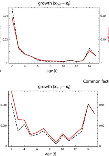
We estimated and visualized integration of growth from 2 to 4 years of age; the common factors of the subsequent growth periods closely resemble to the ones presented in Fig.3 and hence are not shown. Figure4a plots the covariance between the first pair of singular warps (between the shape features affected by common factor 1 as estimated from the growth from 2 to 4 years) for all one-year growth intervals within the sampled age range (from 2 to 3 years, 3–4, 4–5, etc.). The covariance decreases sharply and almost goes to zero at about 8 years of age; it rises again during puberty and decreases thereafter. This plot also shows the variance of common factor 1 during the different growth intervals. Apparently, covariance decrea-ses because variance decreadecrea-ses. The pleiotropic nature of the common factor remains unchanged but it ceases to vary across individual growth, probably because it stops con-tributing to development.
Instead of covariances of growth, we can also compute the usual cross-sectional covariances (covariance across individuals of the same age) between the shape features affected by common factor 1. Interestingly, even though
growth of these shape features is integrated and the underlying common factor varies during the first 6–8 years of postnatal growth (Fig.4a),cross-sectionalvariance and covariance decrease (Fig.4b). But how can the cross-sec-tional variance of the factor decrease, even though it varies during growth? The answer is given in Fig.5a: Growth (the shape difference xt?1-xt) is negatively correlated with
individual morphology (xt) till about 8 years of age. This
means that individuals with a high score for common factor 1 (relatively small face, long clivus) experience less than average growth of these features (relative facial size increases, relative clivus length decreases as compared to the average), and individuals with a low score experience more than average growth along this factor. Such a process of variance reduction during growth has been termed tar-geted growthor developmental canalization (e.g., Wadd-ington1942; Tanner1963; Debat and David2001). From 2 to 8 years of age, cross-sectional variance of common
factor 1 is halved; the individuals gain similar relative sizes of the face and the clivus, including a similar relative pharyngeal width.
The developmental dynamics of common factor 2 clearly differ from the dynamics of the first factor. Cross-sectional variance and covariance continuously increase (Fig.4d) even though variance and covariance of growth decrease during the first years of age (Fig.4c). Cross-sectional (co)variance increases because growth along common fac-tor 2 is uncorrelated with individual age-specific morphol-ogy—growth is not canalized (Fig. 5b). Variances and covariances thus accumulate during ontogeny.
The increasing variance of both common factors during early puberty reflects the massive variation in theonsetof puberty. After all individuals have reached puberty and experienced a growth spurt, variance decreases again. But such a reduction of variance usually is not interpreted as a canalization process.
Analysis 2: Comparing Integration Between Humans and Chimpanzees
In order to compare integration between the face and the cranial base in humans to that in chimpanzees, we used CT scans of 20 adult human individuals (10 males, 10 females from different human populations) from the sample used in Bookstein et al. (2003) and 22 adult chimpanzees (Pan troglodytes, most specimens of unknown sex) from the sample used in Neubauer et al. (2010). Additionally, we included two fossils with a preserved cranial base from the Bookstein et al. (2003) data set, the early modern human skull Mladecˇ I from central Europe (Czech Republic) and the South African Australopithecus africanus STS 5. The cranial base is represented by the four landmarks basion, dorsum sellae, sphenobasilare, and nasion, and the face by the five landmarks posterior nasal spine, nasospinale, prosthion, rhinion, and glabella (Fig. 6a). The assignment of nasion to the cranial base instead of to the face (or to both parts) is somewhat arbitrary, especially as glabella is assigned to the face. However, the presented results do not depend on these choices (see also the Discussion). The landmark configurations were superimposed by a single Procrustes registration.
After subtracting from each human individual the cor-responding sex average and projecting out allometry, we estimated common factors (scaled singular warps) from the residual shape coordinates as described above. The first common factor reflects variation in overall cranial length relative to cranial height, whereas the second common factor represents the size of the face and the anterior cranial base relative to the length of the clivus (Fig.6b, c). These two factors clearly resemble the factors estimated from the longitudinal sample above (Fig.3). They account for 93 %
Fig. 4 aCovariance between the first pair of singular warp scores (covariance between face and cranial base due to common factor 1) during one-year growth periods (individual shape differences between 2 and 3 years, 3 and 4 years, etc.), shown as ablack dashed line. Thered lineindicates the variance of common factor 1 in these growth intervals
(note the different scale at theright vertical axis).bCross-sectional variance (red line) and covariance (black dashed line) for common factor 1 across individuals of the same age.cVariance and covariance for common factor 2 during one-year growth periods.dCross-sectional variance and covariance for common factor 2 (Color figure online)
Fig. 5 Correlation of individual shape changes during one-year growth intervals with the morphology before growth ðCorðxtþ1
xt;xtÞÞplotted against age (t) for both common factors. A negative
correlation indicates targeted growth or canalization, because indi-viduals with a low score for this factor grow more than the average and individuals with a high score grow less
of summed squared covariances in the cross-sectional human sample.
Using these common factor estimates from the human sample, we computed scores along the factors (singular warp scores) both for humans and chimps. The scores were computed separately for the face and the cranial base. Note that we use the original human sample here, not the one corrected for sex and allometry, in order to investigate if average sex and species differences follow the integration pattern. Figure7b shows that—despite apparent mean shape differences—integration due to common factor 1 is similar in humans and in chimps: the point clouds are similarly oriented, i.e., one unit of shape change in the cranial base is associated with a similar amount of facial shape change in both species. Yet, var-iance (and thus also covarvar-iance) along this factor is much larger in humans than in chimpanzees. Mladecˇ I falls within the modern human distribution, whereas STS 5 clusters with the chimpanzees. The situation is different for common factor 2: In contrast to humans, chimpanzees are not integrated along the second common factor; both fossils are closer to the human than to the chimpanzee distribution. Human males and females completely over-lap for both factors.
Discussion
Olson and Miller coined the term ‘‘morphological inte-gration’’ with their 1958 book and raised a broader interest for this topic in the paleontological and biological com-munities. Yet, they never defined morphological integra-tion in their book (as pointed out, e.g., by Chernoff and Magwene 1999). As Olson and Miller, many subsequent authors referred to morphological integration either as the underlying developmental and functional causes or as the statistical pattern of phenotypic variances and covariances. We showed that net phenotypic covariances do not directly reflect the underlying developmental and genetic factors of integration, most importantly because covariances depend on the variance of pleiotropic factors in a sample, and multiple pleiotropic factors with opposite effects may partly cancel out. Like Cheverud (1996a,b), we thus used the term integration to denote the biological processes and properties leading to phenotypic covariance. The definition of integration by Hallgrimsson et al. (2009) as the ability to covary, rather than actual covariance, closely reflects this distinction.
The use of covariances to describe the relationship between phenotypic traits originates from early biometrics
a
b
c
Fig. 6 aMidsagittal landmarks on the cranial base (basion, dorsum sellae, nasion, sphenobasilare) and the face (posterior nasal spine, nasospinale, prosthion, rhinion, glabella) measured on CT scans of adult humans, chimpanzees, and two fossils. The first two singular
warps estimated from the human sample are visualized as common factors in (b) and (c). They clearly resemble the common factors in Fig.3, just the order is reversed
and from their role in predicting response to selection. But actual scientific models usually are not based on covari-ances, but on regressions (e.g., Bookstein in press). Regression quantifies the average effect of one variable onto another—how a change in one trait would alter another trait in the course of development or evolution—reflecting the typical reasoning in biology. Multivariate factors, such as Wright’s general factors or singular warps, can be interpreted as regressions of the variables on the (unmea-sured) factor score—they are models of how an underlying growth factor affects phenotypic traits (the path coefficients in Fig.1). When comparing integration between humans and chimps in Fig.7, we interpreted similar regression slopes between the singular warp scores as an indication of similar integration, regardless of the different covariances. Regressions and factor models describe the ability or pro-pensity of phenotypic traits to covary; the induced covari-ance depends on the sample varicovari-ance.
We reviewed different forms of integration (develop-mental integration, genetic integration, environ(develop-mental inte-gration) along with multiple other sources of phenotypic covariances, such as geometric and spatial dependences between the measurements. Developmental integration is the result of a very large number of developmental pro-cesses. The effect of single developmental factors can only be identified experimentally (see, e.g., the work by Hall-grimsson et al. on mice; HallHall-grimsson et al. 2004, 2006,
2009). Modern imaging techniques allow for the three-dimensional measurement of morphological features even during organogenesis and fetal development (e.g., Metscher
2009; Metscher and Mu¨ller2011). Based on morphometrics alone, it is impossible to specify how many genes or growth
processes actually contribute to an estimated common factor and the induced phenotypic covariance, but it is a well-known phenomenon that the vast array of genetic variation is ‘‘funneled’’ into a smaller set of pathways, which in turn influence a smaller set of developmental processes (Hall-grimsson and Lieberman 2008). Furthermore, it has been argued that structural and organizational integration at the morphological level determines the identity and homology of anatomical elements, regardless of the complex under-lying genetic and developmental networks (Mu¨ller and Newman 1999; Mu¨ller 2003). Careful studies of morpho-logical integration can model these few mediating processes and can compare them across age groups and across dif-ferent species. The heritable (additive genetic) part of the induced phenotypic variances and covariances is sufficient to predict short-term response to selection. Because exper-imental approaches are not possible in humans and primates, studies of morphological integration are a good alternative to investigate developmental integration in these taxa. Cranial Integration in Humans and Chimpanzees
We studied morphological integration between the cranial base and the face during postnatal human growth using 26 individuals of the longitudinal Denver Growth Study. This is a relatively small sample for reliably estimating vari-ances and covarivari-ances and it is probably no representative random sample, but we could still estimate and interpret two common factors (general factors in Wright’s termi-nology, or pleiotropic factors in the quantitative genetic language) underlying the integration between the cranial base and the face. These factors were estimated from
a
b
Fig. 7 Scores along the first two common factors, computed separately for the face and the cranial base (first two pairs of singular warp scores). Chimpanzees are shown as filledgray circles, male and female humans as filled andempty black circles, respectively. Along
common factor 1, humans and chimpanzees are similarly integrated but differ in variance (a), whereas chimpanzees are not as integrated along common factor 2 as humans are (b)
individual growth between 2 and 4 years of age, but the same two factors were also detectable from the other growth periods and even from the cross-sectional subs-amples. In the second analysis, the same two factors could be estimated from a different and very heterogenous sam-ple of 20 adult humans, even though number and position of the landmarks differed slightly across the two data sets. The first common factor reflects a large face together with a long anterior cranial base (the ‘‘roof’’ of the face) relative to the clivus (which is part of the middle cranial fossa), thus also determining the relative width of the pharynx. The face is under different developmental control than the brain and the basicranium, but facial length and the length of the anterior cranial base need to fit (‘‘growth counterparts’’; Enlow and Hans1996)—they are develop-mentally integrated. The anterior cranial base elongates in concert with the frontal lobes of the brain, reaching approximately 95 % of its adult length by the end of the neural growth period, but the more inferior portions of the anterior cranial base continue to grow as part of the face after the neural growth phase, forming the ethmomaxillary complex (Lieberman et al.2000). This common factor is of apparent functional relevance because of its effect on jaw size and on pharyngeal width. This is likely the reason why common factor 1 is canalized during postnatal ontogeny: the sample variance of common factor 1 is halved within six years of postnatal development.
The second common factor is a standard finding in cephalometrics: Relative height and length of anatomical elements are integrated within the cranium (dolichoce-phalic versus brachyce(dolichoce-phalic crania), where shorter faces are associated with a more flexed cranial base than longer faces (e.g., Enlow and Hans1996; Bookstein et al. 2003; Bastir and Rosas2004; Mitteroecker and Bookstein2008). Growth processes are integrated in this way throughout full postnatal development and the cross-sectional covariance between these shape aspects increases during ontogeny. This factor seems to be less developmentally canalized than common factor 1, probably because it is of no obvious functional relevance.
Using longitudinal data, we could study both cross-sectional integration and integration of growth itself, i.e., how cross-sectional variance and covariance is actually generated. The variance of common factor 1 during growth is much higher than the variance of common factor 2, and likewise, common factor 1 has a higher cross-sectional variance at age 2 than the second factor (cross-sectional variances of about 0.4 versus 0.3; Fig.4). But owing to the different developmental dynamics, the situation is reversed at age 16: Common factor 2 is three times more variable than common factor 1 in the cross-sectional sample of 16-year-olds. It is a common finding in cephalometrics that the ratio of overall length to height (our common factor 2)
is the most dominant pattern of variance and covariance apart from allometry (e.g., Bookstein et al. 2003; Bastir and Rosas 2004; Mitteroecker and Bookstein 2008).
In our second analysis, we compared integration between the face and the cranial base in cross-sectional samples of adult humans and chimpanzees. Basically the same two common factors result from this cross-sectional human sample as from the longitudinal X-ray sample (just in reversed order). Both humans and chimpanzees are similarly integrated regarding the overall length to height ratio of the face and the cranial base, but differ in the integration between facial size and anterior cranial base length. In humans, the face is positioned below the anterior cranial base and hence both parts are developmentally integrated. In chimpanzees, large parts of the face are more anteriorly positioned than the brain case, so that facial size and the length of the anterior cranial base are less inte-grated and almost uncorrelated in our sample. This is probably the reason why the average species difference between humans and chimpanzees—the evolutionary integration—along this common factor does not resemble the human integration pattern (Fig.7b). Evolutionary integration of length to hight ratios, by contrast, more closely resembles the common pattern of developmental integration in both species (Fig. 7a).
As we set out in the beginning, these insights are not derived from a formal mathematical model, nor are they based on biological experiments. They are based on the consilience of multiple lines of evidence: spatial statistical patterns (deformation grids), temporal statistical patterns (ontogenetic dynamics of variance and covariance), and qualitative biological models (both of development and function).
The Palimpsest
Most studies on integration and evolutionary quantitative genetics assess covariances in cross-sectional samples of adult individuals. It has been shown that cross-sectional variances and covariances continually change during development (e.g., Zelditch et al.2006; Hallgrimsson et al.
2007, 2009; Mitteroecker and Bookstein 2009). Hall-grimsson et al. (2007) used the metaphor of a medieval palimpsest to described the ontogeny of the adult covari-ance structure: Much like a reused scroll on which the shadows of the various texts accumulate over time, ‘‘the covariation structure of an adult skull represents the sum-med imprint of a succession of effects, each of which leaves a distinctive covariation signal determined by the specific set of developmental interactions involved’’ (p. 164). In our analysis we were able to show how variation in growth at different age stages contributes to the final pat-tern. We can thus add a further piece to the palimpsest
metaphor: Variation of growth processes can accumulate during ontogeny, whereas other growth processes are canalized so that cross-sectional variances and covariances decrease. Some text fragments on the palimpsest accumu-late over time, whereas others get (partly) erased in the course of ontogeny. Many, but not all growth processes varying in a population might be reflected in the adult covariance structure.
Acknowledgments We thank Mihaela Pavlicev and Fred Bookstein for stimulating discussions and helpful comments on the manuscript. We are grateful to Ekaterina Stansfield for loaning us the digitized Denver growth study data.
References
Armbruster, W. S., & Schwaegerle, K. E. (1996). Causes of covariation of phenotypic traits among populations.Journal of Evolutionary Biology, 9, 261–276.
Arnold, S. J., Bu¨rger, R., Holenhole, P. A., Beverly, C. A., & Jones, A. G. (2008). Understanding the evolution and stability of the G-matrix.Evolution, 62, 2451–2461.
Arnold, S. J., Pfrender, M. E., & Jones, A. (2001). The adaptive landscape as a conceptual bridge between micro- and macro-evolution.Genetica, 112-113, 9–32.
Arthur, W. (2002). The emerging conceptual framework of evolu-tionary developmental biology.Nature, 415(14), 757–764. Bastir, M., & Rosas, A. (2004). Facial heights: Evolutionary
relevance of postnatal ontogeny for facial orientation and skull morphology in humans and chimpanzees.American Journal of Physical Anthropology, 47,359–381.
Bastir, M., & Rosas, A. (2005). Hierarchical nature of morphological integration and modularity in the human posterior face. Amer-ican Journal of Physical Anthropology, 128(1), 26–34. Bastir, M., & Rosas, A. (2006). Correlated variation between the
lateral basicranium and the face: A geometric morphometric study in different human groups.Archives of Oral Biology, 51, 814–824.
Bastir, M., Rosas, A., Stringer, C., Manuel Cue´tara, J., Kruszynski, R., Weber, G. W., et al. (2010). Effects of brain and facial size on basicranial form in human and primate evolution.Journal of Human Evolution, 58(5), 424–431.
Berg, R. L. (1960). The ecological significance of correlation pleiades.Evolution, 14, 171–180.
Bogin, B. (1999).Patterns of human growth. Cambridge: Cambridge University Press.
Bonner, J. T. (1988).The evolution of complexity by means of natural selection. Princeton, NJ: Princeton University Press.
Bookstein, F. (1991). Morphometric tools for landmark data: Geometry and biology. Cambridge, UK: Cambridge University Press.
Bookstein, F. (1996). Biometrics, biomathematics and the morpho-metric synthesis. Bulletin of Mathematical Biology, 58(2), 313–365.
Bookstein, F. (1997). Landmark methods for forms without land-marks: Morphometrics of group differences in outline shape. Medical Image Analysis, 1(3), 225–243.
Bookstein, F. L. (in press). Reasoning and measuring: Numerical inferences in the sciences. Cambridge: Cambridge University Press.
Bookstein, F. L., Gunz, P., Mitteroecker, P., Prossinger, H., Schaefer, K., & Seidler, H. (2003). Cranial integration in Homo: Singular
warps analysis of the midsagittal plane in ontogeny and evolution.Journal of Human Evolution, 44(2), 167–187. Bulygina, E., Mitteroecker, P., & Aiello, L. C. (2006). Ontogeny of
facial dimorphism and patterns of individual development within one human population.American Journal of Physical Anthro-pology, 131(3), 432–443.
Chernoff, B., & Magwene, P. M. (1999). Morphological integration: Forty years later. In:Morphological integration, (pp. 319–354). Chicago: University of Chicago Press.
Cheverud, J. M. (1982). Phenotypic, genetic, and environmental morphological integration in the cranium. Evolution, 36, 499–516.
Cheverud, J. M. (1984). Quantitative genetic and developmental constraints on evolution by selection. Journal of Theoretical Biology, 110, 155–171.
Cheverud, J. M. (1988). A comparison of genetic and phenotypic correlations.Evolution, 42(5), 958–968.
Cheverud, J. M. (1989). A comparative analysis of morphological variation patterns in papionins.Evolution, 43, 1737–1747. Cheverud, J. M. (1996a). Developmental integration and the evolution
of pleiotropy.American Zoologist, 36, 44–50.
Cheverud, J. M. (1996b). Quantitative genetic analysis of cranial morphology in the cotton-top (Saguinus oedipus) and saddle-back (S. fuscicollis) tamarins.Journal of Evolutionary Biology, 9, 5–42.
Cheverud, J. M., Wagner, G. P., & Dow, M. M. (1989). Methods for the comparative analysis of variation patterns. Systematic Zoology, 38, 201–213.
Clausen, J., & Hiesey, W. M. (1960). The balance between coherence and variation in evolution.PNAS, 46(4), 494–506.
Debat, V., & David, P. (2001). Mapping phenotypes: Canalization, plasticity and developmental stability. Trends in Ecology & Evolution, 16(10), 555–561.
Enlow, D., & Hans, M. (1996). Essentials of facial growth. Philadelphia, PA: Saunders Company.
Falconer, D. S., & Mackay, T. F. C. (1996). Introduction to quantitative genetics. Essex: Longman.
Fisher, R. A. (1930). The genetical theory of natural selection. Oxford: Clarendon.
Galis, F., Van Dooren, T. J., Feuth, J. D., Metz, J. A., Witkam, A., & Ruinard, S., et al. (2006). Extreme selection in humans against homeotic transformations of cervical vertebrae. Evolution, 60(12), 2643–2654.
Gromko, M. H. (1995). Unpredictability of correlated response to selection: Pleiotropy and sampling interact. Evolution, 49, 685–693.
Gould, S. J. (1977).Ontogeny and phylogeny. Cambridge: Harvard University Press.
Gunz, P., & Harvati, K. (2007). The Neanderthal O` chignonO´: Variation, integration, and homology.Journal of Human Evo-lution, 52(3), 262–274.
Gunz, P., Mitteroecker, P., & Bookstein, F. L. (2005). Semilandmarks in three dimensions. In: D. E. Slice (Ed.),Modern morphomet-rics in physical anthropology(pp. 73–98). New York: Kluwer Press.
Gunz, P., Mitteroecker, P., Neubauer, S., Weber, G. W., & Bookstein, F. L. (2009). Principles for the virtual reconstruction of hominin crania.Journal of Human Evolution, 57(1), 48–62.
Haber, A. (2011). A Comparative Analysis of Integration Indices. Evolutionary Biology, 38,476–488.
Hallgrimsson, B., Brown, J. J., Ford-Hutchinson, A. F., Sheets, H. D., Zelditch, M. L., & Jirik, F. R. (2006). The brachymorph mouse and the developmental-genetic basis for canalization and mor-phological integration.Evolution & Development, 8(1), 61–73. Hallgrimsson, B., Dorval, C. J., Zelditch, M. L., & German, R. Z.