PDF hosted at the Radboud Repository of the Radboud University
Nijmegen
The following full text is a publisher's version.
For additional information about this publication click this link.
http://hdl.handle.net/2066/135143
Please be advised that this information was generated on 2017-12-05 and may be subject to
change.
Odyssey 2014:
The Speaker and Language Recognition Workshop 16-19 June 2014, Joensuu, Finland
NFI-FRITS: A forensic speaker recognition database and some first
experiments
David van der Vloed
1, Jos Bouten and David A. van Leeuwen
1,21
Netherlands Forensic Institute,
2Radboud University Nijmegen
{
d.van.der.vloed,d.van.leeuwen
}
@nfi.minvenj.nl
Abstract
In this paper we describe the collection of a speech data-base with forensically realistic data. It consists of speech material obtained from lawfully intercepted telephone conversations collected during police investigations. The speech material therefore is very similar to the kind we encounter in casework at the Netherlands Forensic Insti-tute. The database is augmented with metadata describ-ing language, accent, speakdescrib-ing style and acoustic con-ditions. A total of 604 speakers have been identified in 4188 conversation sides. After manual speaker attribu-tion using various forms of available metadata, the speech content has been anonymised by zeroing out fragments that might disclose the real identity of speakers. Addi-tional to the database description, this paper reports on some speaker recognition experiments using a commer-cially available forensic speaker recognition system. We can observe some effect of spoken language in terms of calibration, but overall the systems appears not too sensi-tive to accent or language.
1. Introduction
In this paper the Netherlands Forensic Institute’s Forensically Realistic Intercepted Telephone Speech database (NFI-FRITS) is presented, a database originating from recordings of tele-phone speech intercepted by Dutch law officials. It is similar in set-up to the AHUMADA 3 speech database [1] recorded in Spain by the Guardia Civil. The purpose of collecting the data-base is to obtain experience with automatic speaker recognition systems in a forensic setting, with the ultimate goal of support-ing evidence reportsupport-ing in forensic speaker comparison cases in a Bayesian framework. The intention is to share the database with public institutions; for more information the reader can contact the first author.
One of the conditions set by the law officials for using this material is that the finalised database has been anonymised, meaning that the metadata and audio can not contain any infor-mation that can disclose the real identity of a particular speaker. Therefore human annotators listened to all the recorded material and zeroed the audio fragments that contained such information. The annotators further provided some basic metadata as well, the single most important of which was (an encoded) speaker identity. The database contains forensically realistic material, i.e., audio data from real intercepted telephone speech, origi-nating from real police investigations. It is thus of the type that is frequently encountered in NFI casework, but not originating
from that source.
In forensic speaker comparison the general problem is to compare speech from a trace, typically a recording of speech containing incriminating evidence, to that of a suspect in terms of the identity of the speaker. In what is sometimes called the paradigm shift[2, 3] the aim is to present the result of the com-parison in a probabilistic way, and in analogy to the way DNA evidence is reported in court, the goal is to present the speaker comparison in terms of alikelihood ratio
r=P(speech|Hp, I) P(speech|Hd, I)
(1)
whereHpis theprosecutor’s hypothesis, stating that the
perpe-trator and suspect are the same person, andHdis thedefence’s
hypothesis, stating that the perpetrator is not the same person as the suspect.1 Important to note is the specification of other
information, or circumstances, in the case, specified asI that are conditioning the probabilities in the numerator and denom-inator in exactly the same way. Thus, the likelihood ratio only considers the likelihood of the hypotheses, and nothing else. The ‘speech’ in (1) represents all available speech material rel-evant to the case, i.e., both the suspect reference recording and the questioned recording (the trace). The log of the likelihood ratio
`= logr (2)
is known as the ‘weight of evidence’ [4] and has a long his-tory dating back to Turing in 1941. The log likelihood ratio has the nice property that different, independent, pieces of evidence are additive, and in this sense can be metaphorically viewed as items that can be put on the weighing scales of the Goddess of Justice [4].
In recent years a growing understanding of a procedure for producing likelihood ratios in case work has emerged. Orig-inally, attempts were made to estimate the probability den-sity functions (PDFs) similar to numerator and denominator in (1) [5,6], but later it was realised that the comparison score of an automatic speaker recognition system can be used directly in a score-to-likelihood ratio function that is learned using empirical data [2, 7–14], a process known ascalibration. Either way, the circumstances of the caseIshould be reflected in the data used to either directly estimate the PDFs or the empirical data that is used in the calibration process. If there are circumstancesI
for which it is linguistically or acoustically plausible that they influence the comparison value of a speaker recognition sys-tem, then the same linguistic or acoustic conditions should be applied to the data used for calibration. Well designed and pop-ular databases used in automatic speaker recognition research
1The defence hypothesis can be more specific than that, as long as it
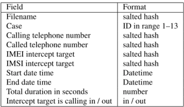
Table 1: Metadata provided with the raw recording data. ‘Date-time’ is a format specified as YYYY-MM-DD HH:MM:SS which can be sorted lexicographically.
Field Format
Filename salted hash Case ID in range 1–13 Calling telephone number salted hash Called telephone number salted hash IMEI intercept target salted hash IMSI intercept target salted hash Start date time Datetime End date time Datetime Total duration in seconds number Intercept target is calling in / out in / out
such as Switchboard [15, 16] and Mixer [17] do not cover the same circumstances as found in forensic case material, in terms of language, speaking style, quality, etc. In forensic speech databases such as NFI-FRITS, AHUMADA [1], GFS1.0 cor-pus [18] and NFI-TNO [19] these circumstances are covered to some extent, and by providing metadata it is possible to make a selection representingIin (1).
After presenting a description of the NFI-FRITS database in Section 2, this paper reports some experiments on a smaller sub-set of the database containing Turkish speakers in Section 3. This allows us to study circumstancesIin Section 4 where the trace contains speech in this language, and we can even study cases where the suspect reference recording is spoken in a dif-ferent language: Dutch, but with a Turkish accent.
2. Description of Database
2.1. Speech material
The NFI-FRITS (recordings of telephone speech intercepted during real police investigations) consists of Dutch, Moroccan Arabic, Berber and Turkish speech material. This material was obtained to facilitate research on data typically encountered in forensic practice, much like the data used by [1, 18, 19]. To comply with legal regulations, the data was anonymised by ze-roing speech that contained information traceable to an individ-ual. Annotators native in the relevant languages were hired to perform this task. The NFI-FRITS consists of 4188 speech files with speech from 604 different speakers.
2.2. Data processing
The raw data were provided as 2-channel, 8 kHz 8 bit A-Law encoded waveform files and in the majority of recordings both ends of the conversation are recorded in separate channels. These files came with some metadata, such as the two telephone numbers involved in the telephone call, IMEI numbers and case names. These can be found in Table 1.
The audio files were first split in two single channel files (a and b), expanded to 8kHz, 16 bit PCM and stored in a database, along with the provided metadata. The native human annota-tors listened to all recordings and identified speaker names (of the type ‘John,’ ‘John’s girlfriend,’ ‘guy from the pizza place’), determined a gender for the speaker (male/female) and then as-signed single channel files from the database to that speaker. In this process, information like the telephone number, the case, and the spoken content of the speech file was taken into
ac-Table 2: Metadata provided by the annotators Field Format/value
Speaker ID 6 digit number
Language ID ID in range 1–12, see Table 4 Language proficiency native, good, poor
Loud sounds yes/no
Background music No / short / long
Audible noise No / weak / intermediate / strong Formal conversation Yes / No
Age group Adult / very young / very old Conversation type Dialogue / monologue Background speakers Yes / No
In motorised vehicle Yes / No Strong reverberation Yes / No Emotional speech No / short / long Whisper No / short / long Raised voice No / short / long Regional speech No / Yes Remarks Plain text
count. Subsequently, the audio was listened to again and all the speech that contained information that could possibly identify an individual was removed by setting all the digital sample val-ues to zero in these fragments within the audio file. Addition-ally, other metadata was added by the annotators, only based on their listening, like spoken language, language proficiency, a broad indication of the age of the speaker and so forth. A complete list can be found in Table 2. This process was carried out until about five recordings were assigned to an individual speaker, after which a new speaker was selected and the pro-cess was repeated.
In total, 604 different speakers were identified (117 female / 427 male) and 4188 conversation sides were assigned to these speakers (1068 female / 3120 male).
After this phase all the data were listened to again by a forensic speech scientist. The speaker assignment of the record-ings was verified by listening. During this operation back-ground sounds were marked for exclusion by marking all times of intervals to be excluded. Thus, call tones, periodic back-ground sounds, backback-ground speakers, crosstalk, messages from the mobile phone operator, etc. can be automatically excluded. The time interval marking makes it possible to generate a ver-sion of the database that contains audio that resembles edits as typically used in case work. However, due to the large number of files and the limited available resources, it is possible that the end result still contains some audio that would have been edited out in case work.
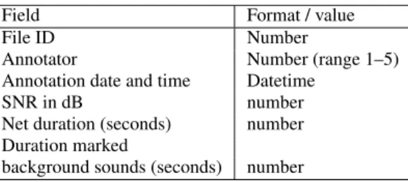
The last step was to anonymise the metadata, by deleting or by replacing it with salted hashes or ID-numbers. The meta-data replaced by hashes are: ‘calling telephone number,’ ‘called telephone number,’ ‘IMEI’ and ‘IMSI.’ The metadatum that was replaced by an ID is ‘case name.’ Speaker names were deleted. Some new metadata were generated, which can be found under in Table 3.
2.3. Speaker identities
Due to the origin of the data there is no absolute certainty about speaker identities assigned by the annotators. However, they based their choice on names and other information about the speakers they gathered by listening, layman speaker recognition and the fact that two speech samples coming from the same
Table 3: Semi-automatically generated metadata Field Format / value
File ID Number
Annotator Number (range 1–5) Annotation date and time Datetime
SNR in dB number Net duration (seconds) number Duration marked
background sounds (seconds) number
telephone number are very likely to be from the same speaker, especially if it is a mobile phone number. The annotators were instructed to ignore the audiofiles about which they had doubts regarding speaker identity. Furthermore, the speaker identity was verified by another annotator who listened to the material, and when there was doubt about speaker identity, the audio file was discarded. Speaker identity is thus no absolute truth, but rather a truth by proxy.
The speakers are all people that were recorded in lawfully intercepted telephone calls. It is likely that a speaker was not aware that he or she was recorded at the time of speaking, al-though since precise circumstances of the investigations are un-known, and given the reason for interception and the potentially criminal activities of the speakers, this is not certain.
2.4. Recordings
2.4.1. Number of recordings per speaker
The aim of the database was to collect five recordings per speaker. However, some speakers in the database have more recordings associated with them, because initially no aim was set. Because of concerns that the total number of speakers in the recordings would become too low within the conditions of the allotted resources for producing the database, the aim was first set at ten, and later that number was lowered to five. Con-versely, some speakers have less than five recordings assigned to them. This is because, during the annotation procedure, there sometimes was no new case material available and hence the annotators were instructed to continue with the case, aiming for speakers with three or four recordings. Finally, the annotator verifying the material could also remove recordings assigned to a speaker.
2.4.2. Duration of recordings
The gross duration of the recordings was stored with the record-ings, defined as the entire duration of the provided audio file. The minimum gross duration was set at 30 seconds and the max-imum duration was set at 600 seconds. This maxmax-imum duration was determined in the course of the project so that the anno-tators would not spend too much time and effort on a single recording.
In total 165 hours of speech has been annotated in 4188 segments. The histogram of duration is shown in Figure 1, the mean segment duration after automatic energy-based speech ac-tivity detection is 142 seconds. On average, 3.85 s of speech (2.7 %) was nulled as a result of the anonymisation procedure. 2.4.3. Languages
The languages included in this database are Dutch (nld), Moroc-can Arabic (ary), Tarifit (rif) and Turkish (tur). These languages
Segment duration duration (s) Frequency 0 100 200 300 400 500 0 100 200 300 400 500 duration gross after SAD
Figure 1: A histogram of a segment duration before and after automatic speech activity detection (SAD).
were chosen as the target languages because these are the lan-guages that occur most frequently in case work at the NFI. Not unrelated, these are the languages that are most frequent in the provided material. Attempts to gather recordings in other lan-guages would have become very difficult, since this would in-volve a lot of effort spent on just trying to find the recordings in those languages.
The actual values in the language field in the database are a bit more complex, so that the language field would be a bit more informative about the speaker and his or her background. The possible values are given in Table 4, together with the statistics of language proficiency as judged by the native annotators.
The ‘Dutch by an hareai speaker’ language fields were used for recordings containing ethnolectic Dutch. The Mix-languages were used when multiple Mix-languages were used by the same speaker in a single recording.
3. Experimental design
In order to give an impression of how this speech database can be used for forensic speaker recognition research we have con-ducted an experiment with an automatic speaker recognition system. The full database is quite heterogeneous in terms of speaker population and spoken language, so we decided to carry out a first characterisation experiment using a preliminary sub-set of the data.2From the entire database, we selected segments
(i.e., conversation sides in NIST SRE 2006 parlance) in which either Turkish (“tur”), Dutch with a Turkish accent (“nld-t”) or a mix of Dutch and Turkish (“nld/tur”) was spoken. This selec-tion resulted in 60 distinct speakers in 534 segments, approxi-mately 10 % of NFI-FRITS. For each speaker, the available ments were divided in equal numbers over ‘train’ and ‘test’ seg-ment classes, where in the case of an odd number of segseg-ments the ‘train’ segment class received one more than the ‘test’ class. This procedure resulted in 211 training segments (58 speakers)
Table 4: Distribution of spoken languages and proficiency
Language —abbreviation in this paper Language proficiency Total native good poor
Dutch 2416 62 5 2483
Turkish —tur 472 27 - 499
Moroccan Arabic 142 49 - 191
Dutch by Morrocan speaker 20 184 1 205
Berber (Tarifit) 116 - - 116
Dutch by Turkish speaker —nld-t 60 296 10 366 Dutch by Caribbean speaker (Surinam/Dutch Antilles) 37 - - 37 Mix of Arabic and Dutch 71 13 - 84 Mix of Arabic and Berber 3 1 - 4 Mix of Berber and Dutch 17 2 - 19 Mix of Dutch and Turkish —nld/tur 16 120 2 138
Other 27 13 6 46
and 323 test segments (59 speakers). The imbalance is because the speaker recognition system employed has default minimum requirements for training duration (30 sec) and signal-to-noise ratio (10 dB).
The automatic speaker recognition system computes scores (or likelihood ratios) for all train segments vs. all test segments, resulting in 68 153 trials. These can further be classified accord-ing to train/test spoken language accordaccord-ing to Table 5.
In one operational condition the speaker recognition sys-tem can specify ‘reference population’ speech material for score normalisation and calibration purposes. For this, we used one segment for each of 44 speakers chosen outside the test data-base, roughly equally distributed over the three language condi-tions.
3.1. Speaker recognizer conditions
We used a commercially available automatic speaker recogni-tion system in this research3, we therefore know little details about features and background training data. Its engine is a modern i-vector system with PLDA scoring, and can operate in two modes: it can just produce an uncalibrated PLDA score, or it can produce a calibrated likelihood ratio that can be used in forensic evidence reporting. For the latter, the system needs a collection of utterances from a reference population, which can be seen as representative speakers of the alternative hypothe-sisHd.
3.2. Spoken language conditions
Using different cuts of the test set according to Table 5, we can investigate the influence of spoken language on a speaker recog-nition trial. We can analyse results per language/accent, or look across-language/accent effects.
3.3. Normalisation for distribution of trials over speakers
Even though the collection of segments per speaker was steered towards a fixed number of segments per speaker, the availability of the data in the various police investigation cases still skewed this distribution, see Figure 2. To compensate for the different amounts of trials available per speaker, we apply trial weighting in the performance analysis steps. The details of trial weighting are described in an earlier paper [20], where the influence of different amounts of trials for different conditions in NIST
SRE-3Agnitio Batvox Eval version 4
2008 was equalised. If the number of trials involving speaker
s1ands2in hypothesisHis denoted byN(s1, s2, H), then the
steps in the DET plot [21] become dependent on the speakers involved: ∆PFA(s1, s2) = 1 NsN(s1, s2, Hd) , (3) ∆Pmiss(s) = 1 NsN(s, s, Hp) , (4)
whereNs is the number of target speakers whose influence is
equalized. Similar expressions can be deduced [20] for perfor-mance metrics such asCllrandCllrmin[7]. We used version 0.8
of the R librarysretoolsfor the trial weighting analysis [22]. We believe [23] applied the same idea to speakers, by “averag-ing DET plots . . . for every target / non-target speaker pair,” which is mathematically equivalent. In our formulation, each trial is weighted inversely proportional to the contingency table of trials for the factors train speaker ID and test speaker ID.
4. Results
4.1. Equalization
In a first experiment we analyse the effect of the trial weight-ing. In Figure 3 we show the effect on the DET-plot. We can observe that for this data set the curve becomes more ragged, which is probably caused by speaker combinations with rela-tively few mutual trials being weighted quite heavily in the DET (cf. (3)–(4)). The contingency table, being a product of two sim-ilarly skewed speaker distributions as in Figure 2, is even more skewed, with frequencies ranging from 1 to 726. A second ob-servation is that for this data set the equal error rateE=is lower
when speaker trial weighting is in effect. In the following, we will use speaker weighting in the analysis.
4.2. Reference population and calibration
In the next experiment, we compare the effect of the reference population to the recognition performance. In Figure 4 we com-pare the DET plot for the condition without reference popula-tion to that with reference populapopula-tion, where in the latter case we show both the ‘raw scores’ and the ‘likelihood ratio’ output. The two curves with a reference population are not identical, meaning that the calibration is a non-monotonic function of the scores. However, there is no qualitative difference in discrimi-nation performance for the three curves.
Table 5: Target / non-target trial counts for the various combinations of spoken language/accent in the experimental data set. train\test tur nld-t nld/tur total
tur 762 / 23304 332 / 12520 61 / 3719 1155 / 39543 nld-t 241 / 9500 480 / 4722 46 / 1484 767 / 15706 nld/tur 116 / 6378 82 / 3386 90 / 930 288 / 10694 total 1119 / 39182 894 / 20628 197 / 613 2210 / 65943
number of segments per speaker available
number of segments per speaker
Frequency 0 10 20 30 40 50 0 5 10 15 20 25 30
Figure 2: The distribution of the number of available segments per speaker, for the experimental selection of the database.
Effect of equalizing trial counts in analysis
false alarm probability (%)
miss probability (%) 0.1 0.5 2 5 10 20 40 0.1 0.5 2 5 10 20 40 raw counts equalized
Figure 3: The effect of equalising the weight of different speak-ers, by compensating for their relative frequency. The recog-nizer is employed in the condition without reference population.
Comparison of recognizer condition
false alarm probability (%)
miss probability (%) 0.1 0.5 2 5 10 20 40 0.1 0.5 2 5 10 20 40 without population with popularion, raw scores with polulation, likelihood ratios
Figure 4: The effect of the condition of the speaker recognizer, with/without reference population, raw scores / log likelihood ratios.
If we consider not only discrimination but also calibration performance, there is quite a difference between the conditions. In Table 6 we illustrate the performance in terms ofCllr, a
calibration-sensitive general performance metric for likelihood ratios [7]. In the first line in the table, it is not really fair to compare Cllr to Cllrmin, because under this condition we take
raw scores, which are not calibrated. Cllr measures
calibra-tion, essentially telling us to what extent the scores behave like calibrated log-likelihood-ratios, and we know that raw recogni-tion scores—even when obtained by PLDA log likelihood ratio scoring—still need a calibration step. Specifying a reference population has a positive effect onCllr, but the value is still
quite far from the minimum attainable valueCmin
llr given the
discrimination performance. Finally, the LLR values`(2) as produced by the recognizer result in aCllrquite close toCllrmin,
so we can conclude that the calibration is quite good. From now on we will work with the LLR scores from the recognizer con-dition where we used a reference population (cf, Section 3.1).
In Figure 5 the densities of`for target and non-target trials are shown. Essential to good calibration performance is that the log of the ratio of the red and blue curves is equal to the value on thex-axis, for all LLRs [24]. One can observe that where the lines cross, this is the case: this happens at`= 0. Cumulative densities are known as “Tippet plots” [5, 25] and are frequently shown in forensic science literature. These cumulative densities are essentially1−PFA andPmiss, and therefore contain the
−20 −10 0 10 0.00 0.04 0.08 0.12 PDFs LLR Density targets non−targets
Figure 5: The probability density functions for target and non-target LLRs from the recognition system.
Table 6: Performance metrics for the three conditions shown in Figure 4. We used speaker equalisation for the analysis. RP: reference population, LLR: log likelihood ratios
Condition score Cllr Cllrmin E=
without RP raw 1.202 0.407 12.2 % with RP raw 0.724 0.402 12.1 % with RP LLR 0.447 0.405 12.3 %
same information as a ROC or DET plot, except that in these plots the LLR values are implicit. Sometimes the proportion of non-target trials with` >0is referred to as the ‘misleading evidence’ [26], but of course for calibrated`this is just the equal error rateE=.
4.3. Effect of language
We can now investigate the effect of spoken language on the recognition performance. From Table 5 we can see that our experimental sub-set from the NFI-FRITS database allows for many different train/test combinations of language. It is impor-tant to choose the conditions the same, under whichHpandHd
trials are selected, when computing likelihood ratios. For in-stance, when comparing a suspect speaking Turkish (‘tur’) with a perpetrator speaking Dutch with a Turkish accent (‘nld-t’) this language combination should be considered as part of the cir-cumstancesIin the likelihood ratio (1). Hence for a meaning-ful experiment we should take both target and non-target trials using the same language conditioning.
4.3.1. Effect of language/accent mix
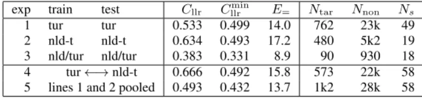
First we condition on the language/accent mix, as shown in the top three lines in Table 7, corresponding to diagonal entries in Table 5. We might conclude that calibration (Cllr−Cllrmin) is
more problematic for the Turkish-accented Dutch than for na-tive Turkish speakers. The discrimination performance (Cllrmin,
E=) seems to vary quite a bit, however, the number of speakers
Ns and available target and non-target trials (NtarandNnon)
aren’t very high and consequently DET curves are quite ragged.
4.3.2. Cross language effects
Another condition worth studying is the effect of different lan-guages spoken in train and test. In the fourth line of Table 7 we have tested segments spoken in Turkish vs. segments spoken in Dutch with a Turkish accent. Hereby we have pooled trials with Turkish as either train or test language. The discrimination performance (E=) is not really different from conditions with
the same language for train and test (cf. lines 1 and 2 from the table), but the calibration (Cllr−Cllrmin) suffers. A fair
com-parison of this condition is perhaps to the performance obtained when the trials of lines 1 and 2 are pooled. We have shown this in the 5th line of the table, which indicates remarkably good calibration performance. It may seem counterintuitive that the pooling of two trial sets gives rise to better performance than that of the sets individually, but it can be seen as an effect of the trial weighting procedure that we employ.
5. Discussion and conclusions
On the one hand, the experiments in the previous section are examples of investigations that can be performed with a multi language and accented forensic database such as NFI-FRITS. On the other hand, it shows the limitations in the way we com-pare conditions of the speaker comparison, because different conditions will select different sections of the data with differ-ent speakers and differdiffer-ent numbers of speakers. The focus of this research is the methodology of using data from the data-base rather than characterisation of the absolute performance of the recognizer under different circumstances.
In the introduction we mentioned that the metadata in NFI-FRITS can be used to select circumstancesIrelevant to a foren-sic case. By selecting Turkish speakers in Section 3 we simulate such conditions. Then in Section 4 we used a further condition-ing to investigate if there are major performance differences in speaker recognition for spoken language (native Turkish, Dutch or a language mix), and the results are that we observe a similar effect to what has been reported earlier [9], namely that in gen-eral discrimination performance does not vary a lot with spoken language, but that there is a larger effect in terms of calibration performance.
We have not conducted a statistical significance test in the analysis of language effects. Apart from statistical tests for de-tection costs [27, 28] we are not aware of such an analysis for the measuresE=,CllrandCllrmin. The speaker-equalised trial
weighting we use (cf. (3) and (4)) further complicates such a rigorous analysis. We therefore limit ourselves to the more qualitative remark that when we take our test data to be more specific to the case at hand, the number of available speakers, segments and trials from the database diminishes rapidly, with a much more ragged DET curve and larger uncertainties in per-formance characteristics.
One might be concerned that the discrimination perfor-mance (E= ≈ 12 %) is not high enough to be used in Court.
However, as can be seen from Figure 5, the expected value for the LLR in the case ofHpis about 5, which corresponds to a
LR of about 150. Depending on the circumstances of the court case, this can be quite an informative value.
With the recording and annotation of NFI-FRITS we hope to have provided an infrastructure for investigating the
appli-Table 7: The performance of the recognizer’s log-likelihood-ratio scores when operating with reference population, conditioned by language/accent mix.
exp train test Cllr Cllrmin E= Ntar Nnon Ns
1 tur tur 0.533 0.499 14.0 762 23k 49 2 nld-t nld-t 0.634 0.493 17.2 480 5k2 19 3 nld/tur nld/tur 0.383 0.331 8.9 90 930 18 4 tur←→nld-t 0.666 0.492 15.8 573 22k 58 5 lines 1 and 2 pooled 0.493 0.432 13.7 1k2 28k 58
cation of automatic speaker recognition systems to forensic speaker comparison. With the annotation of a number of lin-guistically and acoustically relevant parameters the database can be used to select calibration material relevant to a particu-lar case. This allows validation of the use of automatic speaker recognition systems for forensic speaker comparison.
6. References
[1] Daniel Ramos, Joaquin Gonzalez-Rodriguez, Javier Gonzalez-Dominguez, and Jose Juan Lucena-Molina, “Addressing database mismatch in forensic speaker recog-nition with Ahumada III: a public real-casework database in Spanish.,” inProc. Interspeech, 2008, pp. 1493–1496. [2] Daniel Ramos-Castro, Joaqu´ın Gonz´alez-Rodr´ıguez, and
J. Ortega-Garcia, “Likelihood ratio calibration in a trans-parent and testable forensic speaker recognition frame-work,” in Proc. Odyssey 2006 Speaker and Language Recognition Workshop, 2006.
[3] Joaquin Gonzalez-Rodriguez, Phil Rose, Daniel Ramos, Doroteo T. Toledano, and Javier Ortega-Garcia, “Emu-lating DNA: Rigorous quantification of evidential weight in transparent and testable forensic speaker recognition,” IEEE Transactions on Audio, Speech and Language Pro-cessing, vol. 15, no. 7, pp. 2104–2115, September 2007. [4] I. J. Good, Bayesian Statistics 2, chapter Weight of
Evi-dence: A Survey, pp. 249–270, Elsevier Science Publish-ers, 1985.
[5] Didier Meuwly and Andrzey Drygajlo, “Forensic speaker recognition based on a Baysian framework and gaussian mixture modelling (GMM),” in2001, a speaker Odyssee, June 2001, pp. 145–150, Crete.
[6] C.G.G. Aitken and D. Lucy, “Evaluation of trace evidence in the form of multivariate data.,” Applied Statistics, pp. 109–122, 2004.
[7] Niko Br¨ummer and Johan du Preez, “Application-independent evaluation of speaker detection,” Computer Speech and Language, vol. 20, pp. 230–275, 2006. [8] Daniel Ramos, Forensic Evaluation of the Evidence
Us-ing Automatic Speaker Recognition Systems, Ph.D. thesis, Universidad Autonoma de Madrid, November 2007. [9] Niko Br¨ummer, Luk´aˇs Burget, Jan ˇCernock´y, Ondˇrey
Glembek, Frantiˇsek Grezl, Martin Karafi´at, Pavel Matˇejka, David A. van Leeuwen, Petr Schwarz, and Al-bert Strassheim, “Fusion of heterogeneous speaker recog-nition systems in the STBU submission for the NIST speaker recognition evaluation 2006,” IEEE Transactions on Speech, Audio and Language Processing, vol. 15, no. 7, pp. 2072–2084, 2007.
[10] Daniel Ramos-Castro, Joaquin Gonzalez-Rodriguez, and Javier Ortega-Garcia, “Likelihood ratio calibration in a transparent and testable forensic speaker recognition framework,” in Proc. Odyssey 2008: The Speaker and Language Recognition Workshop, 2008.
[11] Daniel Ramos, Javier Franco-Pedroso, and Joaquin Gonzalez-Rodriguez, “Calibration and weight of the ev-idence by human listeners. the ATVS-UAM submission to NIST human-aided speaker recognition,” in Proc. ICASSP. 2011, pp. 5908–5911, IEEE.
[12] Miranti Indar Mandasari, Rahim Saeidi, Mitchell McLaren, and David A. van Leeuwen, “Quality measure functions for calibration of speaker recognition system in various duration conditions,” IEEE Transactions on Au-dio, Speech, and Language Processing, vol. 21, no. 11, pp. 2425–2438, Accepted for publication 2013.
[13] Milou van Dijk, Rosemary Orr, David van der Vloed, and David van Leeuwen, “A human benchmark for automatic speaker recognition,” in Proc. of the 1st International Conference Biometric Technologies in Forensic Science, Nijmegen, 2013, pp. 39–45.
[14] Geoffrey Stewart Morrison, “Tutorial on logistic-regression calibration and fusion:converting a score to a likelihood ratio,”Australian Journal of Forensic Sciences, vol. 45, no. 2, pp. 173–197, 2013.
[15] J. J. Godfrey, E. C. Holliman, and J. McDaniel, “Switch-board: telephone speech corpus for research and develop-ment,” inProc. International Conference on Acoustics, Speech, and Signal Processing (ICASSP), 1992, pp. 517– 520.
[16] David Graff, Kevin Walker, and Alexandra Canavan, “LDC Switchboard II phase 2,” 1999, Catalog ID LDC99S79.
[17] Christopher Cieri, Linda Corson, David Graff, and Kevin Walker, “Resources for new research directions in speaker recognition: The mixer 3, 4 and 5 corpora,” inProc. In-terspeech, Antwerp, 2007.
[18] T. Becker, “Automatic forensic voice comparison (au-tomatischer forensischer stimmenvergleich),” inThe Jour-nal of Speech Language and the Law, 2012, vol. 19, pp. 291–294.
[19] David A. van Leeuwen and Jos S. Bouten, “Results of the 2003 NFI-TNO forensic speaker recognition evaluation,” inProc. Odyssey 2004 Speaker and Language recognition workshop. June 2004, pp. 75–82, ISCA.
[20] David A. van Leeuwen, “Overall performance metrics for multi-condition speaker recognition evaluations,” in Proc. Interspeech, Brighton, September 2009, pp. 908– 911, ISCA.
[21] Alvin Martin, George Doddington, Terri Kamm, Mark Or-dowski, and Mark Przybocki, “The DET curve in assess-ment of detection task performance,” inProc. Eurospeech 1997, Rhodes, Greece, 1997, pp. 1895–1898.
[22] David A. van Leeuwen, “SRE-tools, a software package for calculating performance metrics for NIST speaker recognition evaluations,”http://sretools. googlepages.com/, 2008.
[23] George Doddington, “The effect of target/non-target age difference on speaker recognition performance,” inProc. Odyssey 2012: The Speaker and Language Recognition Workshop, Singapore, June 2012, ISCA.
[24] David A. van Leeuwen and Niko Br¨ummer, “The distri-bution of calibrated likelihood-ratios in speaker recogni-tion,” inProc. Interspeech. ISCA, 2013, pp. 1619–1623. [25] C. F. Tippet, V. J. Emerson, M. J. Fereday, F. Lawton,
A. Richardson, L. T. Jones, and S. M. Lampers, “The evidential value of the comparison of paint flakes from sources other than vehicles,” Journal of the Forensic Sci-ence Society, vol. 8, pp. 61–65, 1968.
[26] Richard Royall, “On the probability of observing mislead-ing statistical evidence,”Journal of the American Statisti-cal Association, vol. 59, no. 451, pp. 760–768, 2000. [27] Samy Bengio and Johnny Mari´ethoz, “A statistical
significance test for person authentication,” in Proc. Odyssey 2004 Speaker and Language recognition work-shop, Toledo, Spain, 2004.
[28] David A. van Leeuwen, Alvin F. Martin, Mark A. Przy-bocki, and Jos S. Bouten, “NIST and NFI-TNO evalua-tions of automatic speaker recognition,”Computer Speech and Language, vol. 20, pp. 128–158, 2006.