Universitat Politècnica de Catalunya (UPC) - BarcelonaTech
Facultat d’Informàtica de Barcelona (FIB)
Treball Final de Grau
Grau en Enginyeria Inform`
atica (GEI)
Enginyeria de Computadors
Improving nanos6 dependency subsystem
David Álvarez Robert
Directors:
Vicenç Beltran Querol
([email protected])Eduard Ayguadé Parra
([email protected])Computer Architecture Department (DAC)
Abstract
The OmpSs-2 programming model extends the basic dependency model of OpenMP with advanced features such as weak dependencies and dependencies over non-contiguous memory regions. These features also work across different task-nesting levels, provid-ing a general and fine-grained synchronization mechanism. In general, these advanced features simplify the parallelization of complex applications and also improve perfor-mance. However, the current implementation of the data dependency subsystem in the Nanos6 runtime is complex and thus difficult to optimize for certain use cases. In this work, a new alternative implementation of the dependency subsystem aiming to provide a subset of the current features but focusing instead in performance and simplicity is designed, developed and evaluated. Additionally, a mechanism to switch between both implementations at execution time is also added to Nanos6.
Resum
El model de programaci´o OmpSs-2 amplia el model b`asic de depend`encies d’OpenMP amb caracter´ıstiques avan¸cades com depend`encies weak i en regions de mem`oria no contig¨ues. Aquestes caracter´ıstiques tamb´e funcionen a trav´es de diferents nivells de parentesc entre tasques, proporcionant un mecanisme de sincronitzaci´o general i de gra fi. En el cas general, aquesta funcionalitat avan¸cada simplifica la tasca de paral·lelitzar programes complexos i en millora el rendiment. No obstant aix`o, la implementaci´o ac-tual del sistema de depend`encies a la llibreria Nanos6 ´es complexa i per tant dif´ıcil d’optimitzar per a certs casos. En aquest treball es dissenya, desenvolupa i avalua una nova implementaci´o alternativa del sistema de depend`encies, amb l’objectiu de propor-cionar un subconjunt de les caracter´ıstiques actual per`o centrant-se en el rendiment i la simplicitat. Addicionalment, s’incorpora a la llibreria un mecanisme per canviar entre ambdues implementacions en temps d’execuci´o.
Table of Contents
1 Introduction . . . 1
1.1 Motivation . . . 1
1.2 Actors . . . 2
2 State of the art . . . 3
2.1 Parallel programming models . . . 3
2.1.1 OpenMP . . . 3
2.1.2 OmpSs and OmpSs-2 . . . 4
2.1.3 Influence in OpenMP . . . 4
2.2 Data dependencies . . . 5
2.3 OmpSs-2 dependency model . . . 6
3 Scope . . . 9
3.1 Goal . . . 9
3.2 Requirements . . . 9
3.3 Scope . . . 9
3.4 Risks . . . 10
3.4.1 Deviation of the project plan . . . 10
3.4.2 Introducing bugs to the runtime . . . 10
3.4.3 Compilation and test times . . . 11
3.4.4 Result variance . . . 11
4 Methodology . . . 12 4.1 Time management . . . 12 4.2 Progress tracking . . . 12 4.3 Validation . . . 12 4.4 Final result . . . 13 5 Project plan . . . 14 5.1 Tasks . . . 14 5.1.1 Project management . . . 14 5.1.2 Runtime analysis . . . 15 5.1.3 Correctness tests . . . 15 5.1.4 Initial implementation . . . 15 5.1.5 Optimization . . . 15 5.1.6 Evaluation . . . 16 5.1.7 Thesis writing . . . 16 5.2 Timing . . . 16 5.3 Task dependencies . . . 17 5.4 Resources . . . 17 5.4.1 Hardware . . . 17 5.4.2 Software . . . 18 5.4.3 Human resources . . . 19 5.4.4 Spaces . . . 19
5.5 Workarounds and action plan . . . 19
5.6 Gantt diagram . . . 20 5.7 Deviations . . . 21 6 Economic management . . . 22 6.1 Direct costs . . . 22 6.1.1 Human resources . . . 22 6.1.2 Software . . . 22 6.1.3 Hardware . . . 23 6.2 Indirect costs . . . 23
6.3 Final budget . . . 24 6.4 Risk management . . . 25 7 Sustainability . . . 26 7.1 Economic dimension . . . 26 7.2 Social dimension . . . 27 7.3 Environmental dimension . . . 27
8 Analyzing the runtime and writing tests . . . 29
8.1 Compiling the runtime . . . 29
8.2 Writing and compiling OmpSs-2 programs . . . 30
8.3 Runtime architecture . . . 31
8.3.1 Loader . . . 31
8.3.2 Dependency subsystem . . . 31
8.4 Writing correctness tests . . . 33
9 Adapting the runtime for different implementations . . . 35
9.1 Designing the mechanism . . . 35
9.2 Implementing conditional compilation . . . 36
9.3 Modifying the loader . . . 36
10 Initial implementation . . . 38
10.1 Initial design . . . 38
10.2 Task nesting . . . 41
10.3 Implementation details . . . 43
10.3.1 Locking . . . 44
10.3.2 Access top bit . . . 44
11 Optimization . . . 47
11.1 Allocating all the accesses with the task . . . 47
11.2 Reductions . . . 50
11.2.1 Requirements . . . 50
12 Evaluation . . . 54 12.1 Experimental design . . . 54 12.2 Benchmarks . . . 55 12.2.1 Multisaxpy . . . 55 12.2.2 Dot product . . . 56 12.2.3 Cholesky . . . 58 12.2.4 Heat Equation . . . 58 12.2.5 Matrix Multiply . . . 59 12.2.6 N-body . . . 60 12.2.7 HPCCG . . . 62 13 Conclusion . . . 64 14 Future Work . . . 65 Bibliography . . . 66
List of Figures
2.1 OmpSs-2 features that have influenced the OpenMP standard. . . 5
2.2 Data dependencies without and with the weakin/weakout constructs. . 7
2.3 Examples of an OmpSs-2 annotated program . . . 7
2.4 Example of OmpSs-2 reductions . . . 8
5.1 Gantt diagram of the project timeline. . . 20
8.1 Simple C sequential program without OmpSs-2 pragmas . . . 30
8.2 Simple C parallel program annotated with OmpSs-2 . . . 30
8.3 Example of a correctness test with tasks depending on memory regions with partial overlap . . . 34
9.1 Loader code to switch flavors and dependencies. . . 37
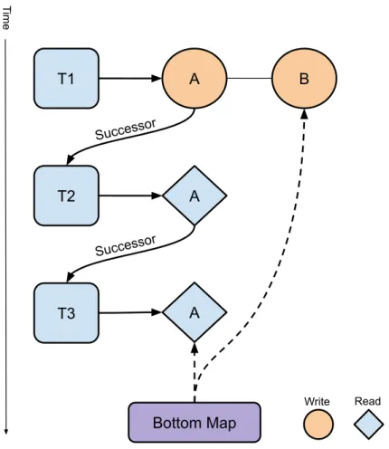
10.1 Sample code of a simple write-then-read program . . . 40
10.2 Dependency graph of a simple write-then-read program . . . 41
10.3 Sample code of a simple program with task nesting . . . 42
10.4 Dependency graph of a simple program with task nesting . . . 43
10.5 Double-check mechanism with locking to prevent race conditions. . . . 44
10.6 DataAccess structure and atomic top bit implementation. . . 45
11.1 Allocation of the TaskDataAccesses struct before optimization. . . 47
11.2 Task creation API with proposed change to pass access number. . . 48
11.3 Allocation of the TaskDataAccesses struct after optimization. . . 49
11.4 Code snippet of thenanos6 create task function showing adaptive mem-ory allocation. . . 49
11.7 BottomMapEntry layout after implementing reductions. . . 51
11.8 DataAccess layout after implementing reductions. . . 52
11.6 High-level illustration of a task reduction . . . 53
12.1 Scalability and speedup plots of the Multisaxpy benchmark with a prob-lem size of 1G eprob-lements . . . 56
12.2 Scalability and speedup plots of the Dot Product benchmark without using reduction and a problem size of 512M elements . . . 57
12.3 Scalability and speedup plots of the Dot Product benchmark using re-duction and a problem size of 512M elements . . . 57
12.4 Scalability and speedup plots of the Cholesky benchmark with a problem size of 32*32K elements . . . 58
12.5 Scalability and speedup plots of the Heat Equation benchmark with a problem size of 16*16K elements . . . 59
12.6 Scalability and speedup plots of the Matrix Multiply benchmark with a problem size of 2*8*2K elements . . . 60
12.7 Scalability and speedup plots of the N-body benchmark with a problem size of 16K particles and 10 time steps . . . 61
12.8 Peak memory usage and total allocations of the N-body benchmark with a problem size of 16K particles and 10 time steps . . . 62
12.9 Scalability and speedup plots of the HPCCG benchmark with a problem size of 250 nodes/processor . . . 63
List of Tables
5.1 Estimated time in hours required to do each of the tasks. . . 16
5.2 Prerequisites for each task. . . 17
6.1 Cost of human resources. . . 22
6.2 Cost of software resources. . . 23
6.3 Cost of hardware resources. . . 23
6.4 Indirect costs. . . 24
6.5 Final budget. . . 25
7.1 Sustainability matrix and scores. . . 26
12.1 Software versions present on the CTE-KNL supercomputer during the final evaluation . . . 55
1
|
Introduction
Parallel programming is a difficult task. The process of transforming a sequential pro-gram into a parallel one is not straightforward and, even then, achieving the maximum degree parallelism and scalability for a given problem (and thus, the maximum per-formance) is even more difficult. As it poses such a challenge, several programming models exist with the goal of making this task easier to tackle.
Those programming models often offer different levels of abstraction. In the lowest abstraction level we find the pthreads model, part of the POSIX.1 Standard [1], and in the highest we find the domain-specific languages or DSLs. In between, there are other models which aim to provide a balance between ease of use, generality and performance, such as Cilk, Intel TBB, OpenMP, and the OmpSs family [2–5].
1.1
Motivation
This work focuses on the OmpSs-2 programming model [5], developed by the Barcelona Supercomputing Center (BSC). This model features a data-flow execution schema, in which the programmer adapts the software by using compiler annotations to split the code into tasks and indicating for each task on which input and output data structures it operates. Then the runtime system, based on the user provided annotations, executes the program in parallel if it can guarantee that the result would be equivalent to a sequential execution of the same program.
The data-flow execution model will ensure that the final result is correct by using the information provided by the programmer about the tasks to schedule them in such a way that doesn’t break the constraints of a sequential model, while providing as much parallelism as possible. This is done through the concept of data dependencies inside the OmpSs-2 runtime, called Nanos6. The runtime calculates the dependency graph through the inputs and outputs declared by each task, and allows parallel execution of all the tasks that can be scheduled without breaking the sequential model.
The section of the Nanos6 runtime that calculates the dependencies and allows or holds the execution of the different tasks is the dependency subsystem, and it is one of the most important components of the runtime, as it is responsible for the parallel execution of the tasks and must ensure the equivalency of that execution to a sequential one, and thus forms the core of the data-flow execution model.
However, the dependency subsystem already implemented in the Nanos6 runtime is very complex, because it has to support all the features provided by the OmpSs-2 specification for the task construct, which are a lot since it is the main part of the model, and some programs do not need such a complete set of features as they have simpler data models.
This work focuses on the implementation of a simpler dependency subsystem for the Nanos6 runtime with less features than the existing one, but achieving better perfor-mance/scalability for certain task granularities. Additionally, the users of the runtime will be able to select which implementation of the dependency subsystem they want to use for different executions of their programs without the need to recompile all the libraries nor their programs.
1.2
Actors
The following roles will be needed during the development of this project.
• Developer: Responsible for writing the implementation that has been designed
and agreed by both the developer and the director of the project. The Developer will also be in charge of writing the final thesis, designing the project plan, code analysis, coding, project management, research and documentation. In this case, it’s the student doing the college thesis.
• Support Staff: Responsible of helping the developer carry out all tasks in the
project’s scope. In this case, the staff is the BSC’s Programming Models team which works or has worked with the runtime and their experience will be of high value to the developer.
• Directors: They will supervise the developer, mainly through face-to-face
meet-ings and emails. They will also have a strong influence in the technical decisions made during the implementation.
• Users and beneficiaries: The beneficiaries of this project will be the users of the
Nanos6 runtime, which will be staff of the BSC, MareNostrum users that use OmpSs-2 and anyone in the world that chooses to download the GPL-licensed version of the runtime [6]. Also, this code may serve as a future reference for newer versions or different parallel programming models, as it is open-sourced.
2
|
State of the art
This chapter provides context for the project by introducing related work through history and detailing the current state of the matter.
2.1
Parallel programming models
Parallel programming was born with the first supercomputers, that solved the need for more performance by having several CPUs, which would allow to speed up software as described by Amdahl’s Law [7]. As such, High Performance Computing was the main motivation behind the first parallel programming languages and models, and it allowed for asynchronous programming in single-core CPU machines as well.
During the 1990s, several models were created, but one of the first ones to gain rele-vance was MIT’s Cilk [2], based on the concept ofWork Stealing [8]. Cilk was the first runtime for parallel programming that guaranteed near-optimal performance, strict correctness and predictable runtime for writing parallel software. It was based on a thread graph model where when one of the threads ran out of work, it would steal a task from another. It ran on the supercomputers of the era and, most importantly, it served as inspiration for future shared-memory based parallel models.
Shortly after some other standards such as OpenMP [9] and Intel Threading Building Blocks [3] appeared, based on the same shared-memory communication mechanism and the idea of annotating a sequential program to exploit parallelism while producing the same results as the sequential version.
2.1.1
OpenMP
OpenMP is a case worth studying, because it has become a standard in writing parallel programs. It was based on afork-join execution model [4] that allows the programmer to define regions in the program that will be executed in parallel, and everything can be done by annotating the source code (in the case of C, with #pragma directives). The idea to annotate a sequential program, that could still be valid without annotations, and turn it into a parallel one, has been one of its main selling points.
Later, with the introduction of thetask construct and dependencies, it also supported a different data-flow execution model, where no explicit synchronization mechanisms were needed.
There has been, however, some criticism during the years, specially regarding the missing support for tasks at the start, and the non-asynchronous parallelism focus, that have been enough to cause the creation of other programming models during the years.
That being said, major compiler support for OpenMP [10] is outstanding, including: GCC, Clang, Intel, IBM and more, so it is very established in the industry.
2.1.2
OmpSs and OmpSs-2
OmpSs, its successor OmpSs-2, and the StarSs model family in general, have been some of the fore-runner programming models to the OpenMP standard [5]. Their main goal is to be a testing ground for innovations and new concepts in the parallel programming research. Concepts introduced first on this programming models have later been adopted by the OpenMP standard, as explained in Subsection 2.1.3. The StarSs family was created and is still being developed at the Barcelona Supercom-puting Center. They feature only a data-flow execution model, simplifying over the OpenMP model but inheriting the concept of transforming programs through compiler annotation. Tasks are the main units of work in OmpSs and OmpSs-2, and they are ordered into execution to guarantee sequential equivalency thanks to the input and output data specified by the programmer.
Another of the main focuses of OpenSs-2 is the ability to offload work to different architectures and devices, transferring execution of tasks to GPUs and FPGAs in a way that is transparent for the programmer, becoming effectively a heterogeneous model.
2.1.3
Influence in OpenMP
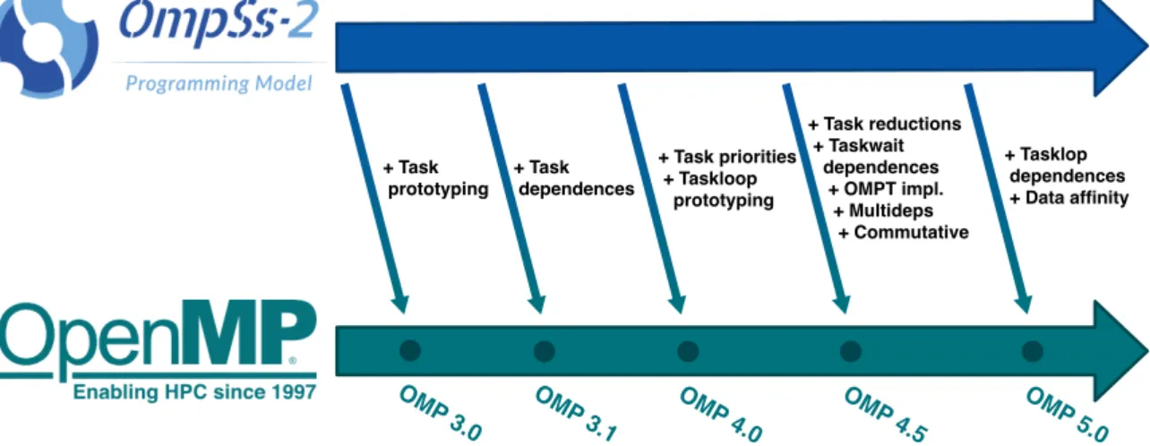
The OpenMP standard is alive and has added during its lifetime many features that have been implemented before on other programming models. Specifically, many of the features that have been proposed and developed at the Barcelona Supercomputing Center for its OmpSs models have been later added to the standard, to see more mainstream use. Figure 2.1 shows some of the features that have been added to some versions of the OpenMP standard after being implemented first on OmpSs or its predecessors.
OMP 3.0 OMP 3.1 OMP 4.0 OMP 4.5 OMP 5.0 + Task prototyping + Task dependences + Task priorities + Taskloop prototyping + Task reductions + Taskwait dependences + OMPT impl. + Multideps + Commutative + Tasklop dependences + Data affinity
Fig. 2.1: OmpSs-2 features that have influenced the OpenMP standard.
The work done at the BSC on the OmpSs-2 model and its runtime, Nanos6, can be understood as experimentation on features that may be later incorporated to the standard if they prove to be able to be efficiently implemented and provide measurable advantages.
2.2
Data dependencies
Parallel programming models often require the programmer to specify what data is going to be accessed during a task, and what type of access will be done (read, write, both...). This is so a dependency graph between the tasks can be calculated, and the runtime can ensure the final result will be the same than a sequential program. If the same data is used in two sibling tasks, those two tasks have a data dependency between them.
In particular, we can distinguish three types of data dependencies that can cause race conditions [11]:
1. True dependence (RAW). Read after write. Happens when a task T1 outputs
data that is going to be read by a task T2.
2. Antidependence (WAR). Write after read. Happens when a task T1 reads data
that is going to be overwritten by a task T2.
3. Output dependence (WAW). Write after write. Happens when a task T1 writes
data that is going to be overwritten by a task T2.
Altering the order of operations in any of the above cases can cause a data race and hence an incorrect result in the execution of a program. Thus, any parallel program-ming model that does data-flow execution needs to be able to know when a RAW, WAR or WAW dependency can happen, and ensure correct synchronization to prevent races.
OpenMP supports a simple data dependency model through itstask construct [4]. It allows for discrete dependencies between tasks at the same level of nesting, and the runtime will ensure correct execution constraints for those dependencies, by calculating a dependency graph and identifying potential data race conditions.
Other models support more complex dependencies, which allow the runtime to take more informed decisions about the task ordering, because they allow the programmer to specify more precisely the nature of those dependencies in the code. OmpSs-2 is one of those models [5], as data dependencies are the main mechanism to order task execution.
2.3
OmpSs-2 dependency model
OmpSs-2 extends the discrete dependency model of OpenMP to allow more fine-grained control through theweakin andweakout constructs [12]. In OpenMP’s model, if task nesting is used, two tasks with different parents cannot be directly linked through a data dependency, because they will only work with tasks on the same level. Instead, the programmer is forced to define the dependencies between the parent tasks, even if it is really the child tasks having the dependency.
This can cause a performance penalty, because at some point there may be tasks that could have started the execution and are waiting due to the dependencies not being fine-grained enough.
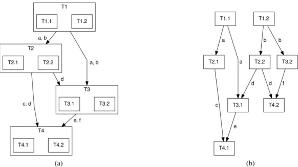
In Figure 2.2 it is clear that Task 2.1 could be executed before Task 1.2 finishes, because they have no real dependencies. This would result in a performance penalty in a model without theweakin andweakout clause. These two clauses are used between the parent tasks (T1 and T2, for instance) and tell the runtime that those two tasks have a dependency that is not caused directly by them, but by one of their child tasks, that will make them explicit with the in and out constructs. With this, the runtime has enough information to achieve a better performance, potentially.
In fact, even parent tasks that are dependent through weakdepend clauses can be executed concurrently, because the runtime has the knowledge that as long as their child tasks are not executed, the result will be correct because the parents have no real dependency.
Fig. 2.2: Data dependencies without and with the weakin/weakout constructs
Another particularity of the OmpSs-2 dependency model is that the user can specify dependencies for sections of memory (that do not need to be contiguous), not just discrete points, and thus the runtime can track the dependencies by regions and have more parallelism for some user cases. In figure 2.3 there are examples of the OmpSs-2 API for the different dependencies.
1 int main () {
2 int a[500];
3 int b[500];
4
5 // Discrete dependencies without weak constructs. 6 #pragma oss task in(a) out(b)
7 doSomething();
8 // Discrete dependencies with weak constructs. 9 #pragma oss task weakin(a) weakout(b)
10 doSomethingElse();
11 // Region dependencies
12 #pragma oss task in(a[0:499]) out(b[0:249])
13 anotherComputation();
14 }
Fig. 2.3: Examples of an OmpSs-2 annotated program
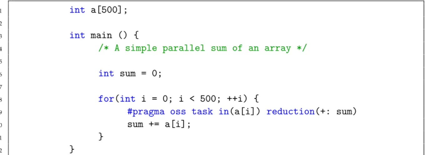
The OmpSs-2 spec also includes support for reductions in the task construct [5, 13], which allow the programs to combine or accumulate results obtained in different tasks
without the need for any explicit synchronization mechanism, such as atomics or barri-ers, increasing performance. The runtime supporsweakreductions as well, which enable reduction nesting. Reductions are seen by the runtime as just another type of data dependency, and they are registered as such through the API.
Figure 2.4 showcases a simple use of a task reduction to combine results of different tasks without the need to explicitly synchronize access to data.
1 int a[500];
2
3 int main () {
4 /* A simple parallel sum of an array */ 5
6 int sum = 0;
7
8 for(int i = 0; i < 500; ++i) {
9 #pragma oss task in(a[i]) reduction(+: sum)
10 sum += a[i];
11 }
12 }
Fig. 2.4: Example of OmpSs-2 reductions
A fully functional implementation of the OmpSs-2 spec for data dependencies already exists, but because of the great amount of features supported, specially memory re-gion dependencies, that implementation has a very high degree of complexity and the overhead introduced might have a performance impact for some tasks with small gran-ularities. The objective of this thesis is to develop a new implementation with less features that will have better performance for some applications.
3
|
Scope
3.1
Goal
The main goal of this project is to design and write a correct and efficient implemen-tation of as much of the Nanos6 dependency subsystem as possible, applying parallel techniques, algorithms and architecture-aware programming that have been learned during the course of the student’s Informatics Engineering degree.
3.2
Requirements
• Design and code a correct implementation of the Nanos6 dependency subsystem. • Adapt the code to the standards and style of the Nanos6 project.
• Test and verify the correctness of the implementation.
• Achieve better performance than older implementations in as much cases as possible.
• Implement the maximum of dependency features without compromising that performance.
• Study and evaluate the final result and suggest future work with the knowledge gathered during the project.
3.3
Scope
At the beginning of the project, existing implementations will be analyzed by the developer to gain knowledge about the runtime and understand what and how needs to be changed, to discuss with the directors the nature of the changes to the runtime. During this phase, as much tests as possible will be written, to stress the runtime in different ways, and existing benchmarks will be prepared to be ran by the developer as well. This has two goals: to understand the use of the programming model from a
user point of view and to use those tests further down the line to verify the correctness of the new implementation. Both tests that use only one feature and tests that use multiple features in conjunction will be coded.
Then, the second phase will be related to prepare the runtime to have two or more different dependency subsystem implementations at the same time, and the user being able to dynamically select one at run time. This is needed because the new implemen-tation might not be feature-complete enough to be used in all of the user cases, and thus it is not a drop-in replacement.
The next phase will be to design and code the new implementation, possibly based on earlier versions but with the goal of being as simple as possible to start with, allowing for more complex enhancements down the line. During this process, the tests mentioned earlier will be executed at each step to verify the progress and prevent regressions.
Finally, an evaluation will be carried out, with many different benchmarks and on different systems, to get a general understanding of how the new version performs and its limitation versus old implementations. At last, after the approval from the directors, the thesis will be written.
3.4
Risks
3.4.1
Deviation of the project plan
If the chosen design performs worse than expected, the project timeline or cost might change in order to accomplish the project goal.
Should this happen, the possibility of expanding the timeline would have to be ex-plored, but this scenario can be prevented by doing a good job in the planning stage.
3.4.2
Introducing bugs to the runtime
Bugs are an integral part of software development, and they are caused by human limitations. In this case, difficult to reproduce bugs could add complexity to the project and endanger the project plan.
Software correctness cannot be totally guaranteed, but most bugs can be detected early using established and proven development methods, such as Test Driven Development [14], to detect them as soon as they enter the code. This is further explained in Subsection 5.1.3
3.4.3
Compilation and test times
The full Nanos6 runtime takes several minutes to compile. Even if only one file has changed, linking time is not negligible, and even then running all the tests and stressing the runtime will take time out of actual development.
The development method can be adapted to the situation by trying to compile fewer libraries of the runtime and do other tasks during compilation, but time will be lost due to this risk specially when doing quick troubleshooting.
3.4.4
Result variance
As there are infinite use cases for the runtime, some programs might perform better than others, and achieve different speedups.
Tests cases and performance benchmarks will feature as much variety as possible to ensure most use cases are being evaluated, not just a few.
3.4.5
Debug difficulties
With parallel software with big degrees of concurrency and other complexities, dead-locks or race conditions can be difficult to reproduce, find and solve.
The developer will have to learn how to use debugging tools in those cases and write specific tests to trigger edge-case behavior.
4
|
Methodology
4.1
Time management
To use the time as efficiently as possible, tasks in this project will be short and incre-mental, having between them working versions of the software. This is similar to the SCRUM philosophy, but other concepts of that methodology will not be used because the project will not be done in a team environment. By doing it this way, withSprints
of one week or two, the planning can be changed on the go and that will provide a lot of flexibility with timing and planning [15].
4.2
Progress tracking
To keep track of the work that has been done, weekly (if possible) meetings will be held with the director, and the status updated online on OneNote.
For code tracking, on the other hand, the Git version control system will be used, in tandem with the GitLab online portal that is already used by the Programming Models group at the Barcelona Supercomputing Center, both to monitor progress and to exchange patches with other developers if needed.
4.3
Validation
Using a Test Driven Development approach, that is materialized because tests will be written before a single line of runtime code, will help correctness to be ensured during all steps of the project. That way, the implementation can also be defined as functionally complete when all the tests pass.
For performance, a set of benchmarks will be prepared to be run on different systems to gather speed-up statistics, and will also help finding bugs.
Finally, the final validation of the project will be done by the directors and the Barcelona Supercomputing Center.
4.4
Final result
The result expected for this project would be to get the code that has been developed merged into the master branch of OmpSs-2, reaching a release so that all the runtime users can access a better performance for smaller task granularities. The performance gain shall be quantified and proven through benchmark results in this thesis.
5
|
Project plan
This chapter describes the different tasks that define the project, the dependencies between them and the resources that will be used. All of this will be illustrated with a Gantt diagram in Section 5.6.
Finally, the possible setbacks that can be encountered during the project will be dis-cussed, in particular how they would affect the plan and the resources, and how they can be worked around if need be.
5.1
Tasks
The following subsections specify the different tasks that comprise the project.
5.1.1
Project management
This tasks encompasses all the content of theGesti´o de Projectes (GEP) subject, and its different deliverables. In total, five different tasks will be delivered totaling 75 hours of dedication, distributed the following way:
• Context and Scope: 24.5 hours • Project plan: 8.25 hours
• Economical plan and sustainability: 9.25 hours • Specialization module: 12.5 hours
• Oral presentation and final document: 18.25 hours
The tools Google Drive, Microsoft Office, Gantter, Google, Atenea and El Rac´o will be used during the course of the subject.
5.1.2
Runtime analysis
Before starting to write new code, it is very important to analyze the code that is already there, and what the rest of the system expects out of it. This will provide an understanding of what needs to change and help prevent bugs down the road caused by misunderstanding what the code really does.
This task will also encompass the time the developer will need to become familiar with the compiler, debugging tools and environment needed for the runtime.
The following tools will be used during this task: Git, GitLab, Visual Studio Code, Vim, CLion, Mercurium, GCC and Bash.
5.1.3
Correctness tests
As has been mentioned in earlier sections, tests will be created to ensure correctness. The tests will be small and totally independent programs that will use the OmpSs-2 tasks and dependencies, each one in a different way, to get as much coverage as possible. Each program will initialize the data, then do some parallel computation, and finally verify the result sequentially. High number of iterations, excessive task granularity and other techniques will be used in the tests to stress the runtime as much as possible. The tests will be easy to run as well, so they can be ran automatically each time the runtime is compiled to verify no bugs were introduced.
To create the tests C will be used as the programming language, the Mercurium
compiler and a code editor.
5.1.4
Initial implementation
Next, an initial implementation of the dependency subsystem will be designed and written, either from scratch or based on an already-existing one. The focus will be to keep it simple so optimizations and features can be introduced without a lot of development effort.
C++ will be used as the implementation language, compiled with the GCC (GNU Compiler Collection), and any of the code editors available.
5.1.5
Optimization
The optimization of the runtime consists on identifying the bottlenecks and address-ing them one by one. The developer will have to find the bottlenecks and come up with creative and simple ideas to solve them without introducing great amounts of complexity. The goal will be to enhance the initial implementation, both with new features and better performance.
C++ will be used as the implementation language, compiled with the GCC (GNU Compiler Collection), and any of the code editors available.
5.1.6
Evaluation
With the correctness tests, explained in 5.1.3, and benchmarks readily available at the BSC or sourced from elsewhere, the performance gains of the new dependency subsystem versus the original will be evaluated objectively.
The benchmarks may be run at some of the different supercomputers available at the BSC, and to make the task easier, an automatic build and run script will be created, to collect and save the execution times and results of the different benchmarks. The benchmarks implementation language may be C++ or C, they will be compiled with Mercurium and any scripts that need to be written will be done in either Bash
orPython.
5.1.7
Thesis writing
Finally, with all the research, knowledge and results gathered during the project, the final thesis will be written and future work may be proposed.
To write the thesis, LATEXwill be used, with Visual Studio Code as the editor,pdflatex as the compiler, and any web search engines, books or sources that are needed.
5.2
Timing
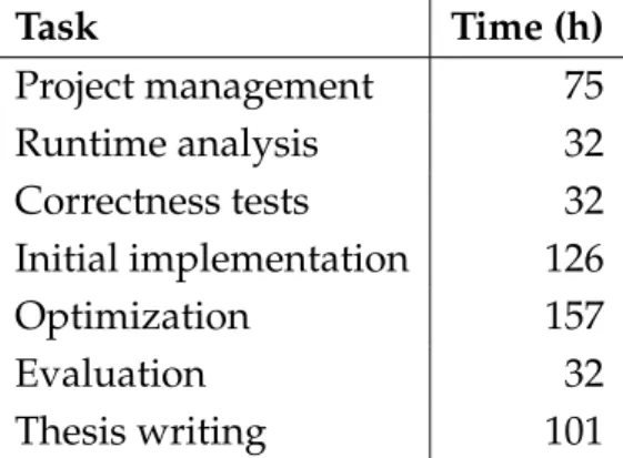
Table 5.1 shows the estimated time to do each of the tasks specified in section 5.1.
Task Time (h) Project management 75 Runtime analysis 32 Correctness tests 32 Initial implementation 126 Optimization 157 Evaluation 32 Thesis writing 101
5.3
Task dependencies
Some of the tasks that have been defined in 5.1 require other tasks to be completed before they can be started. Table 5.2 shows prerequisites for each task, if applicable.
Task Prerequisite
Project management
-Runtime analysis Project management Correctness tests Project management Initial implementation Runtime analysis
Correctness tests Optimization Initial implementation
Evaluation Optimization
Thesis writing Evaluation Table 5.2: Prerequisites for each task.
5.4
Resources
Different types of resources will be needed for this project, mainly human, hardware, and software.
5.4.1
Hardware
A laptop will be provided by the Barcelona Supercomputing Center, as well as a screen, for the purpose of this project. Also, the developer may work at home with a more-powerful home PC for any reason. Finally, more than one supercomputer may be used to check performance and correctness, but only the CTE-KNL supercomputer is specified here, as it will be the main resource used during the final evaluation task. For each system, CPU and memory available is specified, as well as any other notable features.
• BSC Laptop
– CPU: Intel® Core™ i7-5600U (2 cores, 4 threads, 2.6GHz)
– Memory: 16GB • Home PC
– Memory: 16GB
– GPU: NVIDIA GTX1060 • CTE-KNL Supercomputer:
– Login nodes: CTE-KNL has 1 login node with the following configuration. ∗ CPU: Intel ®Xeon™ E7-8850 (80 cores, 8 NUMA nodes)
∗ Memory: 2TB
∗ Interconnect: GPFS 10GBit/s (fiber)
– Compute nodes: CTE-KNL has 16 compute nodes with the following con-figuration.
∗ CPU: Intel ®Xeon Phi™ 7230 (64 cores, 256 threads, 1.30 GHz) ∗ Memory: 96GB of main memory (90 GB/s), 16 GB of high bandwidth
memory (480 GB/s) in cache mode
∗ Interconnect: 100 Gbit OmniPath interface, GPFS 1Gbit
5.4.2
Software
This project will use a wide variety of software for the different tasks, as well as many libraries and such required for the runtime to compile. For this reason, only the main software is specified in this section, but other programs and tools with no cost associated will be used during the project.
• KDE Neon 16.04: GNU/Linux distribution on the student’s Home PC.
• Manjaro Linux: GNU/Linux distribution on the BSC laptop. It was chosen because of its bleeding-edge versions of tools and compilers.
• Microsoft Windows 10: Used for the GEP subject.
• Git: Decentralized version control system, used for code and the final thesis writing.
• GitLab: Git repository management server, already used by the BSC.
• GDB: the GNU Project Debugger, used to find and troubleshoot bugs in the runtime.
• Mercurium: source-to-source compiler, used in the BSC, to transform OmpSs-2 annotated code into valid C/C++.
• GCC: the GNU Compiler Collection, both used to compile the nanos6 runtime and by back-end of the Mercurium compiler.
• Vim: Console-based text editor. • Visual Studio Code: Text editor.
• CLion: C/C++ Integrated Development Environment.
• LATEX: Computer typewriting system used to write the final thesis. • Microsoft Office: Office package used for the GEP subject.
• Gantter: Online service used to create Gantt diagrams and do general project management.
5.4.3
Human resources
As was explained more in depth in Section 1.2, this project will count with a director and co-director, support staff, and the main resource that will be the developer. In this case, the student doing his final thesis.
5.4.4
Spaces
The developer will work from a desk at the BSC, which will allow for direct contact with other runtime developers, and will make it easy to have weekly meetings with the project director.
5.5
Workarounds and action plan
In the hypothetical case of deviations to the project plan, the workaround would be different if it is just a setback in the normal development workflow, for example not finishing one of the tasks planned for a week of development, or a bigger setback that endangers the project plan.
In the event of a setback inside the normal development workflow, because of unex-pected complexity, bugs, personal problems, etc., the planning can be adapted because of the flexibility that our Agile development model and week to week planning give. As such, it could be rethought how to spend the remaining time and the requirements for the next development cycle can be changed.
In case of something major, that affected possibly the hole project, for instance bu-reaucracy problems or one task becoming much bigger than expected, time could be cut on the optimization and features included in the runtime, at the cost of less per-formance / functionality than expected, but that would be addressed in future work if need be. That way, further effects on the project plan would be prevented.
5.6
Gantt diagram
2018 2019
September October November December January February March April May June
Project management Context and Scope Project plan Economical plan Specialization module Final document Runtime analysis Correctness tests Initial implementation Optimization Evaluation Final thesis
5.7
Deviations
The Gantt diagram presented in Section 5.6 represents the final timeline of the project. On the initial plan, the student was due to start working at the BSC on October, but several bureaucratic issues caused this not to be possible. This was due to a change in the BSC policies for visitors, and it took a lot of time of coming and going between the University and the center. When all those issues were finally dealt with, it was possible to start working on the project in February.
Aside from that delay in the starting date, the rest of the project plan has been fairly respected. Although the exact count of hours spent in the project is difficult to calculate, the dates that were estimated for the start and end of the different tasks have been accurate and there was no rush at the end to finish the thesis in time.
6
|
Economic management
This chapter breaks down all the costs related to the project and how to tackle possible deviations in the budget.
6.1
Direct costs
Direct costs are derived directly from the project. In this case, it is the human re-sources, the hardware and the software needed.
6.1.1
Human resources
The cost of labor for a Informatics Engineering student is approximated using the minimum wage of a student cooperation contract for the UPC as reference. As such, a cost of 8€/h is assumed. The hours of the BSC support staff invested in the student are added up as well, which have been estimated in 16 hours at market price.
Resource Price (€/h) Amount (h) Total (€) Informatics Engineering student 8 555 4440
BSC Support staff 20 16 320
Total 4760
Table 6.1: Cost of human resources.
6.1.2
Software
The price of the software will be calculated estimating the useful life of the licenses to obtain a price per hour, that can then be factored in for each task.
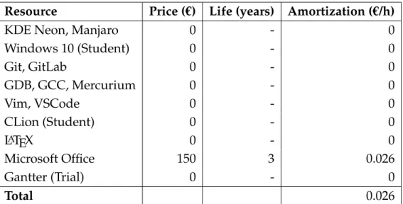
It is worth mentioning that most of the software in this project is free and open source, and thus it has no cost. This software will be omitted in the final budget for brevity, but is displayed here.
Resource Price (€) Life (years) Amortization (€/h)
KDE Neon, Manjaro 0 - 0
Windows 10 (Student) 0 - 0 Git, GitLab 0 - 0 GDB, GCC, Mercurium 0 - 0 Vim, VSCode 0 - 0 CLion (Student) 0 - 0 LATEX 0 - 0 Microsoft Office 150 3 0.026 Gantter (Trial) 0 - 0 Total 0.026
Table 6.2: Cost of software resources.
6.1.3
Hardware
There are two main hardware resources: the BSC laptop and the home PC. The amortization of the CTE-KNL supercomputer is calculated as well, but based only in one node (as only one at a time will be used during the project). However, its use is estimated at 12h/day, as the supercomputer has a lot of users inside and outside the BSC.
Resource Price (€) Life (years) Amortization (€/h)
Home PC 1200 4 0.16
BSC Laptop 2000 4 0.26
CTE-KNL (node) 10000 4 0.57
Total 0.99
Table 6.3: Cost of hardware resources.
6.2
Indirect costs
Indirect costs are caused by the project but not as a direct cause of its activities. In our project, the main indirect cost is the electricity used by the spaces and computers, and the home internet.
The assumptions made for this cost are that the home PC uses about 400 W, the BSC laptop about 50W and, based on the CTE-KNL CPU’s TDP of 215W, 500W for the full node accounting for cooling and other systems.
Resource Price Amount Total (€) Home PC Power 0.13847€/KWh 400Wh * 75 h 4.15 BSC Laptop Power 0.13847€/KWh 50Wh * 480 h 3.32 CTE-KNL Power 0.13847€/KWh 500Wh * 40 h 2.77 Internet 40€/month 5 months 200
Total 210.24
Table 6.4: Indirect costs.
6.3
Final budget
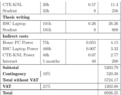
With the costs calculated earlier, and having an overall contingency of 10% and special budget for hiccups on the main tasks, the final project budget is presented in Table 6.5.
Resource Units Price (€/unit) Total (€) Project management Home PC 75h 0.16 12 Microsoft Office 75h 0.026 1.95 Student 75h 8 600 Runtime analysis BSC Laptop 32h 0.26 8.32 Student 32h 8 256 Correctness tests BSC Laptop 32h 0.26 8.32 Student 32h 8 256 Initial implementation BSC Laptop 126h 0.26 32.76 Student 126h 8 1008 Support Staff 8h 20 160 Setbacks 30h at 10% 0.8 24 Optimization BSC Laptop 157h 0.26 40.82 CTE-KNL 20h 0.57 11.4 Student 157h 8 1256 Support Staff 8h 20 160 Setbacks 30h at 20% 1.6 48 Evaluation
CTE-KNL 20h 0.57 11.4 Student 32h 8 256 Thesis writing BSC Laptop 101h 0.26 26.26 Student 101h 8 808 Indirect costs Home PC Power 75h 0.055 4.15 BSC Laptop Power 480h 0.007 3.32 CTE-KNL Power 40h 0.07 2.77 Internet 5 months 40 200 Subtotal 5203.79 Contingency 10% 520.38
Total without VAT 5724.17
VAT 21% 1202.08
Total 6926.25
Table 6.5: Final budget.
6.4
Risk management
Two different forms of risk contingencies are included in the final budget, just in case setbacks happen and threaten to deviate the costs.
First, in the two main development tasks, that have more changes of having hiccups because a lot of variables that affect those tasks cannot be accurately predicted, a 10% and 20% risk has been included, adding each risk a total of 30 hours of the student’s time in case it is needed.
Second, a 10% contingency item has been added to the final budget. The percentage is low because it is not foreseeable that any other material would need to be bought in any setback scenario, and thus the project would only need more time and the corresponding software/hardware amortization for the extra work. This will cover any other incidents that may happen and have not been accounted for in advance, and ensure the budget is respected regardless.
7
|
Sustainability
It is important to make an analytical reflection on the sustainability of the project to be able to justify its existence. This sustainability must not be just economical, but also social and environmental.
Table 7.1 represents the sustainability matrix of the project, where there is a brief summary of each of the elements and then a subjective score determined by the student. In the following sections on this chapter each of the elements of the matrix will be elaborated on. PPP Lifespan Risks Environmental 74KWh of partly renewable energy + commuting Reduction of emis-sions proportional to speedup Deviation from project plan or low speedup
8/10 10/10 6/10
Economic 6926.25€ Efficiency increase proportional to speedup
Deviation from project plan
10/10 8/10
Social Learning and ex-perience
Enhancement for users
None
10/10 10/10 10/10
Table 7.1: Sustainability matrix and scores.
7.1
Economic dimension
The cost of the project is not too high for being a five month endeavor, but under-standable as the main resource is a single student and almost no material is needed. In fact, the cost of the project to the BSC will be limited to just the space and a laptop, plus the hours of the director, as there is no internship involved.
per-supercomputer, and potentially many more systems around the world, as it is free software. Any improvement in performance will result in decreased software execution times, and time in a supercomputer is expensive. That way, it will cost less money to obtain the same results, because the software will be faster.
Aside from this, OmpSs has influenced the OpenMP spec heavily [5]. Many features that were first introduced in OmpSs have then been incorporated to the standard, and some of the reference implementations for those features were developed in the BSC. As such, the importance of having a good implementation is key, and it could decide if this features end up in OpenMP and benefit a much wider audience of users.
7.2
Social dimension
As an Informatics Engineering student, the main goal for the project is to learn. Being able to work side by side with the BSC and develop free software in a runtime used by other many developers, is a big learning opportunity and a great added value to the project. This is the main benefit the student will get from the college thesis.
The enhancement of a runtime will also affect directly to the quality of life of its users, now and in the future, as they will be able to write faster software retaining a lot of control over the data dependencies on their code. They will also gain confidence in the ability for Nanos6 to execute their code with good performance.
This new implementation also answers direct need of BSC staff, that need faster im-plementations with less features for certain cases, and simple code to be able to adapt to their needs easily.
7.3
Environmental dimension
All projects have an environmental impact, but the goal is to negate that impact with the benefits of the project during its lifespan. However, power used for the computers, and even fuel needed for commuting to and from the BSC, will create a footprint that cannot be ignored.
It will be a priority to reduce the environmental impact of the project as much as possible. This will include, among other things, using public transportation whenever possible for commuting. It is important to mention that the student’s home uses electricity sourced on its entirety from renewable energy, which will help reduce the CO2 emissions.
Once the modification to the runtime has been deployed, OmpSs-2 programs may have less execution time, and that is positive for the environment. A faster program is one that also, incidentally, uses less energy in order to execute. That will reduce the CO2 footprint of the programs.
Another effect will be towards supercomputer amortization. As there are always pro-grams running in theMareNostrum, the power bill is unlikely to be reduced, but if the software that runs on the supercomputer is faster, greater efficiency is achieved, more programs will be executed in the same amount of time. That is better for equipment amortization, not only economically, but environmentally as well.
8
|
Analyzing the runtime
and writing tests
This chapter covers the process of familiarizing with the current Nanos6 runtime and the coding of tests to check that different features related to the dependency subsystem behave correctly.
This starts all the way from the instrumentation and source to source compilation done by the Mercurium compiler, a high level overview of the OmpSs-2 runtime, reading the spec and user interfaces, and then writing valid C OmpSs-2 programs.
8.1
Compiling the runtime
The first step of this process will be to get a system ready to execute OmpSs-2 pro-grams. It will be assumed that the Mercurium compiler is already installed on the system, as it is not the focus of this thesis. The importance of understanding the runtime compilation process will become apparent in Chapter 9.
The Nanos6 runtime uses the GNU Build System [16], also known as Automake to generate the different pieces needed for compilation. This allows developers to cre-ate makefiles and configure scripts for a wide variety of UNIX-like operating systems without having to hand-write all of them.
There are two important files for this process: the configure.ac file, which defines configuration options that the user will be able to specify when compiling the runtime, and theMakefile.am file, which is a higher-level Makefile that can use the flags defined in the configure script. All the files a developer wants to include in the final library must be added to that file.
The current compilation script includes an option to include different dependency subsystem implementations in the final binary. As there have been several iterations of the OmpSs-2 spec [5], several options can be chosen. However, due to the fact that there was a default value to be chosen and then the rest of implementations weren’t even compiled, they were outdated to the point they couldn’t be built anymore. The rest of the compiling process is the standard for any UNIX software tarball. Running the configure script, compiling the source and installing.
8.2
Writing and compiling OmpSs-2 programs
The process to write and compile C programs that use OmpSs-2 is very similar to writing programs with OpenMP, but instead of using the GCC compiler, Mercurium
is used. This section will walk through that process with a simple program, which without any parallelization, is shown in Figure 8.1.
1 int main(int argc, char *argv[])
2 {
3 for(int i = 0; i < 1000000; ++i) {
4 doComputation();
5 }
6 return 0;
7 }
Fig. 8.1: Simple C sequential program
Assuming doComputation() is expensive, this program may take a long time to execute. For the purpose of this example, it is assumed that all the calls to doComputation() have no data dependencies between them. As such, this program is parallelizable, and it can be annotated with OmpSs-2 pragmas to achieve parallel execution [5]. Figure 8.2 shows the same program annotated with OmpSs-2.
1 int main(int argc, char *argv[])
2 {
3 for(int i = 0; i < 1000000; ++i) {
4 #pragma oss task
5 doComputation();
6 }
7 return 0;
8 }
Fig. 8.2: Simple C parallel program
If the program in Figure 8.2 is compiled with the Mercurium compiler, it will be modified to dynamically load the runtime upon execution, and then execute the do-Computation() calls in parallel. More information on the OmpSs-2 API is available in the spec [5].
8.3
Runtime architecture
The Nanos6 runtime is a complex system composed of different parts with a high level of integration and interconnection between them. As it has many components, and the developer is not familiar with many of them, only some are highlighted, and then the ones that are relevant for the project are explained in more detail.
• Scheduler: Distributes and assigns tasks (work units) between the different threads when they are ready to be executed. It will accept hints from other subsystems to decide what order the tasks are executed in.
• Instrumentation: Receives calls from all of the different systems signaling events and situations. Then, depending on the compile flags, it will use that information to print it, display it as a graph, pass it to other programs such as Extrae [17], or do nothing on the optimized version.
• Loader: Binary the annotated programs are linked with. Explained in detail in 8.3.1.
• Dependency subsystem: Keeps track of the data dependencies and decides what tasks are allowed to start execution. Explained in detail in 8.3.2
8.3.1
Loader
The loader is a small binary that is compiled with the Nanos6 runtime, and it is the one all annotated programs are linked against. Its main task is to then load the correct Nanos6 library depending on the environment variables the program has been executed with.
This is because the runtime has differentflavors. Those flavors are essentially compi-lations of the runtime done with different flags that enable or disable certain verbosity, debug features, optimizations, etc. In its current form it is used by the user through
NANOS6 environment variable. Depending on that variable a certain flavor will be dynamically linked, and this way the user can enable different instrumentations. Essentially, the loader is just a stub to link the real runtime, but it will link differ-ent flavors without having to recompile it. Some examples of the currdiffer-ently available runtime flavors are: verbose, debug, stats, stats-papi, profile, extrae and graph.
8.3.2
Dependency subsystem
The dependency subsystem is the one that will receive all the information regarding the task’s data accesses, and then decide if that task can start execution, or it can’t because it would violate the dependency model.
During the project no deep dive into the details of the current implementation was done, because it is of little value as it is going to change, and because it would probably influence the design of the new implementation. However, it is really important to understand the entry points to the system, both internally and externally, and what its responsibilities are.
To save its state, the dependency subsystem has a class calledTaskDataAccesses that is a member of the main Task class. There, any relevant data structures are created to store the dependencies of the current task, and it will be allocated and destroyed with the task.
To maintain the state, the system has a series of functions that it exposes, either to the rest of components or even to the annotated program. They will be called in a specific order for each task, and allow the implementation to do any relevant operations on the data to ensure the dependency model is respected. Those functions are briefly explained here, and are called in the following order:
1. nanos6 register * depinfo: The * is substituted by the type of access (for example
write or read), and this functions are exposed through the loader and called directly from the annotated program. One call will be made for each data access that task has declared.
2. DataAccessRegistration::registerTaskDataAccess: This function is called from in-side the earlier one for each invocation, but is internal.
3. DataAccessRegistration::registerTaskDataAccesses: Called from thenanos6 sub-mit task function, only once per task, when all the accesses have been registered. This is where the dependencies and order are calculated.
4. DataAccessRegistration::handleEnterTaskwait / DataAccessRegistration::handle-TaskExitTaskwait: Called when the tasks enters or exits a taskwait. Is is worth mentioning that implicit taskwaits (ones at the end of a task code block) also call this function.
5. DataAccessRegistration::unregisterTaskDataAccesses: Called when the data ac-cesses of the task have been finished and dependencies can be satisfied.
6. DataAccessRegistration::handleTaskRemoval: Called whenever a task is being deleted from memory because it is not needed anymore.
To communicate to the rest of the runtime the status of the dependencies of a task, two counters in theTask class are changed:
1. Task::increasePredecessors / Task::decreasePredecessors: Marks the unsatisfied dependencies a task is pending on. When it reaches 0, the task can be scheduled.
2. Task::increaseRemovalBlockingCount / Task::decreaseRemovalBlockingCount: Keeps track on how many subsystems depend on that task remaining in memory to work, and hence are blocking the deallocation of the task. When it reaches 0, the task is deleted.
It must be noted that in the Nanos6 runtime, it is assumed that if a subsystem decreases to zero one of the counters of the earlier list, it is that subsystem’s responsibility to either enqueue the task in the Scheduler or call the task destructor and deallocate it.
8.4
Writing correctness tests
With all the information obtained and after reading the OmpSs-2 Spec[5], the test writing phase can be started. They are written as simple self-contained C programs, that might or might not have a useful purpose, but that its correct execution can be checked easily in a sequential manner.
The coded tests check many different features of the dependency model but in iso-lation. To enumerate some of those features, there are discrete dependencies, task nesting, reduction, reduction nesting, weak tasks, totally overlapping regions, par-tially overlapping regions in different ways, etc. The main goal has been to cover as many cases as possible with the tests, to ensure that if a bug is introduced it breaks a test.
During all of the project, if a bug is found that doesn’t break a test, a broken test just for that bug is created. After it, it is fixed, and checked with the new test that it is not introduced ever again. This is commonly known as regression testing [18].
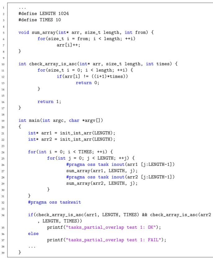
In Figure 8.3 the typical layout of a correctness test is displayed. It sets up the needed data, does some work, checks the result, and then displays wether it was a success or a failure. Then, with a shell script, all tests can be ran and regressions are easily spotted. This specific test focuses on partially overlapping memory regions.
1 ...
2 #define LENGTH 1024
3 #define TIMES 10
4
5 void sum_array(int* arr, size_t length, int from) {
6 for(size_t i = from; i < length; ++i)
7 arr[i]++;
8 }
9
10 int check_array_is_asc(int* arr, size_t length, int times) { 11 for(size_t i = 0; i < length; ++i) {
12 if(arr[i] != ((i+1)*times)) 13 return 0; 14 } 15 16 return 1; 17 } 18
19 int main(int argc, char *argv[])
20 {
21 int* arr1 = init_int_arr(LENGTH);
22 int* arr2 = init_int_arr(LENGTH);
23
24 for(int i = 0; i < TIMES; ++i) {
25 for(int j = 0; j < LENGTH; ++j) {
26 #pragma oss task inout(arr1 [j:LENGTH-1])
27 sum_array(arr1, LENGTH, j);
28 #pragma oss task inout(arr2 [j:LENGTH-1])
29 sum_array(arr2, LENGTH, j);
30 }
31 }
32 #pragma oss taskwait
33
34 if(check_array_is_asc(arr1, LENGTH, TIMES) && check_array_is_asc(arr2
, LENGTH, TIMES))
35 printf("tasks_partial_overlap test 1: OK");
36 else
37 printf("tasks_partial_overlap test 1: FAIL");
38 ...
39 }
Fig. 8.3: Example of a correctness test with tasks depending on memory regions with partial overlap
9
|
Adapting the runtime
for different implementations
This chapter explains how the runtime has been adapted, through a method of condi-tional compilation, to house two different implementations of the dependency subsys-tem that the user can switch without having to recompile.
The main purpose of this task is to be able to have both (original and new) versions of the dependency subsystem at the same time, as the next version may not have all the features the OmpSs-2 spec [5] requires, exchanged for performance in applications with low task granularity.
Please note, from this point onward, the original implementation will be referred as
linear-regions-fragmented, which is its internal name, and the new implementation as
discrete-simple.
9.1
Designing the mechanism
In the initial brainstorming phase, it had to be decided how to switch versions, and decide what technique was going to be used.
The first idea was to adapt the linear-regions-fragmented version to use the C++ version of an interface (an abstract class), that all the future versions could inherit from. That way versions can be switched at execution time, by having every current call to the dependency subsystem go through an implementation-agnostic interface. That idea, however, had several issues that made it unsuitable. First, the time invest-ment required to adapt the runtime in such a way was too much, as the Instruinvest-mentation subsystem relied on a lot of internal details of the linear-regions-fragmented version that could be easily mocked by other versions but was too time-consuming to abstract through interfaces.
The second issue, and the biggest one, was that all the data structures for the sub-system, housed in theTaskDataAccesses class, were allocated with the main task, and thus the size of those structures had to be known on compilation time. While decou-pling them to be allocated on a separate call would be possible, memory allocation is
very expensive and all the references to that structure across the whole runtime would have to be changed as well.
Another idea was to use a similar conditional compilation method that was already used for the different Nanos6 flavors and has been explained in Section 8.3.1. That way, the existing loader is repurposed to switch dependency implementations depending on environment variables, and this idea has none of the issues of the first one, because the two versions would be compiled to different libraries.
The conditional compilation method was not free of drawbacks, though. By having to compile all the different Nanos6 flavors as well with each implementation, the number of binaries generated and the already long compilation time is doubled. That, however, was acknowledged as an acceptable trade-off and thus this approach was chosen.
9.2
Implementing conditional compilation
In Section 8.1 it was explained what tools were used to compile the runtime, and the relevant files. To get all the flavors to compile with both implementations, the
configure.ac file was modified to provide switches to compile or omit each version. That way, if a user or developer is only interested in using one of the versions but not the other, they can be excluded from compilation, resulting in fewer binaries and lower compilation times.
The most important part, however, was to change theMakefile.am file and add defini-tions to build all the libraries twice, one for each version. That was done while trying to make it as easy as possible to add even more dependency implementations in the future, but the Automake tool has some limitations on its ability to define macros to be that portable (it doesn’t even have loops, for example).
After the adaptations both versions could compile at the same time, but adapting the Nanos6 loader was still necessary.
9.3
Modifying the loader
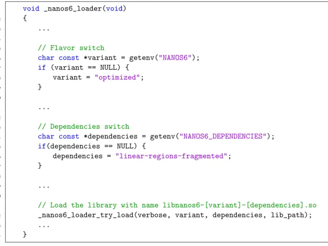
The Nanos6 loader, explained in Subsection 8.3.1, allows the dynamic linking of dif-ferent flavors by switching on environment variables. To be able to select the depen-dencies as well, a new environment variable NANOS6 DEPENDENCIES was added, with two possible values: linear-regions-fragmented and discrete-simple. Depending on that variable, the correct library will be linked to the annotated executable. For that, the existing loader, which already had support for different flavors, was modified by adding the dependency implementation name to the loaded library as well, and if no environment variable was set, defaulting to the feature-complete linear-regions-fragmented, so the user had a spec-compliant library if nothing was specified.
1 void _nanos6_loader(void)
2 {
3 ...
4
5 // Flavor switch
6 char const *variant = getenv("NANOS6");
7 if (variant == NULL) { 8 variant = "optimized"; 9 } 10 11 ... 12 13 // Dependencies switch
14 char const *dependencies = getenv("NANOS6_DEPENDENCIES");
15 if(dependencies == NULL) { 16 dependencies = "linear-regions-fragmented"; 17 } 18 19 ... 20
21 // Load the library with name libnanos6-[variant]-[dependencies].so 22 _nanos6_loader_try_load(verbose, variant, dependencies, lib_path);
23 ...
24 }
10
|
Initial implementation
This chapter covers the base design and code of the discrete-simple implementation. This was built based on another simple implementation that was developed earlier just to cover the needs of one particular use case. As the base code was adopted to cut down on development time, but does not represent the final design, details about it will be omitted.
10.1
Initial design
The basic idea of the implementation is that each task will have only two basic struc-tures to keep its dependencies:
• A Bottom map, which will have entries pointing to the last access to a certain memory address. That way, when registering its dependencies, a child task can go to its parent’s bottom map and determine if any of its siblings are accessing to the same memory addresses, and stablish a dependency relationship. The key of the map is the address. Inside one node of the bottom map, the following data is stored:
– The last access that has been registered to that address.
– A boolean indicating if that last access is satisfied.
• Anarray of accesses, that represent all the declared depend clauses of the current task. The actual addresses are stored in another array with the same indexes, to prevent long searches due to cache misses. For each memory access, the following information is:
– The access type, being for now either read, write, or readwrite.
– The successor task, which is the next sibling task that has registered an access to that address.
– An boolean indicating if the access is the top of a chain of read accesses.