13
Numerous mathematical-programming applications, including many introduced in previous chapters, are cast naturally as linear programs. Linear programming assumptions or approximations may also lead to appropriate problem representations over the range of decision variables being considered. At other times, though, nonlinearities in the form of either nonlinear objectivefunctions or nonlinear constraints are crucial for representing an application properly as a mathematical program. This chapter provides an initial step toward coping with such nonlinearities, first by introducing several characteristics of nonlinear programs and then by treating problems that can be solved using simplex-like pivoting procedures. As a consequence, the techniques to be discussed are primarily algebra-based. The final two sections comment on some techniques that do not involve pivoting.
As our discussion of nonlinear programming unfolds, the reader is urged to reflect upon the linear-programming theory that we have developed previously, contrasting the two theories to understand why the nonlinear problems are intrinsically more difficult to solve. At the same time, we should try to understand the similarities between the two theories, particularly since the nonlinear results often are motivated by, and are direct extensions of, their linear analogs. The similarities will be particularly visible for the material of this chapter where simplex-like techniques predominate.
13.1 NONLINEAR PROGRAMMING PROBLEMS
A general optimization problem is to select n decision variables x1,x2, . . . ,xn from a given feasible region
in such a way as to optimize (minimize or maximize) a given objective function
f(x1,x2, . . . ,xn)
of the decision variables. The problem is called a nonlinear programming problem (NLP) if the objective function is nonlinear and/or thefeasible region is determined by nonlinear constraints. Thus, in maximization form, the general nonlinear program is stated as:
Maximize f(x1,x2, . . . ,xn), subject to:
g1(x1,x2, . . . ,xn) ≤ b1,
... ...
gm(x1,x2, . . . ,xn) ≤ bm,
where each of the constraint functions g1through gm is given. A special case is the linear program that has
been treated previously. The obvious association for this case is
f(x1,x2, . . . ,xn)= n X j=1 cjxj, 410
13.1 Nonlinear Programming Problems 411 and gi(x1,x2, . . . ,xn)= n X j=1 ai jxj (i =1,2, . . . ,m).
Note that nonnegativity restrictions on variables can be included simply by appending the additional con-straints:
gm+i(x1,x2, . . . ,xn)= −xi ≤0 (i =1,2, . . . ,n).
Sometimes these constraints will be treated explicitly, just like any other problem constraints. At other times, it will be convenient to consider them implicitly in the same way that nonnegativity constraints are handled implicitly in the simplex method.
For notational convenience, we usually let x denote the vector of n decision variables x1,x2, . . . ,xn —
that is, x =(x1,x2, . . . ,xn)— and write the problem more concisely as
Maximize f(x),
subject to:
gi(x)≤bi (i =1,2, . . . ,m).
As in linear programming, we are not restricted to this formulation. To minimize f(x), we can of course maximize−f(x). Equality constraints h(x)=b can be written as two inequality constraints h(x)≤b and −h(x) ≤ −b. In addition, if we introduce a slack variable, each inequality constraint is transformed to an
equality constraint. Thus sometimes we will consider an alternative equality form: Maximize f(x),
subject to:
hi(x)=bi (i = 1,2, . . . ,m) xj ≥0 (j = 1,2, . . . ,n).
Usually the problem context suggests either an equality or inequality formulation (or a formulation with both types of constraints), and we will not wish to force the problem into either form.
The following three simplified examples illustrate how nonlinear programs can arise in practice.
Portfolio Selection An investor has $5000 and two potential investments. Let xj for j = 1 and j = 2
denote his allocation to investment j in thousands of dollars. From historical data, investments 1 and 2 have an expected annual return of 20 and 16 percent, respectively. Also, the total risk involved with investments 1 and 2, as measured by the variance of total return, is given by 2x12+x2
2+(x1+x2)
2, so that risk increases with total investment and with the amount of each individual investment. The investor would like to maximize his expected return and at the same time minimize his risk. Clearly, both of these objectives cannot, in general, be satisfied simultaneously. There are several possible approaches. For example, he can minimize risk subject to a constraint imposing a lower bound on expected return. Alternatively, expected return and risk can be combined in an objective function, to give the model:
Maximize f(x)=20x1+16x2−θ[2x12+x22+(x1+x2)2],
subject to:
g1(x) = x1+x2 ≤5,
x1 ≥ 0, x2 ≥0, (that is, g2(x)= −x1, g3(x)= −x2).
The nonnegative constantθ reflects his tradeoff between risk and return. Ifθ = 0, the model is a linear
program, and he will invest completely in the investment with greatest expected return. For very largeθ, the objective contribution due to expected return becomes negligible and he is essentially minimizing his risk.
Water Resources Planning In regional water planning, sources emitting pollutants might be required to remove waste from the water system. Let xj be the pounds of Biological Oxygen Demand (an often-used
measure of pollution) to be removed at source j .
One model might be to minimize total costs to the region to meet specified pollution standards:
Minimize n X j=1 fj(xj), subject to: n X j=1 ai jxj ≥bi (i=1,2, . . . ,m) 0≤xj ≤uj (j =1,2, . . . ,n), where
fj(xj)= Cost of removing xj pounds of Biological Oxygen Demand at
source j ,
bi = Minimum desired improvement in water quality at point i in the
system,
ai j = Quality response, at point i in the water system, caused by removing
one pound of Biological Oxygen Demand at source j ,
uj = Maximum pounds of Biological Oxygen Demand that can be
removed at source j .
Constrained Regression A university wishes to assess the job placements of its graduates. For simplicity, it assumes that each graduate accepts either a government, industrial, or academic position. Let
Nj =Number of graduates in year j (j =1,2, . . . ,n),
and let Gj,Ij,and Aj denote the number entering government, industry, and academia, respectively, in year j(Gj +Ij +Aj = Nj).
One model being considered assumes that a given fraction of the student population joins each job category each year. If these fractions are denoted asλ1, λ2, andλ3, then the predicted number entering the job categories in year j is given by the expressions
ˆ Gj = λ1Nj, ˆ Ij = λ2Nj, ˆ Aj = λ3Nj.
A reasonable performance measure of the model’s validity might be the difference between the actual number of graduates Gj, Ij, and Aj entering the three job categories and the predicted numbersGˆ j, Iˆj, and Aˆj, as
in the least-squares estimate: Minimize
n X
j=1
[(Gj − ˆGj)2+(Ij − ˆIj)2+(Aj − ˆAj)2],
subject to the constraint that all graduates are employed in one of the professions. In terms of the fractions entering each profession, the model can be written as:
Minimize
n X
j=1
13.2 Local vs. Global optimum 413
subject to:
λ1 + λ2+λ3=1,
λ1 ≥ 0, λ2≥0, λ3 ≥0. This is a nonlinear program in three variablesλ1,λ2, andλ3.
There are alternative ways to approach this problem. For example, the objective function can be changed to: Minimize n X j=1 h Gj − ˆGj| + |Ij − ˆIj| + |Aj − ˆAj i .†
This formulation is appealing since the problem now can be transformed into a linear program. Exercise 28 (see also Exercise 20) from Chapter 1 illustrates this transformation.
The range of nonlinear-programming applications is practically unlimited. For example, it is usually simple to give a nonlinear extension to any linear program. Moreover, the constraint x = 0 or 1 can be modeled as x(1−x) =0 and the constraint x integer as sin(πx) =0. Consequently, in theory any application of
integer programming can be modeled as a nonlinear program. We should not be overly optimistic about these formulations, however; later we shall explain why nonlinear programming is not attractive for solving these problems.
13.2 LOCAL vs. GLOBAL OPTIMUM
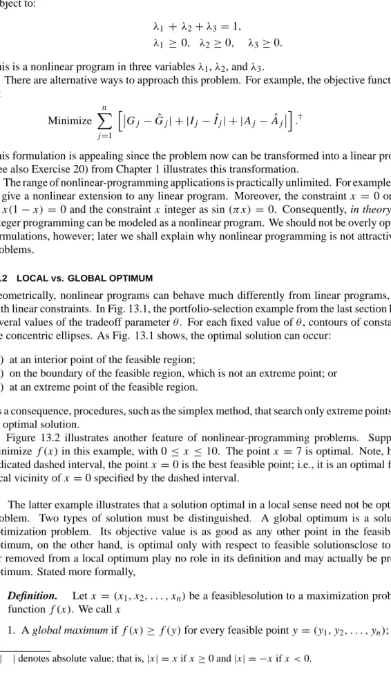
Geometrically, nonlinear programs can behave much differently from linear programs, even for problems with linear constraints. In Fig. 13.1, the portfolio-selection example from the last section has been plotted for several values of the tradeoff parameterθ. For each fixed value ofθ, contours of constant objective values are concentric ellipses. As Fig. 13.1 shows, the optimal solution can occur:
a) at an interior point of the feasible region;
b) on the boundary of the feasible region, which is not an extreme point; or c) at an extreme point of the feasible region.
As a consequence, procedures, such as the simplex method, that search only extreme points may not determine an optimal solution.
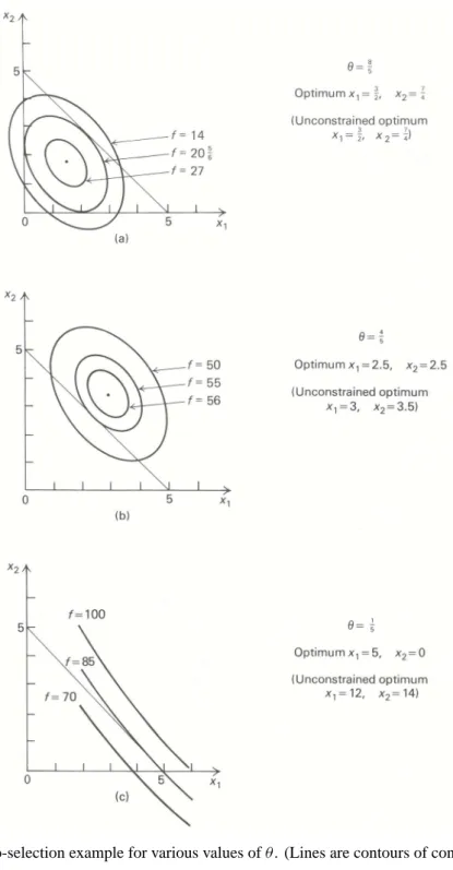
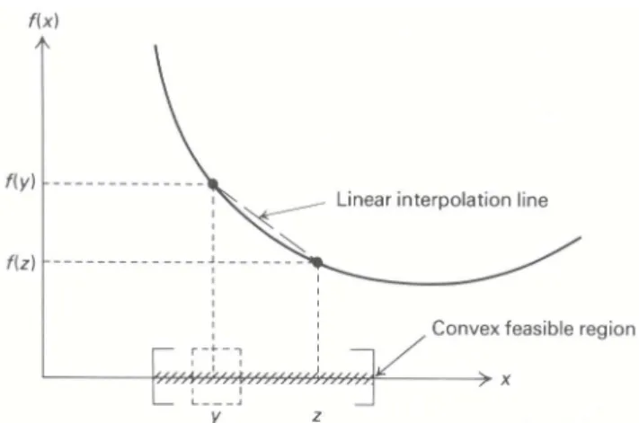
Figure 13.2 illustrates another feature of nonlinear-programming problems. Suppose that we are to minimize f(x)in this example, with 0≤ x ≤ 10. The point x =7 is optimal. Note, however, that in the indicated dashed interval, the point x =0 is the best feasible point; i.e., it is an optimal feasible point in the
local vicinity of x =0 specified by the dashed interval.
The latter example illustrates that a solution optimal in a local sense need not be optimal for the overall problem. Two types of solution must be distinguished. A global optimum is a solution to the overall optimization problem. Its objective value is as good as any other point in the feasible region. A local optimum, on the other hand, is optimal only with respect to feasible solutionsclose to that point. Points far removed from a local optimum play no role in its definition and may actually be preferred to the local optimum. Stated more formally,
Definition. Let x =(x1,x2, . . . ,xn)be a feasiblesolution to a maximization problem with objective
function f(x). We call x
1. A global maximum if f(x)≥ f(y)for every feasible point y =(y1,y2, . . . ,yn); †| |denotes absolute value; that is,|x| =x if x≥0 and|x| = −x if x<0.
13.3 Convex and Concave Functions 415
Figure 13.2 Local and global minima.
2. A local maximum if f(x)≥ f(y)for every feasible point y =(y1,y2, . . . ,yn)sufficiently close to x. That is, if there is a number >0 (possibly quite small) so that, whenever each variable yj is within of xj — that is, xj − ≤ yj ≤ xj +—and y is feasible, then f(x)≥ f(y).
Global and local minima are defined analogously. The definition of local maximum simply says that if we place an n-dimensional box (e.g., a cube in three dimensions) about x, whose side has length 2, then f(x)
is as small as f(y)for every feasible point y lying within the box. (Equivalently, we can use n-dimensional spheres in this definition.) For instance, if =1 in the above example, the one-dimensional box, or interval,
is pictured about the local minimum x =0 in Fig. 13.2.
The concept of a local maximum is extremely important. As we shall see, most general-purpose nonlinear-programming procedures are near-sighted and can do no better than determine local maxima. We should point out that, since every global maximum is also a local maximum, the overall optimization problem can be viewed as seeking the best local maxima.
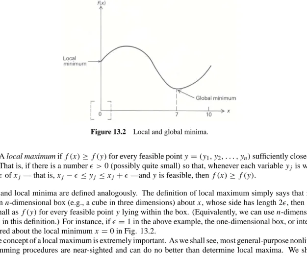
Under certain circumstances, local maxima and minima are known to be global. Whenever a function ‘‘curves upward’’ as in Fig. 13.3(a), a local minimum will be global. These functionsare called convex. Whenever a function ‘‘curves downward’’ as in Fig. 13.3(b) a local maximum will be a global maximum. These functions are called concave.† For this reason we usually wish to minimize convex functions and maximize concave functions. These observations are formalized below.
13.3 CONVEX AND CONCAVE FUNCTIONS
Because of both their pivotal role in model formulation and their convenient mathematical properties, certain functional forms predominate in mathematical programming. Linear functions are by far the most important. Next in importance are functions which are convex or concave. These functions are so central to the theory that we take some time here to introduce a few of their basic properties.
An essential assumption in a linear-programming model for profit maximization is constant returns to scale for each activity. This assumption implies that if the level of one activity doubles, then that activity’s profit contribution also doubles; if the first activity level changes from x1to 2x1, then profit increases proportionally from say $20 to $40 [i.e., from c1x1to c1(2x1)]. In many instances, it is realistic to assume constant returns to scale over the range of the data. At other times, though, due to economies of scale, profit might increase disproportionately, to say $45; or, due to diseconomies of scale (saturation effects), profit may be only $35. In the former case, marginal returns are increasing with the activity level, and we say that the profit function
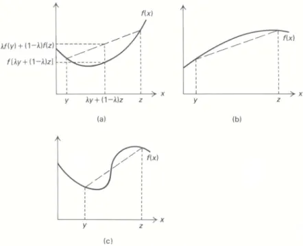
Figure 13.3 a) Convex function b) concave function (c) nonconvex, nonconcave function.
is convex (Fig. 13.3(a)). In the second case, marginal returns are decreasing with the activity level and we say that the profit function is concave (Fig.13.3(b)). Of course, marginal returns may increase over parts of the data range and decrease elsewhere, giving functions that are neither convex nor concave (Fig. 13.3(c)).
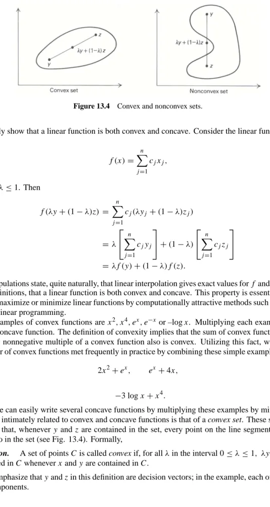
An alternative way to view a convex function is to note that linear interpolation overestimates its values. That is, for any points y and z, the line segment joining f(y)and f(z)lies above the function (see Fig. 13.3). More intuitively, convex functions are ‘‘bathtub like’’ and hold water. Algebraically,
Definition. A function f(x)is called convex if,for every y and z and every 0≤λ≤1,
f[λy+(1−λ)z] ≤λf(y)+(1−λ)f(z).
It is called strictly convex if, for every two distinct points y and z and every 0< λ <1,
f[λy+(1−λ)z]< λf(y)+(1−λ)f(z).
The lefthand side in this definition is the function evaluation on the line joining x and y; the righthand side is the linear interpolation. Strict convexity corresponds to profit functions whose marginal returns are strictly increasing.
Note that although we have pictured f above to be a function of one decision variable, this is not a restric-tion. If y = (y1,y2, . . . ,yn)and z =(z1,z2, . . . ,zn), we must interpretλy+(1−λ)z only as weighting the decision variables one at a time, i.e., as the decision vector (λy1+(1−λ)z1, . . . , λyn+(1−λ)zn).
Concave functions are simply the negative of convex functions. In this case, linear interpolation under-estimates the function. The definition above is altered by reversing the direction of the inequality. Strict concavity is defined analogously. Formally,
Definition. A function f(x)is called concave if,for every y and z and every 0≤λ≤1, f[λy+(1−λ)z] ≥λf(y)+(1−λ)f(z).
It is called strictly concave if, for every y and z and every 0< λ <1,
13.3 Convex and Concave Functions 417
Figure 13.4 Convex and nonconvex sets.
We can easily show that a linear function is both convex and concave. Consider the linear function:
f(x)= n X
j=1
cjxj,
and let 0≤λ≤1. Then
f(λy+(1−λ)z) = n X j=1 cj(λyj +(1−λ)zj) = λ n X j=1 cjyj +(1−λ) n X j=1 cjzj = λf(y)+(1−λ)f(z).
These manipulations state, quite naturally, that linear interpolation gives exact values for f and consequently, from the definitions, that a linear function is both convex and concave. This property is essential, permitting us to either maximize or minimize linear functions by computationally attractive methods such as the simplex method for linear programming.
Other examples of convex functions are x2,x4,ex,e−xor –log x. Multiplying each example by minus one gives aconcave function. The definition of convexity implies that the sum of convex functions is convex and that any nonnegative multiple of a convex function also is convex. Utilizing this fact, we can obtain a large number of convex functions met frequently in practice by combining these simple examples, giving, for instance,
2x2+ex, ex+4x,
or
−3 log x+x4.
Similarly, we can easily write several concave functions by multiplying these examples by minus one. A notion intimately related to convex and concave functions is that of a convex set. These sets are ‘‘fat,’’ in the sense that, whenever y and z are contained in the set, every point on the line segment joining these points is also in the set (see Fig. 13.4). Formally,
Definition. A set of points C is called convex if, for allλin the interval 0≤λ≤1, λy+(1−λ)z is
contained in C whenever x and y are contained in C.
Again we emphasize that y and z in this definition are decision vectors; in the example, each of these vectors has two components.
We have encountered convex sets frequently before, since the feasible region for a linear program is convex. In fact, the feasible region for a nonlinear program is convex if it is specified by less-than-or-equal-to equalities with convex functions. That is, if fi(x)for i =1,2, . . . ,m, are convex functions and if the points x =y and x =z satisfy the inequalities
fi(x)≤bi (i =1,2, . . . ,m),
then, for any 0≤λ≤1,λy+(1−λ)z is feasible also, since the inequalities fi(λy+(1−λ)z)≤λfi(y)+(1−λ)fi(z)≤ λbi +(1−λ)bi =bi
↑ ↑
Convexity Feasibility of y and z
hold for every constraint. Similarly, if the constraints are specified by greater-than-or-equal-to inequali-ties and the functions are concave, then the feasible region is convex. In sum, for convex feasible regions we want convex functions for less-than-or-equal-to constraints and concave functions for greater-than-or-equal-to constraints. Since linear functions are both convex and concave, they may be treated as equali-ties.
An elegant mathematical theory, which is beyond the scope of this chapter, has been developed for convex and concave functions and convex sets. Possibly the most important property for the purposes of nonlinear programming was previewed in the previous section. Under appropriate assumptions, a local optimumcan be shown to be a global optimum.
Local Minimum and Local Maximum Property
1. A local minimum maximum of a convex concave
function on a convex feasible region is also a
global minimum maximum . 2. A local minimum maximum of a strictly convex concave
function on a convex feasible region
is the unique global
minimum maximum
.
We can establish this property easily by reference to Fig. 13.5. The argument is for convex functions; the concave case is handled similarly. Suppose that y is a local minimum. If y is not a global minimum, then, by definition, there is a feasible point z with f(z) < f(y). But then if f is convex, the function must lie on or below the dashed linear interpolation line. Thus, in any box about y, there must be an x on the line segment joining y and z, with f(x) < f(y). Since the feasible region is convex, this x is feasible and we have contradicted the hypothesis that y is a local minimum. Consequently, no such point z can exist and any local minimum such as y must be a global minimum.
To see the second assertion, suppose that y is a local minimum. By Property 1 it is also a global minimum. If there is another global minimum z (so that f(z)= f(y)), then 12x+ 1
2z is feasible and, by the definition of strict convexity, f 12x +1 2z < 1 2 f(y)+ 1 2 f(z)= f(y). But this states that 12x + 1
2z is preferred to y, contradicting our premise that y is a global minimum. Consequently, no other global minimum such as z can possibly exist; that is, y must be the unique global minimum.
13.4 Problem Classification 419
Figure 13.5 Local minima are global minima for convex function
13.4 PROBLEM CLASSIFICATION
Many of the nonlinear-programming solution procedures that have been developed do not solve the general problem
Maximize f(x),
subject to:
gi(x)≤bi (i =1,2, . . . ,m),
but rather some special case. For reference, let us list some of these special cases: 1. Unconstrained optimization: f general, m =0 (noconstraints). 2. Linear programming: f(x)= n X j=1 cjxj, gi (x) =Pnj=1ai jxj (i =1,2, . . . ,m), gm+i (x) = −xi (i =1,2, . . . ,n). 3. Quadratic programming: f(x)= n X j=1 cjxj +12 n X i=1 n X j=1 qi jxixj (Constraints of case 2), (qi j are given constants).
4. Linear constrained problem:
f(x)general, gi(x)= n X
j=1
ai jxj (i =1,2, . . . ,m),
5. Separable programming: f(x)= n X j=1 fj(xj), gi(x)= n X j=1 gi j(xj) (i=1,2, . . . ,m);
i.e., the problem ‘‘separates’’ into functions of single variables. The functions fj and gi j are given.
6. Convex programming:
f is a concave function. The functions gi(i =1,2, . . . ,m)
(In a minimization problem, are all convex.
f would be a convex function.)
Note that cases 2, 3, and 4 are successive generalizations. In fact linear programming is a special case of every other problem type except for case 1.
13.5 SEPARABLE PROGRAMMING
Our first solution procedure is for separable programs, which are optimization problems of the form:
Maximize n X j=1 fj(xj), subject to: n X j=1 gi j(xj)≤0 (i=1,2, . . . ,m),
where each of the functions fj and gi j is known. These problems are called separable because the decision
variables appear separately, one in each function gi j in the constraints and one in each function fj in the
objective function.
Separable problems arise frequently in practice, particularly for time-dependent optimization. In this case, the variable xj usually corresponds to an activity level for time period j and the separable model assumes
that the decisions affecting resource utilization and profit (or cost) are additive over time. The model also arises when optimizing over distinct geographical regions, an example being the water-resources planning formulation given in Section 13.1.
Actually, instead of solving the problem directly, we make an appropriate approximation so that linear programming can be utilized. In practice, two types of approximations, called theδ-method and theλ-method, are often used. Since we have introduced theδ-method when discussing integer programming, we consider theλ-method in this section.
The general technique is motivated easily by solving a specific example. Consider the portfolio-selection problem introduced in Section 13.1. Takingθ = 1, that problem becomes:
Maximize f(x)=20x1+16x2−2x12−x 2 2−(x1+x2)2, subject to: x1 + x2 ≤5, x1 ≥ 0, x2 ≥0.
As stated, the problem is not separable, because of the term (x1+x2)2 in the objective function. Letting
x3 =x1+x2,though, we can re-express it in separable form as: Maximize f(x)=20x1+16x2−2x12−x22−x32,
13.5 Separable Programming 421
subject to:
x1 + x2 ≤5,
x1 + x2−x3=0,
x1 ≥ 0, x2≥0, x3≥0.
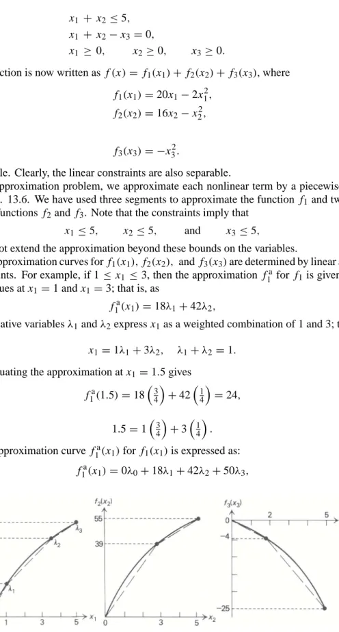
The objective function is now written as f(x)= f1(x1)+ f2(x2)+ f3(x3), where f1(x1)=20x1−2x12,
f2(x2)=16x2−x22, and
f3(x3)= −x32.
Thus it is separable. Clearly, the linear constraints are also separable.
To form the approximation problem, we approximate each nonlinear term by a piecewise-linear curve, as pictured in Fig. 13.6. We have used three segments to approximate the function f1 and two segments to approximate the functions f2and f3. Note that the constraints imply that
x1≤5, x2≤5, and x3≤5,
so that we need not extend the approximation beyond these bounds on the variables.
The dashed approximation curves for f1(x1), f2(x2), and f3(x3)are determined by linear approximation between breakpoints. For example, if 1≤ x1 ≤3, then the approximation fa
1 for f1is given by weighting the function’s values at x1=1 and x1 =3; that is, as
f1a(x1)=18λ1+42λ2,
where the nonnegative variablesλ1andλ2express x1 as a weighted combination of 1 and 3; thus,
x1=1λ1+3λ2, λ1+λ2 =1. For instance, evaluating the approximation at x1=1.5 gives
f1a(1.5)=18 3 4 +42 1 4 =24, since 1.5=134+314. The overall approximation curve f1a(x1)for f1(x1)is expressed as:
f1a(x1)=0λ0+18λ1+42λ2+50λ3,
(1)
where
x1 =0λ0+1λ1+3λ2+5λ3, (2)
λ0+λ1+λ2+λ3=1,
λj ≥0 (j =1,2,3,4),
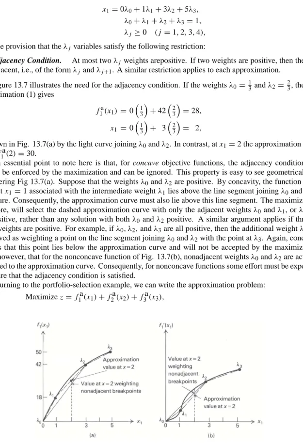
with the provision that theλj variables satisfy the following restriction:
Adjacency Condition. At most twoλj weights arepositive. If two weights are positive, then they are
adjacent, i.e., of the formλj andλj+1. A similar restriction applies to each approximation.
Figure 13.7 illustrates the need for the adjacency condition. If the weightsλ0 = 13 andλ2 = 23, then the approximation (1) gives f1a(x1) = 0 1 3 +42 2 3 =28, x1 = 0 1 3 + 323= 2,
as shown in Fig. 13.7(a) by the light curve joiningλ0andλ2. In contrast, at x1 =2 the approximation curve gives f a1(2)=30.
An essential point to note here is that, for concave objective functions, the adjacency condition will always be enforced by the maximization and can be ignored. This property is easy to see geometrically by considering Fig 13.7(a). Suppose that the weightsλ0 andλ2 are positive. By concavity, the function value of 18 at x1 =1 associated with the intermediate weightλ1lies above the line segment joiningλ0 andλ2in
the figure. Consequently, the approximation curve must also lie above this line segment. The maximization, therefore, will select the dashed approximation curve with only the adjacent weightsλ0 andλ1, orλ1 and
λ2, positive, rather than any solution with bothλ0 andλ2 positive. A similar argument applies if three or more weights are positive. For example, ifλ0, λ2,andλ3 are all positive, then the additional weightλ3can be viewed as weighting a point on the line segment joiningλ0andλ2with the point atλ3. Again, concavity implies that this point lies below the approximation curve and will not be accepted by the maximization. Note, however, that for the nonconcave function of Fig. 13.7(b), nonadjacent weightsλ0andλ2are actually preferred to the approximation curve. Consequently, for nonconcave functions some effort must be expended to ensure that the adjacency condition is satisfied.
Returning to the portfolio-selection example, we can write the approximation problem: Maximize z = f a1(x1)+ f a2(x2)+ f a3(x3),
13.5 Separable Programming 423
subject to:
x1 + x2 ≤5,
x1 + x2 − x3 =0,
x1 ≥0, x2 ≥0, x3 ≥0,
in terms of weighting variables λi j. Here we use the first subscript i to denote the weights to attach to variable i . The weightsλ0, λ1, λ2, andλ3 used above for variable x1 thus becomeλ10, λ11, λ12, andλ13. The formulation is:
Maximize z = 0λ10+18λ11+42λ12+50λ13+0λ20+39λ21+55λ22−0λ30−4λ31−25λ32, subject to: 0λ10 + 1λ11 + 3λ12 + 5λ13 +0λ20 + 3λ21 + 5λ22 ≤5, 0λ10 + 1λ11 + 3λ12 + 5λ13 +0λ20 + 3λ21 + 5λ22 −0λ30 − 2λ31 − 5λ32 =0, λ10 + λ11 + λ12 + λ13 =1 λ20 + λ21 + λ22 =1 λ30 + λ31 + λ32 =1
λi j ≥0, for all i and j.
Since each of the functions f1(x1),f2(x2),and f3(x3)is concave, the adjacency condition can be ignored and the problem can be solved as a linear program. Solving by the simplex method gives an optimal objective value of 44 withλ11 = λ12 =0.5, λ21 =1, andλ32 = 1 as the positive variables in the optimal solution. The corresponding values for the original problem variables are:
x1=(0.5)(1)+(0.5)(3)=2, x2=3, and x3 =5. This solution should be contrasted with the true solution
x1 = 73, x2 = 83, x3 =5, and f(x1,x2,x3)=4613, which we derive in Section 13.7.
Note that the approximation problem has added severalλvariables and that one weighting constraint in (2) is associated with each xj variable. Fortunately, these weighting constraints are of a special generalized
upper-bounding type, which add little to computational effort and keep the number of effective constraints essentially unchanged. Thus, the technique can be applied to fairly large nonlinear programs, depending of course upon the capabilities of available linear-programming codes.
Once the approximation problem has been solved, we can obtain a better solution by introducing more breakpoints. Usually more breakpoints will be added near the optimal solution given by the original approx-imation.
Adding a single new breakpoint at x1 = 2 leads to an improved approximation for this problem with a
linear-programming objective value of 46 and
x1 =2, x2 =3, and x3 =5.
In this way, an approximate solution can be found as close as desired to the actual solution.
General Procedure
The general problem must be approached more carefully, since linear programming can give nonadjacent weights. The procedure is to express each variable∗in terms of breakpoints, e.g., as above
x1=0λ10+1λ11+3λ12+5λ13,
∗Variables that appear in the model in only a linear fashion should not be approximated and remain as x
and then use these breakpoints to approximate the objective function and each constraint, giving the approx-imation problem: Maximize n X j=1 f aj (xj), subject to: (3) n X j=1 gai j(xj)≤bi (i=1,2, . . . ,m).
If each original function fj(xj)is concave and each gi j(xj)convex,†then theλi j version is solved as a linear
program. Otherwise, the simplex method is modified to enforce the adjacency condition. A natural approach is to apply the simplex method as usual, except for a modified rule that maintains the adjacency condition at each step. The alteration is:
Restricted-Entry Criterion. Use the simplex criterion, butdo not introduce aλi kvariable into the basis unless there is only oneλi j variable currently in the basis and it is of the formλi,k−1orλi,k+1, i.e.,it is adjacent toλi k.
Note that, when we use this rule, the optimal solution may contain a nonbasic variableλi k that would ordinarily be introduced into the basis by the simplex method (since its objective cost in the canonical form is positive), but is not introduced because of the restricted-entry criterion. If the simplex method would choose a variable to enter the basis that is unacceptable by the restricted-entry rule, then we choose the next best variable according to the greatest positive reduced cost.
An attractive feature of this procedure is that it can be obtained by making very minor modifications to any existing linear-programming computer code. As a consequence, most commercial linear-programming packages contain a variation of this separable-programming algorithm. However, the solution determined by this method in the general case can only be shown to be a localoptimum to the approximation problem (3).
Inducing Separability
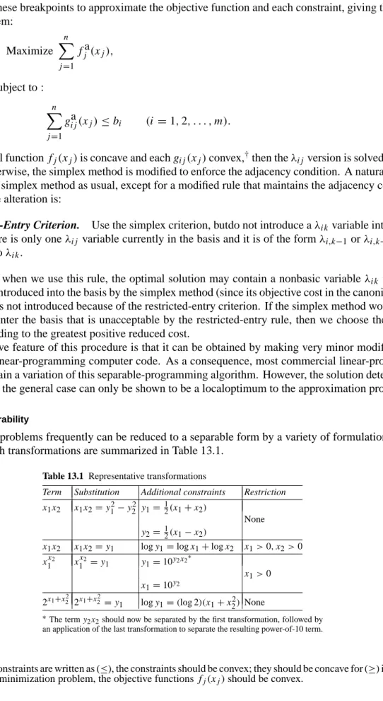
Nonseparable problems frequently can be reduced to a separable form by a variety of formulation tricks. A number of such transformations are summarized in Table 13.1.
Table 13.1 Representative transformations
Term Substitution Additional constraints Restriction x1x2 x1x2=y12−y22 y1= 12(x1+x2)
None y2= 1
2(x1−x2)
x1x2 x1x2=y1 log y1=log x1+log x2 x1>0,x2>0 xx2 1 x x2 1 =y1 y1=10y2x2 ∗ x1>0 x1=10y2
2x1+x22 2x1+x22 =y1 log y1=(log 2)(x1+x22) None
∗The term y
2x2should now be separated by the first transformation, followed by an application of the last transformation to separate the resulting power-of-10 term.
†Because the constraints are written as (≤), the constraints should be convex; they should be concave for (≥) inequalities.
13.6 Linear Approximations of Nonlinear Programs 425
To see the versatility of these transformations, suppose that the nonseparable term x1x22/(1+x3)appears
either in the objective function or in a constraint of a problem. Letting y1 =1/(1+x3), the term becomes x1x22y1. Now if x1 >0,x22 >0, and y1 >0 over the feasible region, thenletting y2 =x1x22y1, the original term is replaced by y2and the separable constraints
y1 = 1 1 + x3 and
log y2 =log x1+log x22+log y1
are introduced. If the restrictions x1>0, x22>0, y1 >0 arenot met, we may let y2=x1x22, substitute y1y2 for the original term, and append the constraints:
y1 = 1
1 + x3, y2 =x1x
2 2.
The nonseparable terms y1y2and x1x22can now be separated using the first transformation in Table 13.1 (for the last expression, let x22replace x2in the table).
Using the techniques illustrated by this simple example, we may, in theory, state almost any optimization problem as a separable program. Computationally, though, the approach is limited since the number of added variables and constraints may make the resulting separable program too large to be manageable.
13.6 LINEAR APPROXIMATIONS OF NONLINEAR PROGRAMS
Algebraic procedures such as pivoting are so powerful for manipulating linear equalities and inequalities that many nonlinear-programming algorithms replace the given problem by an approximating linear problem. Separable programming is a prime example, and also one of the most useful, of these procedures. As in separable programming, these nonlinear algorithms usually solve several linear approximations by letting the solution of the last approximation suggest a new one.
By using different approximation schemes, this strategy can be implemented in several ways. This section introduces three of these methods, all structured to exploit the extraordinary computational capabilities of the simplex method and the wide-spread availability of its computer implementation.
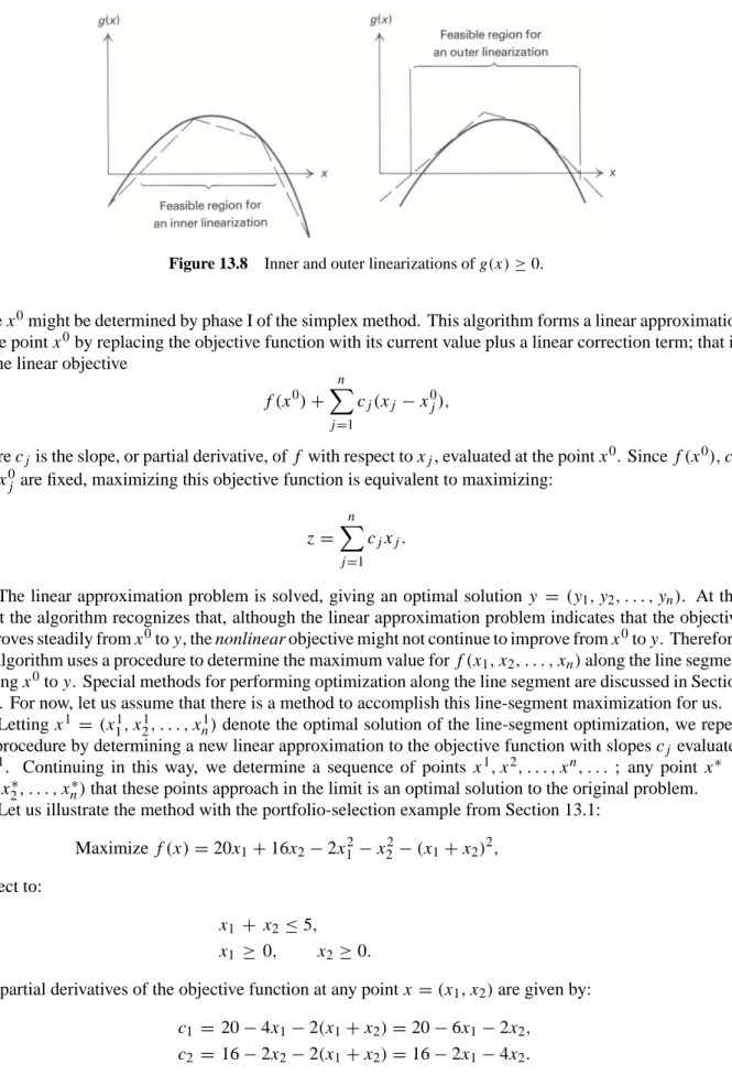
There are two general schemes for approximating nonlinear programs. The last section used linear ap-proximation for separable problems by weighting selected values of each function. This method is frequently referred to as inner linearization since, as shown in Fig. 13.8 when applied to a convex programming prob-lem (i.e., constraints gi(x) ≥ 0 with gi concave, or gi(x) ≤ 0 with gi convex), the feasible region for the
approximating problem lies inside that of the original problem. In contrast, other approximation schemes use slopes to approximate each function. These methods are commonly referred to as outer linearizations since, for convex-programming problems, the feasible region for the approximating problem encompasses that of the original problem. Both approaches are illustrated further in this section.
Frank–Wolfe Algorithm Let x0 =(x0 1,x 0 2, . . . ,x 0
n)be any feasible solution to a nonlinear program with linear constraints:
Maximize f(x1,x2, . . . ,xn), subject to: n X j=1 ai jxj ≤bi (i =1,2, . . . ,m), xj ≥0 (j =1,2, . . . ,n).
Figure 13.8 Inner and outer linearizations of g(x)≥0.
Here x0might be determined by phase I of the simplex method. This algorithm forms a linear approximation at the point x0by replacing the objective function with its current value plus a linear correction term; that is, by the linear objective
f(x0)+ n X
j=1
cj(xj −x0j),
where cj is the slope, or partial derivative, of f with respect to xj, evaluated at the point x0. Since f(x0),cj,
and x0j are fixed, maximizing this objective function is equivalent to maximizing:
z = n X
j=1
cjxj.
The linear approximation problem is solved, giving an optimal solution y = (y1,y2, . . . ,yn). At this
point the algorithm recognizes that, although the linear approximation problem indicates that the objective improves steadily from x0to y, the nonlinear objective might not continue to improve from x0to y. Therefore, the algorithm uses a procedure to determine the maximum value for f(x1,x2, . . . ,xn)along the line segment
joining x0to y. Special methods for performing optimization along the line segment are discussed in Section 13.9. For now, let us assume that there is a method to accomplish this line-segment maximization for us.
Letting x1 = (x1
1,x21, . . . ,xn1)denote the optimal solution of the line-segment optimization, we repeat
the procedure by determining a new linear approximation to the objective function with slopes cj evaluated
at x1. Continuing in this way, we determine a sequence of points x1,x2, . . . ,xn, . . . ; any point x∗ = (x1∗,x2∗, . . . ,xn∗)that these points approach in the limit is an optimal solution to the original problem.
Let us illustrate the method with the portfolio-selection example from Section 13.1: Maximize f(x)=20x1+16x2−2x12−x22−(x1+x2)2,
subject to:
x1 + x2 ≤5,
x1 ≥ 0, x2≥0.
The partial derivatives of the objective function at any point x =(x1,x2)are given by: c1 = 20−4x1−2(x1+x2)=20−6x1−2x2,
13.6 Linear Approximations of Nonlinear Programs 427
Suppose that the initial point is x0 =(0,0). At this point c1 =20 and c2=16 and the linear approximation
uses the objective function 20x1+16x2. The optimal solution to this linear program is y1 = 5, y2 = 0, and the line-segment optimization is made on the line joining x0 = (0,0) to y = (5,0); that is, with
0≤x1 ≤5,x2 =0. The optimal solution can be determined to be x1=313,x2 =0, so that the procedure is repeated from x1 =(31
3,0).
The partial derivatives are now c1 = 0,c2 = 91
3, and the solution to the resulting linear program of maximizing 0x1+91
3x2is y1 =0,y2=5. The line segment joining x
1and y is given by
x1 = θy1+(1−θ)x11=313(1−θ),
x2 = θy2+(1−θ)x21=5θ,
asθ varies between 0 and 1. The optimal value ofθ over the line segment isθ = 7
15, so that the next point is:
x12= 10 3 8 15 =17 9 and x 2 2 =2 1 3.
Figure 13.9 illustrates these two steps of the algorithm and indicates the next few points x4,x5, and x6 that it generates.
Figure 13.9 Example of the Frank–Wolfe algorithm.
The Frank–Wolfe algorithm is convenient computationally because it solves linear programs with the same constraints as the original problem. Consequently, any structural properties of these constraints are
available when solving the linear programs. In particular, network-flow techniques or large-scale system methods can be used whenever the constraints have the appropriate structure. Also, note from Fig. 13.9 that the points x1,x2,x3, . . . oscillate. The even-numbered points x2,x4,x6, . . . lie on one line directed toward the optimal solution, and the odd-numbered points x1,x3,x5, . . . , lie on another such line. This general tendency of the algorithm slows its convergence. One approach for exploiting this property to speed convergence is to make periodic optimizations along the line generated by every other point xk+2and xkfor some values of k.
MAP (Method of Approximation Programming)
The Frank–Wolfe algorithm can be extended to general nonlinear programs by making linear approximations to the constraints as well as the objective function. When the constraints are highly nonlinear, however, the solution to the approximation problem can become far removed from feasible region since the algorithm permits large moves from any candidate solution. The Method of Approximation Programming (MAP) is a simple modification of this approach that limits the size of any move. As a result, it is sometimes referred to as a small-step procedure.
Let x0 =(x0
1,x 0
2, . . . ,xn0)be any candidate solution to the optimization problem:
Maximize f(x1,x2, . . . ,xn), subject to:
gi(x1,x2, . . . ,xn)≤0 (i=1,2, . . . ,m).
Each constraint can be linearized, using its current value gi(x0)plus a linear correction term, as:
ˆ gi(x)=gi(x0)+ n X j=1 ai j(xj −x0j)≤0,
where ai j is the partial derivative of constraint gi with respect to variable xj evaluated at the point x0. This
approximation is a linear inequality, which can be written as:
n X j=1 ai jxj ≤b0i ≡ n X j=1 ai jx0j −gi(x0),
since the terms on the righthand side are all constants.
The MAP algorithm uses these approximations, together with the linear objective-function approximation, and solves the linear-programming problem:
Maximize z = n X j=1 cjxj, subject to: n X j=1 ai jxj ≤bi0 (i=1,2, . . . ,m), (4) x0j −δj ≤ xj ≤x0j +δj (j =1,2, . . . ,n).
The last constraints restrict the step size; they specify that the value for xj can vary from x0j by no more than
the user-specified constantδj.
When the parametersδj are selected to be small, the solution to this linear program is not far removal
13.6 Linear Approximations of Nonlinear Programs 429
Frank–Wolfe algorithm is not worth the slightly improved solution that it provides. MAP operates on this premise, taking the solution to the linear program (4) as the new point x1. The partial-derivative data ai j,bi,
and cj is recalculated at x1, and the procedure is repeated. Continuing in this manner determines points x1,x2, . . . ,xk, . . .and as in the Frank–Wolfe procedure, any point x∗= (x∗
1,x ∗ 2, . . . ,x
∗
n)that these points
approach in the limit is considered a solution.
Steps of the MAP Algorithm
STEP (0): Let x0 = (x0
1,x02, . . . ,xn0)be any candidate solution, usually selected to be feasible or
near-feasible. Set k =0.
STEP (1): Calculate cj and ai j(i = 1,2, . . . ,m), the partial derivatives of the objective function and
constraints evaluated at xk =(xk 1,x k 2, . . . ,x k n). Let bki =ai jx k−g i(xk).
STEP (2): Solve the linear-approximation problem (4) with bki and xkj replacing b0i and x0j, respectively. Let xk+1=(xk+1
1 ,x
k+1 2 , . . . ,x
k+1
n )be its optimal solution. Increment k to k+1 and return to
STEP 1.
Since many of the constraints in the linear approximation merely specify upper and lower bounds on the decision variables xj, the bounded-variable version of the simplex method is employed in its solution. Also,
usually the constantsδj are reduced as the algorithm proceeds. There are many ways to implement this idea.
One method used frequently in practice, is to reduce eachδj by between 30 and 50 percent at each iteration.
To illustrate the MAP algorithm, consider the problem: Maximize f(x)= [(x1−1)2+x22], subject to:
g1(x) = x12+6x2− 36≤0,
g2(x) = −4x1+ x22−2x2 ≤0,
x1 ≥0, x2≥0.
The partial derivatives evaluated at the point x =(x1,x2)are given by: c1 =2x1−2, c2 =2x2,
a11 =2x1, a12 =6,
a21 = −4, a22 =2x2−2.
Since linear approximations of any linear function gives that function again, no data needs to be calculated for the linear constraints x1≥0 and x2≥0.
Using these relationships and initiating the procedure at x0 = (0,2)withδ1 =δ2 =2 gives the
linear-approximation problem: Maximize z= −2x1+4x2, subject to: 0x1+6x2 ≤ 0(0)+6(2)−(−24)=36, −4x1+2x2 ≤ −4(0)+2(2)− 0 =4. −2≤ x1≤2, 0≤ x2≤4.
The feasible region and this linear approximation are depicted in Fig. 13.10. Geometrically, we see that the optimalsolution occurs at x11 =1,x21 = 4. Using this point and reducing bothδ1andδ2 to 1 generates the new approximation:
Maximize z=0x1+8x2,
subject to:
2x1+6x2 ≤ 2(1)+6(4)−(−11)=37, −4x1+6x2 ≤ −4(1)+6(4)− (4)=16,
0 ≤ x1 ≤2, 3≤x2≤5.
The solution indicated in Fig. 13.10 occurs at x12 =2, x2
2 =4.
Figure 13.10 Example of the MAP algorithm.
If the procedure is continued, the points x3,x4, . . . that it generates approach the optimal solution x∗ shown in Fig. 13.10. As a final note, let us observe that the solution x1is not feasible for the linear program that was constructed by making linear approximations at x1. Thus, in general, both Phase I and Phase II of the simplex method may be required to solve each linear-programming approximation.
13.6 Linear Approximations of Nonlinear Programs 431
Generalized Programming
This algorithm is applied to the optimization problem of selecting decision variables x1,x2, . . . ,xn from a
region C to:
Maximize f(x1,x2, . . . ,xn),
subject to:
gi(x1,x2, . . . ,xn)≤0 (i=1,2, . . . ,m).
The procedure uses inner linearization and extends the decomposition and column-generation algorithms introduced in Chapter 12. When the objective function and constraints gi are linear and C consists of the
feasible points for a linear-programming subproblem, generalized programming reduces to the decomposition method.
As in decomposition, the algorithm starts with k candidate solutions xj = (x1j,x2j, . . . ,xnj) for j =
1,2, . . . ,k, all lying the region C. Weighting these points byλ1, λ2, . . . , λkgenerates the candidate solution:
xi =λ1xi1+λ2xi2+ · · · +λkxik (i =1,2, . . . ,n). (5)
Any choices can be made for the weights as long as they are nonnegative and sum to one. The ‘‘best’’ choice is determined by solving the linear-approximation problem in the variablesλ1, λ2, . . . , λk:
Maximize λ1f(x1)+λ2f(x2)+ · · · +λkf(xk), Optimal
subject to: shadow
prices λ1g1(x1)+λ2g1(x2)+ · · · +λkg1(xk)≤0, y1 ... ... ... ... (6) λ1gm(x1)+λ2gm(x2)+ · · · +λkgm(xk)≤0, ym λ1 +λ2 + λk=1. σ λj ≥0 (j =1,2, . . . ,k).
The coefficients f(xj)and gi(xj) of the weightsλj in this linear program are fixed by our choice of the
candidate solutions x1,x2, . . . ,xk. In this problem, the original objective function and constraints have been replaced by linear approximations. When x is determined from expression (5) by weighting the points
x1,x2, . . . ,xkby the solution of problem (6), the linear approximations at x are given by applying the same weights to the objective function and constraints evaluated at these points; that is,
fa(x)=λ1f(x1)+λ2f(x2)+ · · · +λkf(xk)
and
gai(x)=λ1gi(x1)+λ2gi(x2)+ · · · +λkgi(xk).
The approximation is refined by applying column generation to this linear program. In this case, a new column with coefficients f(xk+1),g1(xk+1), . . . ,gm(xk+1)is determined by the pricing-out operation:
v=Max[f(x)−y1g1(x)−y2g2(x)− · · · −ymgm(x)],
subject to:
x ∈C.
This itself is a nonlinear programming problem but without the gi constraints. Ifv−σ ≤ 0, then no new
givingvdetermines a new column to be added to the linear program (6) and the procedure continues. The optimal weightsλ∗1, λ∗2, . . . , λ∗kto the linear program provide a candidate solution
xi∗=λ∗1xi1+λ∗2xi2+ · · · +λ∗kxik
to the original optimization problem. This candidate solution is most useful when C is a convex set and each constraint is convex, for then xi∗is a weighted combination of points x1,x2, . . . ,xkin C and thus belongs to
C; and, since linear interpolation overestimates convex functions,
gi(x∗)≤λ1∗gi(x1)+λ∗2gi(x2)+ · · · +λ∗kgi(xk).
The righthand side is less than or equal to zero by the linear-programming constraints; hence, gi(x∗) ≤ 0
and x∗is a feasible solution to the original problem.
As an illustration of the method, consider the nonlinear program: Maximize f(x)=x1−(x2−5)2+9,
subject to:
g(x)=x12 + x22−16≤0, x1 ≥ 0, x2 ≥0.
We let C be the region with x1≥0 and x2≥0, and start with the three points x1 =(0,0),x2 =(5,0), and x3 =(0,5)from C. The resulting linear approximation problem:
Maximize z = −16λ1−11λ2+9λ3, Optimal
subject to: shadow
prices
−16λ1+9λ2+9λ3 ≤0, y=1
λ1+λ2+λ3=1, σ =0
λ1 ≥0, λ2 ≥0, λ2 ≥0,
is sketched in Fig. 13.11, together with the original problem. The feasible region for the approximation problem is given by plotting the points defined by (5) that correspond to feasible weights in this linear program.
Figure 13.11 An example of generalized programming. The solution to the linear program is:
λ∗ 1 =0.36, λ ∗ 2=0, and λ ∗ 3 =0.64,
13.7 Quadratic Programming 433
or
x∗=0.36(0,0)+0.64(0,5)=(0,3.2).
The nonlinear programming subproblem is:
Maximize[f(x)−yg(x)] =x1−(x2−5)2−yx12−yx 2
2+16y+9, subject to:
x1≥0, x2 ≥0.
For y >0 the solution to this problem can be shown to be x1 =1/(2y)and x2 =5/(1+y), by setting the
partial derivatives of f(x)−yg(x), with respect to x1and x2, equal to zero.
In particular, the optimal shadow price y=1 gives the new point x4 = 1 2,2 1 2 . Since f(x4)=314 and g(x4)= −91
2, the updated linear programming approximation is: Maximize z = −16λ1−11λ2+9λ3+31
4λ4, Optimal
subject to: shadow
prices −16λ1+9λ2+9λ3−91 2λ4 ≤0, y = 23 74 λ1+λ2+λ3+λ4=1, σ = 45974 λj ≥0 (j =(1,2,3,4).
The optimal solution hasλ3andλ4basic withλ∗3 = 1937, λ∗4 = 1837. The corresponding value for x is:
x∗ = λ∗3(0,5)+λ∗4 1 2,2 1 2 = 19 37(0,5)+ 18 37 1 2,2 1 2 = 9 37,3 29 37 .
As we continue in this way, the approximate solutions will approach the optimal solution x1 = 1.460 and
x2 =3.724 to the original problem.
We should emphasize that the generalized programming is unlike decomposition for linear programs in that it does not necessarily determine the optimal solution in a finite number of steps. This is true because nonlinearity does not permit a finite number of extreme points to completely characterize solutions to the subproblem.
13.7 QUADRATIC PROGRAMMING
Quadratic programming concerns the maximization of a quadratic objective function subject to linear con-straints, i.e., the problem:
Maximize f(x)= n X j=1 cjxj +12 n X j=1 n X k=1 qj kxjxk, subject to: n X j=1 ai jxj ≤ bi (i =1,2, . . . ,m), xj ≥ 0 (j=1,2, . . . ,n).
The data cj,ai j, and bi are assumed to be known, as are the additional qj kdata. We also assume the
sym-metry condition qj k =qk j. This condition is really no restriction, since qj kcan be replaced by21(qj k+qk j).
The symmetry condition is then met, and a straightforward calculation shows that the old and new qj k
simplify later calculations; if desired, it can be incorporated into the qj k coefficients. Note that, if every qj k =0, then the problem reduces to a linear program.
The first and third examples of Section 13.1 show that the quadratic-programming model arises in con-strained regression and portfolio selection. Additionally, the model is frequently applied to approximate problems of maximizing general functions subject to linear constraints.
In Chapter 4 we developed the optimality conditions for linear programming. Now we will indicate the analogous results for quadratic programming. The motivating idea is to note that, for a linear objective function f(x)= n X j=1 cjxj,
the derivative (i.e., the slope or marginal return) of f with respect to xjis given by cj, whereas, for a quadratic
program, the slope at a point is given by
cj + n X k=1
qj kxk.
The quadratic optimality conditions are then stated by replacing every cjin the linear-programming optimality
conditions by cj +Pnk=1qj kxk. (See Tableau 1.)
Tableau 1 Optimality conditions
Linear program Quadratic program Primal feasibility n P j=1 ai jxj ≤bi, n P j=1 ai jxj ≤bi, xj ≥0 xj ≥0 Dual feasibility m P i=1 yiai j ≥cj, m P i=1 yiai j ≥cj+ n P k=1 qj kxk, yi ≥0 yi ≥0 Complementary slackness yi " bi− n P j=1 ai jxj # =0, yi " bi− n P j=1 ai jxj # =0, " m P i=1 yiai j−cj # xj =0 " m P i=1 yiai j−cj− n P k=1 qj kxk # xj =0
Note that the primal and dual feasibility conditions for the quadratic program are linear inequalities in nonnegative variables xj and yi. As such, they can be solved by the Phase I simplex method. A simple
modification to that method will permit the complementary-slackness conditions to be maintained as well. To discuss the modification, let us introduce slack variables si for the primal constraints and surplus variables vj for the dual constraints; that is,
si =bi − n X j=1 ai jxj, vj = m X i=1 yiai j −cj − n X k=1 qj kxk.
Then the complementary slackness conditions become:
13.8 Quadratic Programming 435
and
vjxj =0 (j =1,2, . . . ,n).
The variables yi and si are called complementary, as are the variablesvj and xj. With this notation, the
technique is to solve the primal and dual conditions by the Phase I simplex method, but not to allow any complementary pair of variables to appear in the basis both at the same time. More formally, the Phase I simplex method is modified by the:
Restricted-Entry Rule. Never introduce avariable into the basis if its complementary variable is already a member of the basis, even if the usual simplex criterion says to introduce the variable.
Otherwise, the Phase I procedure is applied as usual. If the Phase I procedure would choose a variable to enter the basis that is unacceptable by the restricted-entry rule, then we choose the next best variable according to the greatest positive reduced cost in the Phase I objective function.
An example should illustrate the technique. Again, the portfolio-selection problem of Section 13.1 will be solved withθ =1; that is,
Maximize f(x)=20x1+16x2−2x12−x22−(x1+x2)2,
subject to:
x1+x2 ≤5,
x1 ≥0, x2 ≥0.
Expanding(x1+x2)2as x12+2x1x2+x22 and incorporating the factor12, we rewrite the objective function as:
Maximize f(x)=20x1+16x2+ 1
2(−6x1x1−4x2x2−2x1x2−2x2x1), so that q11 = −6,q12 = −2, q21 = −2, q22 = −4, and the optimality conditions are:
s1=5−x1−x2, (Primal constraint) v1 =y1−20+6x1+2x2 v2 =y1−16+2x1+4x2 (Dual constraints) x1, x2, s1, v1, v2, y1≥0, (Nonnegativity) y1s1 =0, v1x1 =0, v2x2 =0. (Complementary slackness)
Letting s1be the basic variable isolated in the first constraint and adding artificial variables a1and a2in the second and third constraints, the Phase I problem is solved in Table 13.2.
For this problem, the restricted-entry variant of the simplex Phase I procedure has provided the optimal solution. It should be noted, however, that the algorithm will not solve every quadratic program. As an example, consider the problem:
Maximize f(x1,x2)= 1 4(x1−x2) 2, subject to: x1+x2≤5, x1≥0, x2 ≥0.
As the reader can verify, the algorithm gives the solutionx1 = x2 = 0. But this solution is not even a
local optimum, since increasing either x1or x2increases the objective value.
It can be shown, however, that the algorithm does determine an optimal solution if f(x)is strictly concave for a maximization problem or strictly convex for a minimization problem. For the quadratic problem, f(x)
is strictly concave whenever
n X i=1 n X j=1
αiqi jαj <0 for every choice ofα1, α2, . . . , αn,
such that someαj 6= 0. In this case, the matrix of coefficients(qi j) is called negative definite. Thus the
algorithm will always work for a number of important applications including the least-square regression and portfolio-selection problems introduced previously.
Table 13.2 Solving a quadratic program. Basic Current variables values x1 x2 s1 y1∗ v1 v2 a1 a2 s1 5 1 1 1 0 0 0 ← a1 20 6 2 1 −1 0 1 a2 16 2 4 1 0 −1 1 (−w) 36 8 6 2 −1 −1 ↑ Basic Current variables values x1 x2 s1 y1∗ v1∗ v2 a1 a2 ← s1 53 23 1 −16 16 0 −16 x1 103 1 13 16 −16 0 16 a2 283 103 23 13 −1 −13 1 (−w) 28 3 10 3 2 3 1 3 0 − 4 3 ↑ Basic Current variables values x1 x2 s1 y1 v1∗ v ∗ 2 a1 a2 x2 52 1 32 −14 14 0 −14 x1 52 1 −12 14 −14 0 14 ← a2 1 −5 23 −12 −1 12 1 (−w) 1 −5 32 −1 2 0 − 1 2 ↑ Basic Current variables values x1 x2 s1∗ y1 v1∗ v ∗ 2 a1 a2 x2 83 1 23 16 −1 6 − 1 6 1 6 x1 73 1 1 3 − 1 6 1 6 1 6 − 1 6 y1 23 103 1 13 −23 13 23 (−w) 0 0 0 1 −1 −1 * Starred variables cannot be introduced into the basis since their complementary variable is in the basis
.
13.8 UNCONSTRAINED MINIMIZATION AND SUMT
Conceptually, the simplest type of optimization is unconstrained. Powerful solution techniques have been developed for solving these problems, which are based primarily upon calculus, rather than upon algebra and pivoting, as in the simplex method. Because the linear-programming methods and unconstrained-optimization techniques are so efficient, both have been used as the point of departure for constructing more general-purpose nonlinear-programming algorithms. The previous sections have indicated some of the algorithms using the linear-programming-based approach. This section briefly indicates the nature of the unconstrained-optimization approaches by introducing algorithms for unconstrained maximization and showing how they might be used for problems with constraints.
Unconstrained Minimization
Suppose that we want to maximize the function f(x)of n decision variables x = (x1,x2, . . . ,xn)and that
this function is differentiable. Let∂f/∂xj denote the partialderivative of f with respect to xj, defined by