Stability of Feature Selection Algorithms
Alexandros Kalousis, Julien Prados, Melanie Hilario
University of Geneva, Computer Science Department
Rue General Dufour 24, 1211 Geneva 4, Switzerland
{
kalousis, prados, hilario
}
@cui.unige.ch
Abstract
With the proliferation of extremely high-dimensional data, feature selection algorithms have become indispens-able components of the learning process. Strangely, despite extensive work on the stability of learning algorithms, the stability of feature selection algorithms has been relatively neglected. This study is an attempt to fill that gap by quanti-fying the sensitivity of feature selection algorithms to vari-ations in the training set. We assess the stability of ture selection algorithms based on the stability of the fea-ture preferences that they express in the form of weights-scores, ranks, or a selected feature subset. We examine a number of measures to quantify the stability of feature pref-erences and propose an empirical way to estimate them. We perform a series of experiments with several feature selec-tion algorithms on a set of proteomics datasets. The ex-periments allow us to explore the merits of each stability measure and create stability profiles of the feature selection algorithms. Finally we show how stability profiles can sup-port the choice of a feature selection algorithm.
1 Introduction
High dimensional datasets are becoming more and more abundant in classification problems. A variety of feature se-lection methods have been developed to tackle the issue of high dimensionality. The major challenge in these applica-tions is to extract a set of features, as small as possible, that accurately classifies the learning examples.
A relatively neglected issue in the work on high dimen-sional problems, and in general in problems requiring fea-ture selection, is the stability of the feafea-ture selection meth-ods used. Stability, defined as the sensitivity of a method to variations in the training set, has been extensively studied with respect to the learning algorithm itself. We propose to investigate how different subsamples of a training set affect a method’s assessment of a feature’s importance and conse-quently the final set of selected features.
The stability of classification algorithms was examined by Turney [11] who proposed a measure based on the agree-ment of classification models produced by an algorithm when trained on different training sets. He defined the agreement of two classification models as the probability that they will produce the same predictions over all possible instances drawn from a probability distributionP(X). Note
that instances are drawn fromP(X)and not fromP(X, C), the joint probability distribution of class and training in-stances; the underlying reason is that the agreement of two concepts—classification models—should be examined in all possible input worlds. In order to estimate stability he suggested usingm×2-fold cross-validation. In each of the m repetitions of cross-validation a classification model is produced from each one of the two folds. The two mod-els are then tested on artificial instances drawn by sampling fromP(X)and their agreement is computed. The final
esti-mation of stability is the average agreement over allmruns. Related to the notion of stability is the bias-variance de-composition of the error of classification algorithms, [4, 1]. The variance term quantifies instability of the classification algorithm in terms of classification predictions. Variance measures the percentage of times that the predictions of dif-ferent classification models, learned from difdif-ferent training sets, for a given instance are different from the typical (av-erage) prediction. Bias-variance decomposition is usually done via bootstrapping, where part of the data is kept as a hold-out test set and the remainder is used to create different training sets by using sampling with replacement. The final estimation of variance is also the average over the different bootstrap samples.
In both approaches described above, the predictions of the classification models are crucial in quantifying the sen-sitivity of classification algorithms to changes in the train-ing sets (note that both approaches can also be used for er-ror estimation which is then tightly coupled with the sta-bility analysis). However when one wants to examine only feature selection algorithms without involving a classifica-tion algorithm, the above methods do not apply. Typical feature selection algorithms do not construct classification
models and thus cannot provide classification predictions. They usually output what we call a feature preference state-ment (for conciseness, feature preference); this can take the form of a subset of selected features, or alternatively of a weighting-scoring or a ranking of the features, based on which a small set of features can be selected (either by specifying a threshold or asking for a specific number of features). A classification algorithm should then be applied on the selected feature set to produce a classification model. If we used the stability estimation methods described above to the combined feature selection and classification algo-rithms, we would be measuring their joint sensitivity to training set variations and we would have no way to delimit the (in)stability the feature selection algorithm from that of the classification algorithm.
To address this difficulty we introduce the notion of pref-erential stability, i.e., the stability of the feature preferences produced by a feature selection algorithm, to quantify its sensitivity to differences in training sets drawn from the same distribution. The same approach can in fact be used to measure the preferential stability of any classification algo-rithm that produces models from which weightings or rank-ings of the features can be extracted, e.g. linear discrimina-tion algorithms.
Stability, as introduced in [11], and the bias-variance de-composition frameworks are not able to accurately quantify preferential stability. It is possible that different training samples lead to really different feature sets which however yield the same prediction patterns. This can be especially true when the initial features have a high level of redun-dancy which is not handled in a principled way by the algo-rithms used.
The motivation for investigating the stability of feature selection algorithms came from the need to provide appli-cation domain experts with quantified evidence that the se-lected features are relatively robust to variations in the train-ing data. This need is particularly crucial in proteomics ap-plications. In mass spectrometry based diagnosis, for in-stance, training data (protein mass spectra) are character-ized by high dimensionality and the goal is to output a small set of highly discriminatory features (protein biomarkers) on which biomedical experts will subsequently invest con-siderable time and research effort. Domain experts tend to have less confidence in feature sets that change radically with slight variations in the training data. Data miners have to convince them not only of the predictive potential but also of the relative stability of the proposed features or biomark-ers.
The rest of the paper is organized as follows: in Section 2 we introduce measures of stability that can be applied to any feature selection algorithm that outputs a feature preference as defined above; we also show how we can empirically es-timate these measures. In Section 3 we describe the
experi-mental setup, the datasets used, and the feature selection al-gorithms included in the study; in Section 4 we present the results of the experiments, investigate the behavior of the different stability measures and establish the stability pro-files of the chosen feature selection algorithms; in Section 5 we examine together classification performance and stabil-ity of feature preferences, and suggest how we can exploit the latter to support the choice of the appropriate feature selection algorithm; finally we conclude in Section 6.
2 Stability
The generic model of classification comprises: a gener-ator of random vectorsx, drawn according to an unknown but fixed probability distribution P(X); a supervisor that assigns class labelsx, to thexrandom vectors, according to an unknown but fixed conditional probability distribu-tion P(C|X); a learning space populated by pairs (x, c)
drawn from the joint probability distribution P(X, C) =
P(C|X)P(X).
We define thestability of a feature selection algorithm as the sensitivity of the feature preferences it produces to differences in training sets drawn from the same generat-ing distributionP(X, C). Stability quantifies how different
training sets affect the feature preferences.
Measuring stability requires a similarity measure for fea-ture preferences. This obviously depends on the represen-tation language used by a given feature selection algorithm to describe its feature preferences; different representation languages call for different similarity measures. We can dis-tinguish three types of representation languages for feature preferences. In the first type a weight or score is assigned to each feature indicating its importance. The second type of representation is a simplification of the first where in-stead of weights ranks are assigned to features. The third type consists only of sets of features in which no weighting or ranking is considered. Obviously any weighting schema can be cast as a ranking schema, which in turn can be cast as a set of features by setting a threshold on the ranks or asking for a given number of features.
More formally, let training examples be described by a vector of featuresf = (f1, f2, ..., fm), then a feature
selec-tion algorithm produces either:
• a weighting-scoring:w= (w1, w2, .., wm), w∈W ⊆
Rm,
• a ranking:r= (r1, r2, .., rm),1≤ri≤m,
• or a subset of features: s = (s1, s2, .., sm), si ∈
{0,1}, with0 indicating absence of a feature and 1
presence.
In order to measure stability we need a measure of similarity for each of the above representations. To measure similarity
between two weightingsw, w0,produced by a given feature selection algorithm we use Pearson’s correlation coefficient
SW(w, w0) = P i(wi−µw)(w0i−µw0) pP i(wi−µw)2Pi(w0i−µw0)2 , whereSW takes values in [-1,1]; a value of 1 means that the
weightings are perfectly correlated, a value of 0 that there is no correlation while a value of -1 that they are anticorre-lated.
To measure similarity between two rankingsr, r0,we use Spearman’s rank correlation coefficient
SR(r, r0) = 1−6
X
i
(ri−ri0)2
m(m2−1),
whereri andr0iare the ranks of featureiin rankingsrand
r0 respectively. Here too the possible range of values is in [-1,1]. A value of 1 means that the two rankings are iden-tical, a value of 0 that there is no correlation between the two ranks, and a value of -1 that they have exactly inverse orders.
Finally we measure similarity between two subsets of features using a straightforward adaptation of the Tanimoto distance between two sets, [2]:
SS(s, s0) = 1−|
s|+|s0| −2|s∩s0|
|s|+|s0| − |s∩s0| .
The Tanimoto distance metric measures the amount of over-lap between two sets of arbitrary cardinality. SS takes
val-ues in [0,1] with 0 meaning that there is no overlap between the two sets, and 1 that the two sets are identical.
To empirically estimate the stability of a feature selection algorithm for a given dataset, we can simulate the distribu-tion P(X, C) from which the training sets are drawn by using a resampling technique like bootstrapping or cross-validation. We opted for N-fold stratified cross-validation (N=10). In ten-fold cross-validation the overlap of training instances among the different training folds is roughly 78%. The feature selection algorithm outputs a feature preference for each of the training folds. The similarity of each pair of feature preferences, i.e.N(N−1)/2pairs, is computed
us-ing the appropriate similarity measure and the final stability score is simply the average similarity over all pairs.
We want to couple stability estimates with classification error estimates in view of identifying feature selection algo-rithms which maximize both stability and classification per-formance. To this end we embed the procedure described above within an error estimation procedure, itself conducted using stratified 10-fold cross-validation. In other words, at each iteration of the cross-validated error estimation loop, there is a full internal cross-validation loop aimed at mea-suring the stability of feature precedences returned by the
feasture selection algorithm. The outer loop provides a clas-sification error estimate in the usual manner, while the inner loop provides an estimate of the stability of the feature se-lection algorithm.
3 Stability Experiments
As already mentioned, the stability of feature selection methods is of utmost importance in mass-spectra based di-agnosis. Briefly, a biological sample is submitted to a mass spectrometer to produce a mass spectrum. This can be viewed as a protein profile of the sample which should be analysed to extract potential disease markers, whether indi-vidual proteins or sets of interacting proteins. To discover biomarker patterns in mass spectra, the data miner must face a number of technical challenges, foremost among which is their extremely high dimensionality. A typical mass spec-trum has several thousands of features that exhibit a high degree of spatial redundancy. In order to reduce dimension-ality the spectra are preprocessed, and peaks, which roughly correspond to individual proteins, are extracted. However this still leaves us with a considerable number of features. Each feature corresponds to a specific mass value, M/Z, and provides the intensity of the signal at that mass value.
We worked with three different mass spectrometry datasets: one for ovarian cancer [7], (version 8-07-02), an-other for prostate cancer [8] and an extended version of the early stroke diagnosis dataset used in [9]. They all involve two-class problems, diseased vs controls. Preprocessing for feature extraction consisted of baseline removal, denoising, smoothing, peak detection and peak alingment (the exact details of preprocessing are given in [6]). A short descrip-tion of these datasets is given in table 1; all features corre-spond to intensities of M/Z values and are continuous.
For feature selection we selected Information Gain (IG), [2], ReliefF (RF), [10], and SVMRFE-[5]. Informa-tion gain is a univariate feature scoring method for nomi-nal attributes or continuous attributes discretized using the method of [3]. ReliefF delivers a weighting of the features while taking their interactions into account; it uses all fea-tures to compute distances among training instances and the K nearest neighbors of each of theMprobe instances to up-date feature weights. We setKto 10 andM to the size of the training set, so that all instances were used as probes. SVMRFE also takes account of feature interactions in pro-ducing a ranking, with theP% lowest ranked features being eliminated at the earliest iterations of the algorithm. In our experiments,P was set to 10% and the complexity param-eterCwas set to 0.5.
We also include a simple linear support vector machine to show that the same type of stability analysis can be ap-plied to any linear classifier; here too the complexity param-eter was set to 0.5. Provided that all features are normalized
dataset # controls #diseased # features
ovarian 91 162 824
prostate 253 69 2200
stroke 101 107 4928
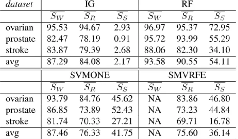
Table 1. Description of mass spectrometry datasets considered. dataset IG RF SW SR SS SW SR SS ovarian 95.53 94.67 2.93 96.97 95.37 72.95 prostate 82.47 78.19 0.91 95.72 93.99 55.29 stroke 83.87 79.39 2.68 88.06 82.30 34.10 avg 87.29 84.08 2.17 93.58 90.55 54.11 SVMONE SMVRFE SW SR SS SW SR SS ovarian 93.79 84.76 45.62 NA 83.86 46.80 prostate 86.85 73.89 52.43 NA 73.23 44.84 stroke 81.74 70.33 27.21 NA 69.71 16.78 avg 87.46 76.33 41.75 NA 75.60 36.14
Table 2. Stability results for the different sta-bility measures. SS is computed on the
fea-ture sets of the best ten feafea-tures proposed by each method.
to a common scale, the absolute values or the squares of the coefficients of the linear hyperplane can be taken to re-flect the importance of the corresponding features, in effect providing a feature weighting. This is actually the assump-tion under which SVMRFE works; alternatively the support vector machine is equivalent to SVMRFE with a single iter-ation, where the ranking of the features is simply based on the absolute values or the squares of the coefficients of the support vector machine. We consider this version of support vector machines as yet another feature selection algorithm and identify it as SVMONE. The implementations of all the algorithms are those found in the WEKA machine learning environment [12].
As already mentioned the stability estimates are cal-culated within each training fold by a nested cross-validation loop and the final results reported are the aver-ages,SW, SR, SS, over the ten external folds.
4 Stability Results
In table 2 we give the stability results forSW,SR, and
SS, i.e., for weightings-scorings, rankings and selected
fea-ture sets, for the four different methods considered. The
values of SS depend on the imposed cardinality of the
fi-nal feature set whileSW andSR are independent of that.
SS was computed on the feature sets of the best ten
fea-tures selected by each method. SVMRFE does not produce a weighting-scoring of features so the computation ofSW
does not make sense in that case. For SVMONE the stabil-ity results are computed on the square values of the coeffi-cients of the linear hyperplane found by the support vector machine.
SW andSRtake into account the complete feature
pref-erences produced by a method, whileSSfocuses on a given
number of top ranked or selected features. Thus the former two provide a global view of stability of feature preferences while the latter focuses to a more precise picture. The latter is usually of greater interest since the feature preferences are in general used to produce a restricted set of features. SW provides a finer grain picture of stability in
compari-son toSRsince it is based on the actuall feature coefficients
produced by a given method while the SR uses the
rank-ing of these coefficients. However this does not mean that the information provided by SW is of greater value than
that provided bySR, but rather the other way around. This
is because again in practise we are more interested in the actual ranks of the features since based on them we will se-lect the final set of features, differences in weights are not necessarily reflected in rank differences. A further disad-vantage ofSW is that since it directly operates on the actual
weights-scores produced by each method its results are not directly comparable among different methods due to possi-ble differences in scales and intervals of the weights-scores, a problem that does not appear when we are working with the ranks. Overall the most important information is de-livered bySS, when we are examining the stability of the
methods for sets of selected features of given cardinality, followed bySR.
This ordering of the three measures in terms of their in-formation content is somehow reflected on the estimated stability performances, table 2. For any methodSW gives
always the highest stability estimate, followed in generally closely by SR. SS is always considerably lower and
de-pends on the number of features that we ask in the final feature set (remember that for the estimates ofSS in table 2
this was set to ten, later we will examine in more detail the behavior ofSS with respect to the cardinality of the final
feature set). In some senseSW andSRprovide overly
op-timistical estimates of feature preference stability (although in no case it can be argued that the values of the different stability measures are comparable). The reason for that can be traced on the fact that they treat all weights or ranks dif-ferences in a uniform manner. Nevertheless difdif-ferences on the highest weighted or ranked features should be penalized more than differences on the lower weighted or ranked fea-tures. A fact that points to the definition and use of more
refined similarity measures that can take into account the level at which a difference appears. These similarity mea-sures would lie conceptually betweenSW, andSR, that give
equal importance to everything, andSS, that only considers
a given number of top ranked features.
We will now examine the stability performance of the four different methods considered. The clear winner is ReliefF that achieves the best performance under all sta-bility measures for the three datasets under consideration. The performance difference is quite astonishing forSS for
which ReliefF scores 72.95%, 55.29% and 34.10% for the ovarian, prostate and stroke datasets respectively. These scores correspond to an average overlap of 8.43, 7.12 and 5.08 features out of the ten contained in the final set of se-lected features, among the different subsets of the training folds1.
Information Gain appears to have a better score than SV-MONE and SVMRFE forSW andSR(remember here that
among the two it isSR that can provide a meaningful
ba-sis for comparison of different methods). However its re-sults are catastrophic when we considerSS, with scores of
2.93%, 0.91% and 2.68% for ovarian, prostate and stroke respectively (an average overlap of 0.56, 0.18, 0.52 features out of the ten, i.e. in average less than one common feature among the different subsets of the training folds!).
Finally the performances of SVMONE and SVMRFE are quite similar in terms of SR a fact that can be easily
explained since the ranking of features provided by SV-MONE can be considered as a less refined version of the ranking provided by SVMRFE with the former being the result of a single execution of the support vector machine algorithm and the latter the result of an iterative execution where each time 10% of the lower ranked features are re-moved. However in terms ofSS SVMONE appears to be
slightly more stable (an average overlap of 6.26, 6.87, 4.27 features out of ten for SVMONE against 6.37, 6.19, 2.87 for SVMRFE). Again the fact that SVMRFE is based on multiple iterations explains its slightly higher instability on the top ten ranked features. When the differences of the coefficients of two features are rather small and a choise is about to be made on which of the two to eliminate different training sets could result in opposite rankings for these two features thus eliminating a different feature each time.
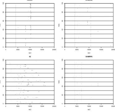
The results of the estimation process ofSS can be very
eloquently visualized providing insight not only on the sta-bility of each individual method, but also clearly indicating which features are considered important by each method. An example of such a visualization for the prostate dataset is given in figure 1 where the cardinality of the final feature set is set to ten. In each of the graphs the x-axis corresponds
1It is easy to compute the actual number of common features when we
know theSSscore and the cardinality of the final feature set simply by the
definition ofSS. 0 5000 10000 15000 20000 0 20 40 60 80 100 IG M/Z folds 0 5000 10000 15000 20000 0 20 40 60 80 100 RELIEF M/Z folds 0 5000 10000 15000 20000 0 20 40 60 80 100 SVMRFE M/Z folds 0 5000 10000 15000 20000 0 20 40 60 80 100 SVMONE M/Z folds
Figure 1. Stability results for the prostate dataset for selected feature sets of cardinality 10.
to the individual features. The y-axis is separated to 10 rows each one corresponding to one of the outer cross-validation folds. Within each row we find 10 rows (not visibly sep-arated) corresponding to each of the inner cross-validation folds of the outer fold. A perfectly stable method, i.e. one that chooses always the same features, would have in its graph as many vertical lines as the cardinality of the final feature set. Each line would correspond to one selected fea-ture. The visualization results are in perfect aggreement with the SS estimates given in table 2. The less stable
method is Information Gain with features sets selected even within the inner folds of a given outer fold being quite dif-ferent (inner folds of a given outer fold share more training instances than the inner folds of two different outer folds). The other three methods are quite stable selecting very often the same features among the different inner folds.
The big differences in the stability estimates ofSRand
SS for Information Gain were puzzling. In order to see
where they could be coming from we took a closer look on the weighting-scorings produced by Information Gain. It turns out that the scorings are zero, i.e. the corresponding features have a zero information gain, for a large number of features. More precisely for ovarian 35.07% of features have an information gain of zero, for prostate this goes up to 85.63%, and for stroke to 91.25%2. On the other hand 2The presence of so many zero information gain features was the result
for ReliefF the corresponding percentages are practically zero, and for SVMONE always less than 3%. When these weightings-scorings are turned into a ranking in order to computeSRthere is a very big number of ties in the
rank-ing of different features (in the case of information gain). The crusial element is how ties are dealt with. Originally we were assigning to all tied features their average rank. This meant that in the case of Information Gain 35.07%, 85.63% and 91.25% of the features, for ovarian, prostate and stroke respectively, had exactly the same rank; more-over these features were concentrated on the low end of the ranking. Due to the presence of a large number of features with equal ranks the final value of theSRestimate was
op-timistically affected for Information Gain, moreover since this was happening on the low rank levels it was completely masking any information about the stability of the rank on the top positions.
To correct for this optimism we have chosen to break ties by assigning randomly the ranks among the tied fea-tures. For example, if below the tenth ranked feature there was a group of 20 features with exactly the same weighting-scoring then each one of them would be assigned a different rank randomly from 11 to 30. This left unaffected theSR
estimates produced for ReliefF, SVMONE, and SVMRFE, since the first two had a very low number of ties, and the latter was naturally producing a rank, but considerably low-ered the stability estimates for Information Gain, with the new estimates being 91.09%, 40.74% and 20.44% for ovar-ian, prostate and stroke respectively, being thus more con-sistent with the picture thatSS is providing. However these
observations still call for a more refined version ofSRthat
would reward similarities and penalize differences more at the top level ranks.
4.1 Stability profiles with
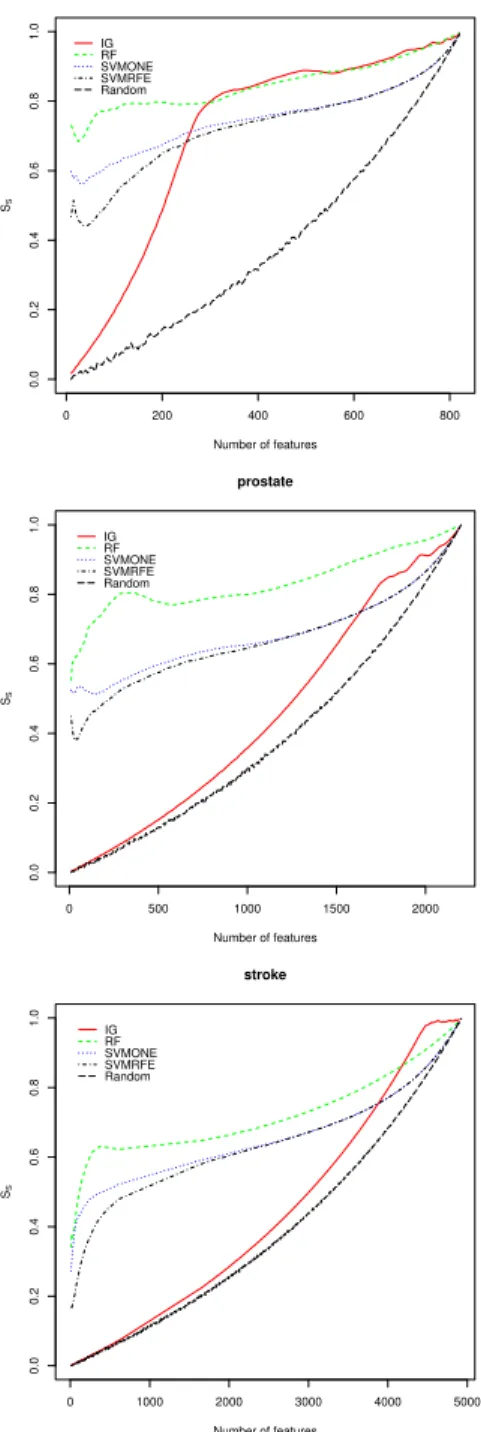
SSIt is clear that the more interesting stability estimation is provided bySS since it focuses only on a small subset
of features, the ones selected by each method, which is ac-tually what interest us when we are performing feature se-lection. To get a more precise picture of the stability per-formance of the different methods with respect toSS we
computed its values for different values of selected features ranging from 10 up to the cardinality of the full feature set with a step a five, figure 2. Moreover we included as a sta-bility baseline a random feature selection that simply out-puts random sets of features of given cardinality.
First remark is that ReliefF clearly dominates all other algorithms for all interesting cardinalities of the final fea-ture sets. Information Gain has a quite bad performance for prostate and stroke, explained by the great number of
of the discretization process that discretized the corresponding features to a single bin.
zero information gain features; actually it has almost the same stability behavior as the random feature selection. In the ovarian dataset it exhibits a sharp increase of stability up to feature sets with around 300 features and then very slowly increases towards one when all features have been included. The ”knot” in this curve actually corresponds to the inclusion of all features, with an information gain dif-ferent than zero, to the final set of selected features. After this point features are actually added randomly. So in some sense it detects the cardinality of the most stable set of fea-tures. The same knot is also observed in the case of RelieF, quite strongly for the stroke and prostate and less for ovar-ian, and for SVMONE and SVMRFE in stroke. We believe that the presence of knots like these mark the inclusion of the most robust-stable features; features included later are added more or less randomly. The knots could be possibly used to determine the optimal cardinality of the most stable feature set, but this is something that needs further investi-gation.
SVMONE has a small advantage over SVMRFE on se-lected feature sets of low cardinality but their performance is indistinguishable for high cardinalities. As we move to higher cardinalities both methods add low ranked features, which should more or less the same for both methods since for SVMRFE these are determined on the earliest iterations of the algorithm, being thus closely in behavior to the single run of SVMONE. Moving to lower cardinalities the insta-bility of SVMRFE increases due to the already mentioned fact that small differences in the coefficients can inverse the rank and thus remove different features. The difference in instability between SVMONE and SVMRFE increases as we move to lower cardinalities beacause there the final fea-ture sets of SVMRFE are determined in the last iterations of the support vector machine algorithm.
5 Stability and Classification Performance
A feature selection algorithm, (FSA for brevity), alone can provide an indication of which features are informative for classification but it cannot provide an estimate of the discriminatory information of these features, since it does not construct classification models whose error could be es-timated. In the same manner stability results cannot provide the sole basis on which to select an appropriate FSA; nev-ertheless they can support the selection of an FSA when the latter is coupled with a classification algorithm, (CA for brevity), and enhance the confidence of the users on the analysis results (provided that the FSA is found to be sta-ble). The final selection can be based on a combined evalu-ation of stability and classificevalu-ation performance.The simplest scenario goes as follows, couple a given CA with a number of FSAs and estimate the classification performance and the stability of the FSA using the process
0 1000 2000 3000 4000 5000 0.0 0.2 0.4 0.6 0.8 1.0 stroke Number of features SS IG RF SVMONE SVMRFE Random 0 500 1000 1500 2000 0.0 0.2 0.4 0.6 0.8 1.0 prostate Number of features SS IG RF SVMONE SVMRFE Random 0 200 400 600 800 0.0 0.2 0.4 0.6 0.8 1.0 ovarian Number of features SS IG RF SVMONE SVMRFE Random
Figure 2.SS plots for varying cardinalities of
the final feature set.
described earlier. Then calculate the statistical significance of error differences. Among the combinations of the CA and FSAs that were found to be better than all the others choose the combination that contains the most stable FSA.
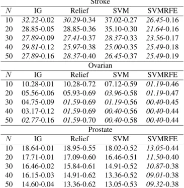
To demonstrate the above idea we selected as classifica-tion algorithm the linear SVM with the complexity param-eter set to 0.5. We performed a series of experiments in which each FSA was paired with the CA. In each experi-ment we fixed the number of selected features to N. We rangedN from ten to 50 with a step of ten. For a givenN the four pairs of FSA-CA were compared with respect to their classification error and the stability of the FSA. Sta-tistical significance of error differences is computed by Mc-Nemar’s test of significance (sig. level=0.05). The complete results are given in table 3. Each row of that table gives the classification errors of a FSA-CA pair followed by the sta-bility estimate,SS, of the FSA. The errors of the FSA-CA
pairs that get the top positions, for a givenN, without being significantly different between them are typed initalics.
Applying the selection scenario mentioned above we see that for stroke and ovarian and for different values of N there are several FSA-CA pairs that are indistinguishable in terms of classification error. Consider the stroke dataset with N = 10; Information Gain, ReliefF and SVMRFE
have similar classification performance. In this case we can also consider their stability. ReliefF is by far the most sta-ble with anSS value that is double of that of SVMRFE and
more than an order of magnitude greater than that of Infor-mation Gain. Obviously the advantage of selecting the most stable FSA is that we have much more confidence on the features. Moreover coupling the results with a visual repre-sentation of stability as the one given in figure 1 provides a clear picture of the important features and how robust they are to perturbations of the training set.
One question that arises from the above results is: how is it possible for a FSA to be very unstable and still when coupled with a CA to produce good results. This was ac-tually the case many times with SVMRFE. For example in the stroke dataset andN = 20SVMRFE coupled with the
CA was signigicantly better than the other three FSA-SA paits. Nevertheless itsSS estimate was 0.16 (in feature sets
of cardinality 20 this corresponds to an average of 5.5 com-mon features). One possible answer to that is redundancy. Among the initial full feature set there are possibly many different subsets of cardinality 20 on which classification models can be constructed that can accurately predict the target concept3. Cases like that, i.e., instability coupled with high classification performance, can be simply an indication of redundancy within the full feature set. This also means that the feature selection algorithm under examination does not have a robust way to tackle redundancy.
3This is true for the mass-spectrometry applications due to the nature
6 Conclusions and Future Work
To the best of our knowledge this is the first time that a framework that measures the stability of feature selection algorithms is proposed. We defined the stability of feature selection algorithms as the sensitivity of the ”feature pref-erences” that they produce to training set perturbations. We examined three different stability measures and proposed a resampling technique to empirically estimate them. The most interesting one was based on SS a measure of the
overlap of two feature sets. We exploited the framework to investigate the stability of some well known feature selec-tion algorithms on three datasets coming from the domain of proteomics and gained some interesting insights. Sta-bility can be also used to support the selection of a feature selection algorithm.
We believe that the notion of stability is central in real world application where the goal is to determine the most important features. If these features are consistent among models created from different traning data the confidence of the users on the analysis results highly increases. The results of the empirical estimation of stability can be ele-gantly visualized and provide a clear picture of the relevant features, their robustnes to different training sets, and the stability of the feature selection algorithm.
Future work includes the examination of stability of more algorithms on a bigger and more diverse set of prob-lems; refining the SR stability measure in order to reflect
better large differences on the top ranked features; aggre-gating the different feature sets produced from subsamples of a given training set in what can be viewed as the analogue of ensemble learning and model combination for feature se-lection; finally we would like to examine the possibility of using the stability profiles to select the appropriate number of features (the knots in the stability graphs).
References
[1] P. Domingos. A unified bias-variance decomposition and
its applications. In P. Langley, editor,Proceedings of the
Seventeenth International Conference on Machine
Learn-ing, pages 231–238. Morgan Kaufmann, 2000.
[2] R. Duda, P. Hart, and D. Stork. Pattern Classification and
Scene Analysis. John Willey and Sons, 2001.
[3] U. Fayyad and K. Irani. Multi–interval discretization of con-tinuous attributes as preprocessing for classification
learn-ing. In R. Bajcsy, editor, Proceedings of the 13th
Inter-national Joint Conference on Artificial Intelligence, pages 1022–1027. Morgan Kaufmann, 1993.
[4] S. Geman, E. Bienenstock, and R. Doursat. Neural networks
and the bias/variance dilemma. Neural Computation, 4:1–
58, 1992.
[5] I. Guyon, J. Weston, S. Barnhill, and V. Vapnik. Gene selec-tion for cancer classificaselec-tion using support vector machines. Machine Learning, 46(1–3):389–422, 2002. Stroke N IG Relief SVM SVMRFE 10 32.22-0.02 30.29-0.34 37.02-0.27 26.45-0.16 20 28.85-0.05 28.85-0.36 35.10-0.30 21.64-0.16 30 27.89-0.09 27.41-0.37 28.37-0.33 23.56-0.17 40 29.81-0.12 25.97-0.38 25.00-0.35 25.49-0.18 50 27.89-0.16 28.37-0.40 26.45-0.37 25.49-0.19 Ovarian N IG Relief SVM SVMRFE 10 10.28-0.01 10.28-0.72 07.12-0.59 01.19-0.46 20 05.56-0.06 05.93-0.69 03.96-0.58 01.19-0.47 30 04.75-0.09 01.59-0.69 01.19-0.56 00.40-0.45 40 03.17-0.12 01.59-0.69 00.40-0.56 00.40-0.44 50 02.77-0.16 01.59-0.70 00.40-0.58 00.40-0.44 Prostate N IG Relief SVM SVMRFE 10 18.64-0.01 18.95-0.55 18.02-0.52 13.05-0.44 20 17.71-0.01 17.09-0.60 16.46-0.51 11.50-0.40 30 16.46-0.02 15.84-0.61 14.91-0.52 10.87-0.38 40 16.15-0.03 14.91-0.62 13.36-0.52 09.01-0.38 50 14.60-0.04 13.36-0.62 13.05-0.53 09.32-0.38
Table 3. Classification error estimations cou-pled with SS stability estimation of the
fea-ture selection method. N is the number of
selected features.
[6] A. Kalousis, J. Prados, E. Rexhepaj, and M. Hilario. Feature extraction from mass spectra for classification. 2005. Sub-mitted to 6th European Conference on Principles and Prac-tice of Knowledge Discovery in Databases.
[7] E. Petricoin, A. Ardekani, B. Hitt, P. Levine, V. Fusaro, S. Steinberg, G. Mills, C. Simone, D. Fishman, E. Kohn, and L. Liotta. Use of proteomic patterns in serum to identify
ovarian cancer.The Lancet, 395:572–577, 2002.
[8] E. Petricoin, D. Ornstein, C. Paweletz, A. Ardekani, P. Hackett, B. Hitt, A. Velassco, C. Trucco, L. Wiegand, K. Wood, C. Simone, P. Levine, W. Marston Linehan, M. Emmert-Buck, S. Steinberg, E. Kohn, and L. Liotta. Serum proteomic patterns for detection of prostate cancer. Journal of the NCI, 94(20), 2002.
[9] J. Prados, A. Kalousis, J.-C. Sanchez, L. Allard, O. Car-rette, and M. Hilario. Mining mass spectra for diagnosis
and biomarker discovery of cerebral accidents.Proteomics,
4(8):2320–2332, 2004.
[10] M. Robnik-Sikonja and I. Kononenko. Theoretical and
em-pirical analysis of relieff and rrelieff. Machine Learning,
53(1–2):23–69, 2003.
[11] P. Turney. Technical note: Bias and the quantification of
stability.Machine Learning, 20:23–33, 1995.
[12] I. Witten and E. Frank. Data Mining: Practical Machine
Learning Tools and Techniques with Java Implementations. Morgan Kaufmann, 1999.