Munich Personal RePEc Archive
Periodic autoregressive conditional
duration
Aknouche, Abdelhakim and Almohaimeed, Bader and
Dimitrakopoulos, Stefanos
University of Science and Technology Houari Boumediene, Qassim
University, Leeds University
8 July 2020
Online at
https://mpra.ub.uni-muenchen.de/101696/
Periodic autoregressive conditional duration
Abdelhakim Aknouche
*, Bader Almohaimeed
**, and Stefanos
Dimitrakopoulos
1****Department of Mathematics, College of Science, Qassim University (Saudi Arabia) & Faculty of
Mathematics, University of Science and Technology Houari Boumediene (Algeria)
**Department of Mathematics, College of Science, Qassim University, Saudi Arabia.
***Division of Economics, Leeds University, UK
Abstract
We propose an autoregressive conditional duration (ACD) model with periodic time-varying parameters and multiplicative error form. We name this model periodic autore-gressive conditional duration (PACD). First, we study the stability properties and the moment structures of it. Second, we estimate the model parameters, using (profile and two-stage) Gamma quasi-maximum likelihood estimates (QMLEs), the asymptotic prop-erties of which are examined under general regularity conditions. Our estimation method encompasses the exponential QMLE, as a particular case. The proposed methodology is illustrated with simulated data and two empirical applications on forecasting Bitcoin trad-ing volume and realized volatility. We found that the PACD produces better in-sample and out-of-sample forecasts than the standard ACD.
Keywords: Positive time series, autoregressive conditional duration, periodic time-varying models, multiplicative error models, exponential QMLE, two-stage Gamma QMLE.
1
Introduction
Recent research in time series analysis tends to avoid transforming original data prior to mod-eling and prefers to represent them directly through models that take into account the actual support of their distributions. Such an approach parallels to that of generalized linear models
(GLM) for independent data (McCullag and Nelder, 1989). In this way, numerous time se-ries models with “specific values” have, recently, received great interest, such as integer-valued models, including count and binary specifications, and positive-valued models.
A well-known model for positive-valued time series data is the autoregressive conditional
duration (ACD), introduced by Engel and Russell (1998). Originally designed to model
du-rations between financial events in high-frequency microstructure markets, the ACD model is also useful for modeling a broad range of data, such as regularly-spaced return range series (Chou, 2005), daily realized volatility (Lanne, 2006; Zheng et al, 2015; Aknouche and Francq, 2019) and trading volume (Li, 2019; Aknouche and Francq, 2020). Various generalizations of the ACD model have been proposed to take into account additional facts of positive time series data (Pacurar, 2008; Hautsch, 2012; Bhogal and Variyam, 2019).
As in the case of GARCH models, it has been documented that the high persistence observed in empirical studies utilizing the standard ACD specification, is in fact artificial and can be avoided by considering ACD models with time-varying parameters (Diebold, 1986; Andersen and Bollerslev, 1997; Mikosch and Starica, 2004; Hejer and Veltic 2007; Caporin et al, 2017; Gallo and Ortanto, 2018). In this paper, we extend the literature on time-varying ACD models, by proposing an ACD model, the parameters of which are allowed to evolve periodically over time. We name this model periodic autoregressive conditional duration (PACD).
Such a model aims to represent seasonally varying positive-valued series. The observed pro-cess is defined as the product of a unit meanindependent and periodically distributed (henceforth
ipdS) innovation process with the conditional mean of the model having a GARCH-type
spec-ification with periodic time-varying parameters. We first study the stability properties of the PACD model, such as the existence of periodically stationary and ergodic solutions with finite moments or log-moments. Such properties are needed in the estimation stage, which is the second contribution of this paper.
is used, since it is well-adapted to the support of the distribution of the data, and it does not require specifying a distribution for the periodically distributed innovation sequence. However, because of the periodicity of that sequence, the EQMLE may be less efficient than the Gamma QMLE (GQMLE) which, in fact, accounts for the periodicity of the model innovation.
Consequently, we propose a two-stage Gamma QMLE (2S-GQMLE) which i) utilizes the EQMLE (or a profile GQMLE) in the first stage, ii) estimates the variance innovations, and then iii) uses the latter as a by-product in the second stage of the computation of the GQMLE. Consistency and asymptotic normality (CAN) of the proposed QMLEs are established and the relative efficiency of the 2S-GQMLE is studied for some specific conditional distributions.
The PACD can be used to model various seasonal positive-valued phenomena (realized volatility, trading volumes and transaction rates). The day-of-the-week pattern may be present in all these phenomena, which means that each day of the week may have its own distribution (Franses and Paap, 2000; Boynton et al, 2009; Tsiakas, 2006; Charles, 2010). In that sense, a time-invariant ACD model for daily data is just an average model that does not take into account the specificities of the underlying measures across days. Other examples of non-financial intraday series that may be characterized by periodicity are wind power and wind speed series (Ambach and Croonenbroeck, 2015; Ambach and Schmid, 2015; Ziel et al, 2016).
Our empirical applications concern Bitcoin trading volume data and the UN realized volatil-ity. Both series are characterized by the day-of-the-week effect and we show that the PACD produces better in-sample and out-of-sample forecasts than the benchmark ACD.
The rest of this paper is outlined as follows. In Section 2 we define the PACD and some special cases of it, and describe the link/relationship between the PACD and the periodic GARCH of Bollerslev and Ghysels (1996). In Section 3 we derive the stability conditions of our model. In Section 4, various Gamma QMLEs are proposed and their asymptotic properties are studied. In section 5 we conduct a simulation study and in section 6 we present the empirical results from two series (Bitcoin trading volume and UN realized volatility). All the proofs are given in the Appendix. A Supplementary material accompanies this paper.
2
Periodic Autoregressive Conditional Duration model
All random variables and processes in this paper are defined on a probability space (Ω,F, P)
and valued in the set of positive real numbers R+ = (0,∞), which is endowed with the Borel
field B(R+). Let S ≥ 1 be a positive integer called the period, and ωt, αt1, ..., αtq, βt1, ..., βtp
(p, q ∈N={0,1, ...}) be positive real parameters S-periodic over time, i.e. ωt =ωt+kS, αti =
αt+kS,i (i= 1, ..., q) andβtj =βt+kS,j (j = 1, ..., p) for all integerskandt. Let also{ξt, t∈Z}be
a sequence of positive random variables with E(ξt) = 1 for allt, and a finite Var(ξt) = σt2 >0.
Assume that {ξt, t∈Z} is ipdS in the sense that ξt D
=ξt+S for all t, where D
= denotes equality in distribution.
A positive-valued stochastic process {Yt, t ∈Z} is said to be a MEM (multiplicative error
model; Engle, 2002) periodicautoregressive conditional durationwith orderspandq(henceforth PACD(p, q)) if Yt is given for all t∈Z by
Yt =ψtξt (2.1a) and ψt=ωt+ q X i=1 αtiYt−i+ p X j=1 βtjψt−j (2.1b)
where the innovation term ξt is independent of ψt−j for all j ≥ 1. To ensure the almost sure
(a.s.) positivity of ψt, it is assumed that ωt >0, αti ≥ 0, and βtj ≥ 0, for all t ∈ Z, i= 1, .., q
and j = 1, ..., p. To emphasize the periodicity of the model, let t = nS +v for n ∈ Z and
1≤v ≤S. Then, equation (2.1b) can be written as follows
ψv+nS =ωv+ q X i=1 αviYv−i+nS + p X j=1 βvjψv−j+nS, n∈Z, 1≤v ≤S,
where by season or channel v (1 ≤ v ≤ S) we denote the set {..., v−S, v, v+S, v+ 2S, ...}
with corresponding parameters ωv, αvi, βvi and σv2 = V ar(ξv+nS). Let Ft be the σ-Algebra
generated by {Yt−i, i≥0}. The conditional mean and conditional variance of the model (2.1)
are given respectively by
and
V ar(Yt|Ft−1) = σ2tψ
2
t. (2.2b)
The PACD model, thus, follows the quadratic variance-to-mean relationship (i.e. the condi-tional variance is proporcondi-tional to the squared condicondi-tional mean), where σ2
t >0 is the variance
of ξt and is S-periodic by construction (from the ipdS property of the innovation sequence {ξt, t∈Z}). The specification (2.1) is a multiplicative error model (MEM) in the sense of
Engle (2002), but the conditional mean equation (2.1b) has rather periodic time-varying coef-ficients. For S = 1, model (2.1) reduces to the standard autoregressive conditional duration (ACD in short) of Engel and Russell (1998). No specification for the distribution of {ξt, t∈Z}
is imposed apart the semiparametric quadratic variance-to-mean function (2.2b). However, a useful family of conditional distributions satisfying (2.2b) is the Gamma distribution with shape
1 σ2 t and scale 1 σ2 tψt, that is Yt|Ft−1 ∼Γ 1 σ2 t, 1 σ2 tψt , (2.3)
where ψt satisfies (2.1b). In the latter case, the innovation term ξt in (2.1) will be marginally
Gamma distributed ξt∼Γ 1 σ2 t, 1 σ2 t , (2.4)
and the process defined by (2.3) is called Gamma PACD(p, q). A notable particular case of model (2.3) appears when the variance σ2
t ≡ 1 is constant, so ξt ∼ Γ (1,1), which corresponds
to theexponential PACD. As in the time-invariant case, the periodic ACD model can be seen as a squared periodic GARCH (PGARCH) model as proposed by Ghysels and Bollerslev (1996). Indeed, consider the following real-valued PGARCH(p, q) process given by
Xt= p htηt (2.5a) and ht=ωt+ q X i=1 αtiXt2−i+ p X j=1 βtjht−j (2.5b)
where {ηt, t∈Z} is an ipdS sequence with mean zero and unit variance, and the parameters
ωt, αti and βtj are defined as above. It is clear that the squared PGARCH process defined by
let {Yt, t∈Z} be a PACD model given by (2.1), and assume {zt, t∈Z} is an independent
and identically distributed (iid) sequence uniformly distributed in {−1,1} (see also Francq and Zakoian, 2019 for the non-periodic case S = 1). Assume {zt, t ∈Z} and {ξt, t∈Z} are
independent and define the process {Xt, t∈Z} by
Xt =zt
p
Yt=
p
htηt
where ht=ψt satisfies (2.5b) and ηt =zt√ξt is a term of an ipdS sequence. Hence {Xt, t∈Z}
is a PGARCH model in the sense of (2.5). Note finally that a PACD model admits a weak periodic ARMA (PARMA) (Lund and Basawa, 2000; Francq etal, 2011). SettingYt=ψt+εt,
the process{Yt, t∈Z} may be written in the following PARMA
Yt=ωt+ max(Xp,q) i=1 (αti+βtj)Yt−i+εt− p X j=1 βtjεt−j where εt=Yt−E(Yt|Ft−1) =ψt(ξt−1) (2.6)
is a zero-mean term of a martingale difference sequence with a finite periodic varianceE(ε2
t) =
E(ψ2
t)E(ξt−1)2 =E(ψt2)σ2t.
A more general PACD, which is not necessarily MEM is defined through a conditional distribution of the form
Yt|Ft−1 ∼Fψt (2.7)
whereFψ is a cumulative probability distribution (with positive support) with meanψ, andψt
is given by (2.1b).
3
Periodic ergodicity and finite moment conditions
We now give necessary and/or sufficient conditions for model (2.1) to be strictly periodically stationary andperiodically ergodic. Such properties are recalled in the Supplementary material. We also consider conditions for the existence of finite moments. Combining (2.1a) and (2.1b)
we obtain the following stochastic recurrence equation (SRE)
Yt=AtYt−1+Bt (3.1)
driven by the ipdS sequence {(At, Bt), t∈Z}, where Yt = (Yt, ..., Yt−q+1, ψt, ..., ψt−p+1)′, Bt =
ωtξt,0(q−1)×1, ωt,0(p−1)×1 ′ , and At= αt1ξt · · · αt,q−1ξt αtqξt βt1ξt · · · βt,p−1ξt βtpξt 1 · · · 0 0 0 · · · 0 0 ... . .. ... ... ... . .. ... ... 0 · · · 1 0 0 · · · 0 0 αt1 · · · αt,q−1 αtq βt1 · · · βt,p−1 βtp 0 · · · 0 0 1 · · · 0 0 ... . .. ... ... ... . .. ... ... 0 · · · 0 0 0 · · · 1 0 ,
0m×n being the null matrix of dimension m×n. Let
γS = inf
1
nElogkAnS...A2A1k, n≥1
be the top Lyapunov exponent associated with the ipdS-driven SRE (3.1) (Aknouche et al,
2020). Let also βt= βt1 · · · βt,p−1 βtp 1 · · · 0 0 ... ... ... ... 0 · · · 1 0 ,
and denote by ρ(A) the spectral radius of the squared matrix A, i.e. the maximum modulus of the eigenvalues of A. The following result gives the conditions for equation (3.1) to have a unique strictly periodically stationary and periodically ergodic solution.
Theorem 3.1 i) Assume E(log (ξv)) <∞ for all 1 ≤ v ≤ S. A necessary and sufficient
periodically ergodic solution is that
γS <0. (3.2)
Such a solution is given for all t∈Z by
Yt= ∞ X j=0 j−1 Y i=0 At−iBt−j, (3.3)
where the series in the right hand side of (3.3) converges absolutely almost surely.
ii) If (2.1)admits a strictly periodically stationary solution then
ρ SY−1 v=0 βS−v ! <1. (3.4)
In the special case where p = q = 1, the periodic stationarity condition (3.2) is simplified as follows S X v=1 E(log (αvξv−1+βv))<0, while (3.4) reduces to S Q v=1 βv <1.
Conditions for the existence of moments of the P ACD(p, q) process are given as follows.
Theorem 3.2 Assume E(ξv)<∞for all 1≤v ≤S. A sufficient condition for the process
given by (2.1) to be strictly periodically stationary and periodically ergodic with E(Yt)<∞ is
that ρ SY−1 v=0 E(AS−v) ! <1. (3.5)
Some remarks are in order:
- In the case, where S = 1, the conditional mean coefficients are time-invariant, that is
ωtj =ω, αtj =αj andβtj =βj. Therefore, using a similar device by Chen and An (1998), (3.5)
reduces to the following stationarity in mean condition
q X i=1 αi+ p X j=1 βj <1
as provided by Engle and Russell (1998).
following condition
S Y v=1
(αv +βv)<1. (3.6)
Theorem 3.3 i)Under (3.2) there exists κ >0 such that for all 1≤v ≤S
E(ψvκ)<∞ and E(Y
κ
v )<∞. (3.7)
ii) Let {Yt, t∈Z} be a strictly periodically stationary solution of (2.1) and assume that
E(ξm
v ) (m∈N∗) is finite for all 1≤v ≤S. A sufficient condition for E(Yvm) to be finite (for
all 1≤v ≤S) is that ρ SY−1 v=0 E A⊗m S−v ! <1 (3.8)
where A⊗m is the Kronecker product: A⊗A⊗ · · · ⊗A with m factors.
In the special case of Gamma PACD with p=q = 1, explicit conditions equivalent to (3.8) can be given. These conditions are also necessary for the existence of finite moments.
Proposition 3.1 The Gamma P ACD(1,1) model (2.3) admits a unique nonanticipative
periodically ergodic solution {Yt, t∈Z} such that:
i) E(Yv)<∞ (1≤v ≤S) if and only if (3.6) holds.
ii) E(Y2
v)<∞ ( 1≤v ≤S) if and only if E(ξv2)<∞ (1≤v ≤S), (3.6) and
S Y v=1 α2vE ξv2−1+ 2αvβv +βv2 <1. (3.9) iii) E(Y3
v)<∞ (1≤v ≤S) if and only if E(ξv3)<∞ ( 1 ≤v ≤S), (3.6), (3.9) and
S Y v=1 E ξv3−1α3v+ 3 σv2−1+ 1α2vβv+ 3αvβv2+β 3 v <1. (3.10) iv) E(Y4 v) < ∞ (1≤v ≤S) if and only if E(ξv4) < ∞ ( 1 ≤v ≤S), (3.6), (3.9), (3.10)
and the following hold
S Y v=1 E ξv4−1 α4v + 4 1 +σ2v−1 1 + 2σ2v−1 α3vβv+ 6 1 +σv2−1 α2vβv2+ 4αvβv3+βv4 <1. (3.11) For the particular exponential PACD(1,1) model, Yt|Ft−1 ∼ Γ
1, 1
ψt
Proposition 3.1 the moments E(ξ2v), E(ξv3) and E(ξv4) by 1, 6 and 24 respectively, and σv2
by 1 for all 1≤v ≤S.
4
Gamma quasi-maximum likelihood estimates
LetY1, Y2, ..., YT be a series generated from the PACD(p, q) model, which we can rewrite in the
following form YnS+v =ψnS+vξnS+v, ψnS+v =ψnS+v(θ0) = ω0v+ q P i=1 α0 viYnS+v−i+ p P j=1 β0 vjψnS+v−j, 1≤v ≤S, n∈Z (4.1)
where the true parameter θ0 = (θ01′, θ20′, ..., θS0′)′ with θv0 = (ωv0, α0v1, ..., αvq0 , βv01, ..., βvp0 )′ (1≤v ≤
S) belongs to a parameter space Θ ⊂ (0,∞)×[0,∞)(p+q)S. The true innovation variance parameter σ2
0 = (σ201, ..., σ20S)′ withσ02v =V ar(ξnS+v) (1≤v ≤S) also belongs to a parametric
space ∆ ⊂ RS
+. The sample size T = N S (N ≥ 1) is assumed without loss of generality a multiple ofS. Given initial valuesY0, ..., Y1−q,ψe0, ...,ψe1−p and a generic parameterθ∈Θ define
e ψnS+v(θ) = ωv+ q X i=1 αviYnS+v−i+ p X j=1 βvjψenS+v−j(θ), 1≤v ≤S, n≥0, (4.2a)
as an observable proxy for ψnS+v(θ). The latter is defined as a periodically stationary solution
of the following generic model (θ ∈Θ)
ψnS+v(θ) =ωv+ q X i=1 αviYnS+v−i+ p X j=1 βvjψnS+v−j(θ), 1≤v ≤S, n∈Z. (4.2b)
4.1
Exponential and profile Gamma QMLEs
The true conditional distribution of (4.1) is unknown due to the unpecification of the law of
ξv (1 ≤ v ≤S). Thus, a quasi-maximum likelihood estimate (QMLE) which does not require
any precise knowledge of the conditional distribution is suitable for estimating the parameter
θ0 involved in the conditional mean. Among many possible QMLEs, the one computed on the basis of the exponential distribution (EQMLE in short) is especially useful for positive duration data because it reduces to the maximum likelihood estimate when ξv is exponentially
distributed (Aknouche and Francq, 2020). A more general QMLE, which can be more efficient than the EQMLE in the periodic time-varying innovation context is the one computed on the basis of the Gamma distribution with arbitrary fixed variance parameters. Let (σ2
t)t be fixed
known positive numbers, S-periodic over t, i.e. σ2
v+kS = σv2, for all k ∈ {0, ..., N −1}. The
profile Gamma likelihood associated with σ2 = (σ2
1, ..., σS2)′ >0 is given, ignoring constants, by
e LT (θ) =T1 T X t=1 elt(θ), (4.3a) elt(θ) =σ12 t Yt e ψt(θ)+ log e ψt(θ) , t≥1. (4.3b)
The profile Gamma QMLE (GQMLE) θbG of θ0 is, then, the minimizer ofLeT (θ) over Θ, b
θG = arg min
θ∈ΘLeT (θ) . (4.4)
When σ2 = (1, ...,1)′, the GQMLE defined by (4.4) reduces to the EQMLE and is denoted
byθbE (Aknouche and Francq, 2020).
LetγS(A0) be the top Lyapunov exponent associated with (A0
t, t∈Z) where the matrixA0t
is just At defined in (3.1) with θ0 in place of θ. To establish the strong consistency of θbG we
need to the following assumptions.
A1 γS(A0)<0 and ∀θ ∈Θ, ρ S−1 Q v=0 βS−v <1. A2 θ0 ∈Θ and Θ is compact. A3 The polynomials α0 v(z) = q P i=1 α0 vizi and βv0(z) = 1− p P j=1 β0
vjzj have no common root,
α0
v(1)6= 0, and αvq0 +βvp0 6= 0 for all 1≤v ≤S.
A4 ξv is non-degenerate for all 1≤v ≤S.
As seen in Section 3,γS(A0)<0 inA1ensures periodic stationarity and periodic ergodicity of the PACD model (4.1). The condition ρ
S−1 Q v=0
βS−v
< 1 is imposed for the invertibility of equation (4.2b) for any θ∈Θ. The compactness assumption A2 is standard while A3 and A4
are made to guarantee the identifiability of the model.
Theorem 4.1 Let θbG
be a sequence of EQMLEs defined by (4.3). Under A1-A4,
b
Turn now to the asymptotic normality property of bθG. The following assumptions are to be
considered.
A5 θ0 belongs to the interior of Θ.
A6 The matrices I θ0, σ2 = S X v=1 σ2 0v σ4 v E 1 ψ2 v(θ0) ∂ψv(θ0) ∂θ ∂ψv(θ0) ∂θ′ , J θ0, σ2 = S X v=1 1 σ2 vE 1 ψ2 v(θ0) ∂ψv(θ0) ∂θ ∂ψv(θ0) ∂θ′ (4.5)
are finite, and J(θ0, σ2) is nonsingular for all σ2 >0.
Theorem 4.2 Under A1-A6 we have
√ NθbG−θ0 D →N (0,Σ) asN → ∞ for all σ2 >0 (4.6a) where Σ =J θ0, σ2− 1 I θ0, σ2J θ0, σ2− 1 (4.6b)
is block-diagonal and →D stands for convergence in distribution.
Remark 4.1
i) When σ2 = (1, ...,1)′ := 1, the EQMLE has a covariance matrix in a ”sandwich” form
and is, in general, not asymptotically efficient unlessσ2
0 =1and the conditional distribution is exponential.
ii) For the special exponential PACD(p, q) model corresponding to V ar(ξv) = 1 for all
1≤ v ≤ S, if we set σ2 =1 then J(θ
0,1) =I(θ0,1) and the asymptotic covariance matrix of the EQMLE reduces to Σ =J(θ0,1)−1. The EQMLE is thus asymptotically efficient.
iii) If ξv has a constant variance, i.e. σ02v =V ar(ξv) =σ20 for all 1 ≤v ≤S, then it suffices to take σ2 = (1, ...,1)′ and apply the EQMLE. We would have I(θ
0,1) = σ02J(θ0,1) and the covariance matrix would be equal to Σ = σ2
0J(θ0,1)−1. In this case, the EQMLE is the best QMLE among all QMLEs belonging to the linear exponential family.
iv) For the non-periodic ACD corresponding to S= 1 and then σ2
0v =σ02 for all 1≤v ≤S, it is natural to take σ2
v = σ2 for all 1≤ v ≤ S. In this case, the profile likelihood (4.3) would
be given by Let(θ) = σ12T1 T P t=1 Yt e ψt(θ) + log e ψt(θ)
and the resulting GQMLE then reduces to
maximizing T1 T P t=1 Yt e ψt(θ) + log e ψt(θ)
is why, in general, the EQMLE is the most used QMLE for non-periodic ACD even when the latter is strictly (conditionally) Gamma distributed.
v) When the profile varianceσ2coincides with the true varianceσ2
0we would haveJ(θ0, σ02) =
I(θ0, σ02) and Σ =J(θ0, σ20)− 1
, where the GQMLE is the most efficient among all QMLEs be-longing to the exponential family. As σ2
0 is generally unknown, a crucial step is to get a consistent estimate bσ2
0 and construct with it an estimated (profile) log-likelihood from which a new Gamma QMLE, called the two-stage Gamma QMLE (2S-GQMLE), is computed. The resulting estimate would have the aforementioned efficiency property.
vi) Theorem 4.1 and 4.2 also hold for the non-MEM PACD (2.7). It suffices to replace the assumptions A1-A4 by the following:
A1’ The process {Yt, t∈Z} is strictly periodically stationary and periodically ergodic.
A2’E Yt1+ǫ
<∞ for someǫ >0.
A3’ψt(θ) =ψt(θ0) a.s. ⇒θ =θ0.
4.2
Estimating the innovation variances
To estimate the unknown variances σ20 under the MEM constraint recall (2.1)-(2.2) and let
ut = (Yt−ψt)2−V ar(Yt|Ft−1) =ψ2t (ξt−1)2−σ02t . Then, (Yt−ψt)2 ψ2 t =σ 2 0t+vt (4.7a) where vt = ψut2 t = (ξt−1) 2 − σ2
0t. The sequence (vt) is thus zero-mean iid with variance
E (ξt−1)2−σ20t
2
, which is finite under the following assumption.
A7 E(ξv4)<∞for all v = 1, ..., S.
Since ψt=ψt(θ0) depends on the unknown parameter θ0, the regressand in (4.7a) is unob-servable. If we replace θ0 by a consistent estimate, say the GQMLE in (4.4), then we get the following approximate regression but with observable regressand
(Yt−ψbt) 2 b ψ2 t =σ20t+bvt, (4.7b)
where ψbt=ψt
b
θG
. From (4.7b) a feasible OLS estimate (OLSE) ofσ2
0 is given by b σ2v = 1 N NX−1 n=0 (Yv+nS−ψbv+nS) 2 b ψ2 v+nS , for all v = 1, ..., S. (4.8)
The following result shows that the OLSE σb2
v (1≤v ≤S) is consistent and asymptotically
Gaussian.
Theorem 4.3 Under A1-A4
b
σ2
v →σ02v a.s. asN → ∞, for all v = 1, ..., S. (4.9a)
If in addition A7 holds then for all v = 1, ..., S
√ N bσv2−σ20v D →N (0,Λv) as N → ∞ (4.9b) where Λv =E (ξv −1)2−σ02v 2 .
A consistent estimate of the limiting variance Λv in (4.9b) is given by
b Λv = N12 NX−1 n=0 b ξv+nS−1 2 −bσv2 2 , v = 1, ..., S, (4.10) where ξbv+nS = Yv+nS b
ψv+nS is the residual of model (2.1). With (4.9b) and (4.10), the asymptotic
matrices in (4.5) may also be estimated. A consistent estimate of Σ is
b Σ =Jb−1Ib−1Jb−1 (4.11) where b J = N1 NX−1 n=0 S X v=1 1 σ2 vψv2+nS(θbG) ∂ψψv+nS(θbG) ∂θ ∂ψψv+nS(θbG) ∂θ′ , Ib= 1 N NX−1 n=0 S X v=1 b σ2 v σ4 vψv2+nS(θbG) ∂ψv+nS(bθG) ∂θ ∂ψv+nS(θbG) ∂θ′ .
4.3
Two-stage Gamma QMLE
We have seen above that the asymptotic distribution and then the asymptotic efficiency of the profile GQMLE depend on the choice of the profile varianceσ2. To improve the efficiency of the
GQMLE, we can replace in (4.4) the profile variancesσ2 by the OLS estimatesσb2 = (bσ21, ...,bσ2S)′
given by (4.8). The resulting estimate is denoted by 2S-GQMLE and is given by the following steps.
Algorithm 4.1 Two-stage GQMLE
i) Fix an arbitrarily σ2 >0, for example σ2 = (1, ...,1)′.
ii) Get the profile GQMLE θbG from (4.4).
iii) Estimate the variance innovation σ2
0 using bσ2 in (4.8).
iv) Consider the 2S-GQMLE as a solution of the following problem
b θ∗G= arg min θ∈Θ NX−1 n=0 S X v=1 Y v+nS b σ2 vψev+nS(θ) + 1 b σ2 vlogψev+nS(θ) . (4.12)
Consistency of asymptotic normality of bθ∗
G are a by-product of Theorems 4.1-4.2.
Corollary 4.1 Under A1-A4
√
Nθb∗G−θ0
D
→N 0, J θ0, σ2−1 as N → ∞for all σ2 >0.
The latter result shows that whatever the distribution of (ξv)v is, the 2S-GQMLE bθ∗G is
asymptotically the most efficient one among all QMLEs belonging to the linear exponential family (cf. Gourieroux etal, 1984; Wooldridge, 1999). In particular, θb∗
Gin never asymptotically
less efficient than the profile GPQMLEθbG and therefore than the EQMLE bθE.
5
Simulation study
We examine the finite-sample behavior of the Gamma QMLEs, as defined above, using many simulated PACD(1,1) series with sample size T = 2000. We consider two distributions for the innovation ξt in (2.1), namely i) the exponential distribution (ξt ∼ E (1) ≡ Γ (1,1)) so that
Yt|Ft−1 ∼ Γ (1,1/ψt), and ii) the Gamma distribution (ξt ∼ Γ σ0−t2, σ0−t2
) so that Yt|Ft−1 ∼ Γ σ0−t2, σ−0t2/ψt
, whereσ0−v2 (1≤v ≤S).
For these two cases we take S = 5, which is representative of many real daily trading measurements, such as trading volumes and realized volatilities. The true conditional mean parameters, which are reported in Tables 5.1 and 5.2, are chosen so that the PACD model to
be stable in the sense of Section 3, while implying fairly persistent series that are in accordance with the empirical evidence. For each case and for each series we compute the EQMLE and the two-stage GQMLE (2S-GQMLE), using 1000 Monte Carlo replications.
The starting parameter value in the nonlinear optimization routines (4.4) and (4.12) is set to the true value, while the unobservable starting valuesY0 andψ0(θ) of the PACD(1,1) equation are set to the intercept ω0
0. The two-stage GQMLE is calculated, with the EQMLE computed in the first stage.
EQMLE 2S-GQMLE v θ0 v ω0v α0v βv0 σ20v ωv0 α0v βv0 1 True Mean Std 0.5 0.5191 0.3163 0.6 0.5981 0.0709 0.35 0.3484 0.0698 1 0.9817 0.0968 0.5 0.5191 0.3168 0.6 0.5980 0.0710 0.35 0.3484 0.0699 2 True Mean Std 0.9 0.8941 0.3624 0.4 0.4003 0.0723 0.5 0.5039 0.0921 1 0.9917 0.1001 0.9 0.8940 0.3628 0.4 0.4001 0.0723 0.5 0.5040 0.0924 3 True Mean Std 1.5 1.4558 0.4795 0.5 0.5006 0.0784 0.5 0.5063 0.1010 1 0.9837 0.0992 1.5 1.4559 0.4806 0.5 0.5005 0.0783 0.5 0.5063 0.1011 4 True Mean Std 0.45 0.4521 0.4000 0.45 0.4490 0.0635 0.45 0.4453 0.0795 1 0.9859 0.1041 0.45 0.4525 0.4007 0.45 0.4492 0.0636 0.45 0.4452 0.0798 5 True Mean Std 0.7 0.6797 0.3828 0.55 0.5512 0.0726 0.40 0.4051 0.0804 1 0.9792 0.0939 0.7 0.6793 0.3832 0.55 0.5510 0.0728 0.40 0.4053 0.0806 Table 5.1. EQMLE and 2S-GQMLE results for 1000 PACD(1,1) series withn = 2000
generated from the exponential Γ (1,1/ψt) distribution.
Means and standard deviations of the estimates bθE and θb∗G over the 1000 replications are
reported in Table 5.1 for the exponential PACD(1,1) model and in Table 5.2 for the homolog Gamma PACD(1,1) model. It can be observed from Tables 5.1-5.2 that the results are consistent
with asymptotic theory. They are indeed almost identical in the exponential case with a slight superiority of the EQMLE over the 2S-GQMLE (cf. Table 5.1). The two estimates are, in fact, asymptotically efficient in this case but the EQMLE is much simpler to compute. For the Gamma PACD model in Table 5.2, θb∗
G outperforms θbE in terms of bias and variability, as
expected. In all cases, the 2S-GQMLE is the least risky one in the misspecification case.
EQMLE 2S-GQMLE v θ0 v ω0v α0v βv0 σ20v ωv0 α0v βv0 1 True Mean Std 0.2 0.2099 0.1573 0.4 0.4022 0.0408 0.5 0.4991 0.0768 0.5 0.4976 0.0428 0.2 0.2020 0.1550 0.4 0.4012 0.0399 0.5 0.5006 0.0754 2 True Mean Std 0.9 0.8843 0.1462 0.3 0.3045 0.0654 0.6 0.6046 0.0891 0.3 0.2981 0.0240 0.9 0.8934 0.1452 0.3 0.3036 0.0553 0.6 0.6009 0.0798 3 True Mean Std 0.3 0.3341 0.2856 0.5 0.5030 0.1130 0.4 0.3815 0.1240 1.5 1.4729 0.1582 0.3 0.3417 0.2826 0.5 0.5058 0.1100 0.4 0.3777 0.1201 4 True Mean Std 0.4 0.4040 0.2645 0.45 0.4526 0.0702 0.45 0.4534 0.0971 1 0.9809 0.0935 0.4 0.3995 0.2599 0.45 0.4525 0.0681 0.45 0.4541 0.0933 5 True Mean Std 0.5 0.4997 0.2729 0.55 0.5546 0.0921 0.35 0.3494 0.1002 2 1.9424 0.2247 0.5 0.4923 0.2487 0.55 0.5546 0.0834 0.35 0.3533 0.0838 Table 5.2. EQMLE and 2S-GQMLE results for 1000 PACD(1,1) series with T = 2000
generated from the Gamma Γ (1/σ2
0t,1/σ20tψt) distribution.
6
Empirical applications
6.1
Application to Bitcoin trading volume data
In our application, we fit the PACD(1,1) model to the daily Bitcoin trading volume (BTV). The dataset was obtained from the webpage www.blockchain.com. This series spans from July,
Figure 6.1: Daily Bitcoin trading volume (BTV).
3, 2017 to June, 26, 2020, with a total ofT = 1092 = 7×156 observations. Figure 6.1 displays the time series plot of the data.
In the context of Bitcoin prices, Mbanga (2019) found evidence of the presence of the day-of-the-week pattern. Our aim here is to show that the Bitcoin volume data are also characterized by the day-of-the-week effect, which implies a period of S = 7. Such a case is different from the data usually encountered in non-cryptocurrency returns (such as stocks, exchange rates), which are characterized by a periodicity of S = 5, due to the existence of non-trading days at each week (Franses and Paap, 2000; Tsiakas, 2006).
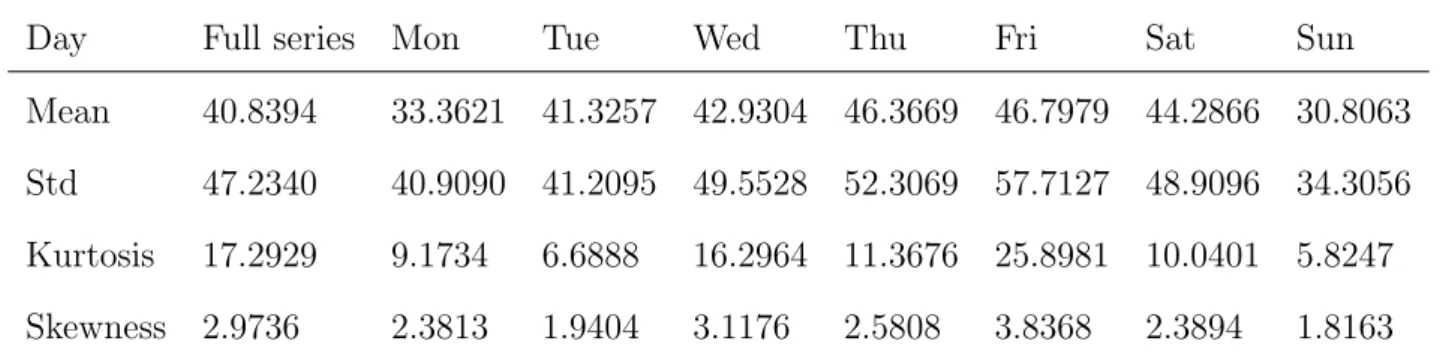
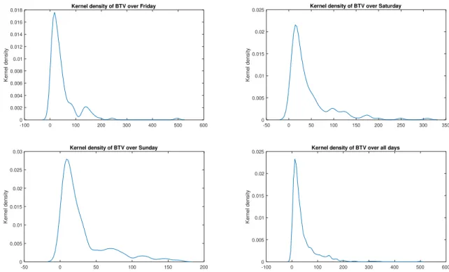
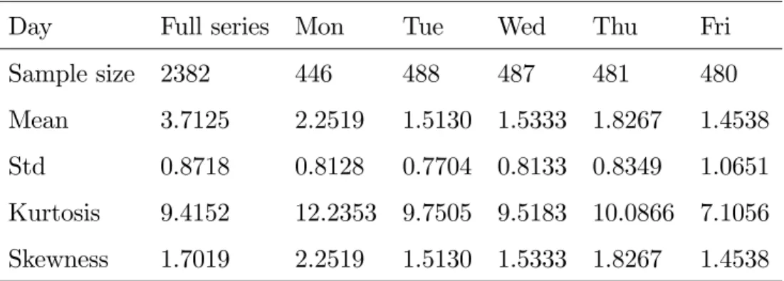
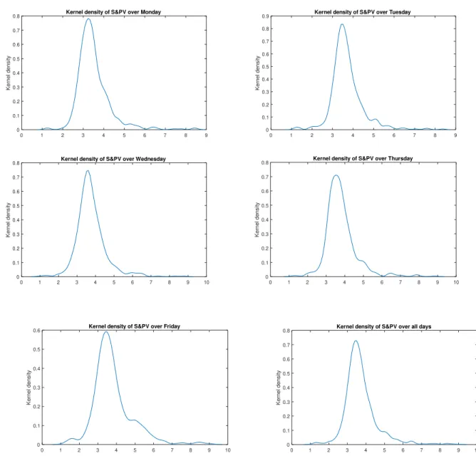
Table 6.1 provides some descriptive statistics for the full sample and for each day of the week separately. The mean of BVT series is clearly different from one day to another. The difference is more pronounced for the Kurtosis and skewness across the days. Also, the estimated kernel densities of the data across the days are visually different (see Supplementary material). In that regard, we suspect that the day-of-the week effect may characterize the Bitcoin trading volume series.
Day Full series Mon Tue Wed Thu Fri Sat Sun Mean 40.8394 33.3621 41.3257 42.9304 46.3669 46.7979 44.2866 30.8063 Std 47.2340 40.9090 41.2095 49.5528 52.3069 57.7127 48.9096 34.3056 Kurtosis 17.2929 9.1734 6.6888 16.2964 11.3676 25.8981 10.0401 5.8247 Skewness 2.9736 2.3813 1.9404 3.1176 2.5808 3.8368 2.3894 1.8163
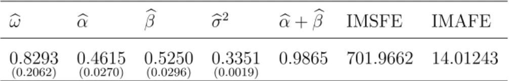
We first estimate a standard ACD(1,1) model (i.e. PACD with S = 1), using the EQMLE as recommended in Remark 4.1, (iv). This model is used as a competitor to our PACD(1,1). The initial parameter values are set to θ(0) = ω(0), α(0), β(0) = (0.1,0.3,0.5) and the starting values of the conditional mean equation are fixed toY0 =ψ0 =ω(0). The estimated parameters and their asymptotic standard errors (ASE) in parentheses, obtained from Theorem 4.2-4.3, are reported in Table 6.2. In particular, the ASE of σb2 is computed from (4.10). The persistence parameter estimate, αb+βb= 0.9865, indicates a strong persistence in the series, as expected.
b
ω αb βb bσ2 αb+βb IMSFE IMAFE 0.8293
(0.2062) 0(0..46150270) 0(0.5250.0296) 0(0.3351.0019) 0.9865 701.9662 14.01243 Table 6.2. EQML estimates for the ACD(1,1); BTV series.
Table 6.2 also displays the in-sample mean square (one-step ahead) forecast error (IMSFE) and the in-sample mean absolute forecast error (IMAFE) given by IMSFE= 1
T T P t=1 (Yt−ψbt)2 and IMAFE= T1 T P t=1 Yt−ψbt
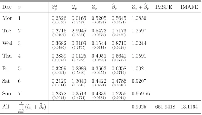
, respectively. Unreported sample autocorrelations of the residu-als consolidate the validity of the estimated ACD(1,1). Since this model does not take into account the day-of-the-week effect, we fit a 7-periodic PACD(1,1) to the BVT series. To this end, we utilize the 2S-GQMLE by starting from the EQMLE in the first stage with the fol-lowing initial parameter values for the optimization routine: ω(0) = (0.6,0.25,0.35,3,2,4,1.5),
α(0) = (0.25,0.15,0.1,0.3,0.3,0.4,0.35) and β(0) = (0.7,0.8,0.85,0.4,0.5,0.2,0.45). These ini-tial values are arbitrary but we checked that the estimates are robust even with other iniini-tial
values. Day v σb2 v ωbv αbv βbv αbv +βbv IMSFE IMAFE Mon 1 0.2526 (0.0050) 0(0..01653537) 0(0.5205.0421) 0(0.5645.0481) 1.0850 Tue 2 0.2716 (0.0102) 2(0..99454361) 0(0.5423.0379) 0(0.7173.0430) 1.2597 Wed 3 0.3682 (0.0180) 0(0..31092705) 0(0.1544.0414) 0(0.8710.0428) 1.0244 Thu 4 0.2839 (0.0075) 0(0..01256255) 0(0.4951.0690) 0(0.5641.0772) 1.0591 Fri 5 0.3299 (0.0092) 0(0..28895360) 0(0.3663.0655) 0(0.6358.0714) 1.0021 Sat 6 0.2129 (0.0014) 1(0..30405645) 0(0.4422.0724) 0(0.4786.0810) 0.9207 Sun 7 0.2372 (0.0043) 0(0..35134721) 0(0.4339.0781) 0(0.2256.0914) 0.659 56 All 7 Q v=1 (αbv +βbv) 0.9025 651.9418 13.1164
Table 6.3. 2S-GQML estimates for the PACD(1,1); BTV series.
The 2S-GQML estimates and their ASEs in parentheses are reported in Table 6.3. We observe that the estimates are quite different across the days. The persistence parameters over the days show locally explosive behaviors except for Saturday and Sunday. However, the whole persistence parameter, Q7v=1(αbv +βbv) = 0.9025 (also called the monodromy estimate) is, as
expected, considerably smaller than the one given by the estimated standard ACD(1,1). All results have been obtained irrespective of any distributional specification of the models.
Note that the ASE of estimates for the PACD are larger than those obtained for the ACD. This is due to the fact that for the PACD the ASEs are computed for lower channel series with sample size T
S = 156. To get the same precision as with the ACD we should consider larger
series with the sample size multiplied at least by 7. Nevertheless, in term of in-sample forecast ability (IMSFE and IMASE), the PACD model outperforms the standard ACD.
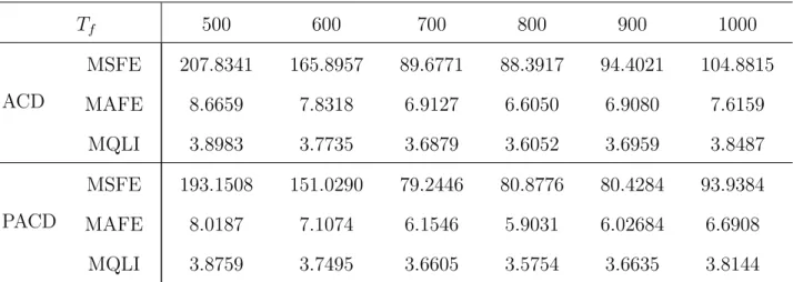
To compare the out-of-sample forecasting performance of the two models, we estimate the two competing models on the basis of the first Tf observations of the series, where 1 < Tf < T.
Then, we compute the one-step ahead forecast on the period (Tf + 1, ..., T) based on
b
We finally calculate for each model the following three criteria: i) the mean square forecast error MSFE= 1 T−Tf T P t=Tf+1
(Yt −ψbt)2, ii) the mean absolute forecast error MAFE =
1 T−Tf T P t=Tf+1 Yt−ψbt
, and iii) the mean QLIKE (cf. Patton, 2011; Aknouche and Francq, 2019) MQLI= T−1T f T P t=Tf+1 (logψbt+ Yψbt t).
Table 6.4 shows these computed values of these criteria for the two models and for various truncated series with sample sizeTf. It can be observed that irrespective of the chosen sample
size, the PACD yields better out-of-sample forecasts with regard to the aforementioned criteria. Overall, the PACD(1,1) outperforms the ACD(1,1), both in terms of in-sample and out-of-sample forecasting power.
Tf 500 600 700 800 900 1000 ACD MSFE MAFE MQLI 207.8341 8.6659 3.8983 165.8957 7.8318 3.7735 89.6771 6.9127 3.6879 88.3917 6.6050 3.6052 94.4021 6.9080 3.6959 104.8815 7.6159 3.8487 PACD MSFE MAFE MQLI 193.1508 8.0187 3.8759 151.0290 7.1074 3.7495 79.2446 6.1546 3.6605 80.8776 5.9031 3.5754 80.4284 6.02684 3.6635 93.9384 6.6908 3.8144 Table 6.4. Out-of-sample forecasting performance of the PACD and ACD; BVT series.
6.2
Application to the UN realized volatility
The second dataset is the daily UN realized volatility (RV) that covers the sample period from January 04, 1999 to December, 31, 2008 with a total of T = 2489 observations. The plot of the index series is displayed in Figure 6.2.
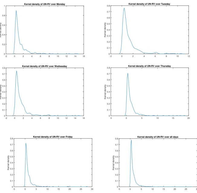
Table 6.5 reports some descriptive statistics concerning the whole series and the subseries corresponding to the five trading days. It can be easily seen that these statistics strongly indicate that the distributions of realized volatility are significantly different across the trading days. This is also confirmed by the estimated kernel density of each trading day (Supplementary
Figure 6.2: Daily UN realized volatility UN (UN-RV).
material). These facts suggests using a 5-periodic PACD(1,1) model for these data.
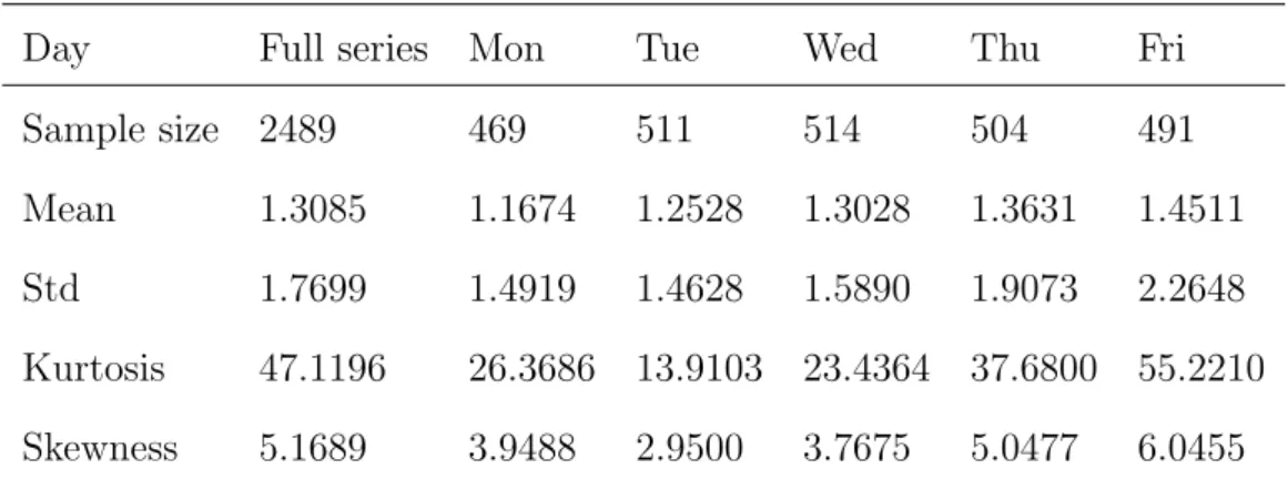
Day Full series Mon Tue Wed Thu Fri Sample size 2489 469 511 514 504 491 Mean 1.3085 1.1674 1.2528 1.3028 1.3631 1.4511 Std 1.7699 1.4919 1.4628 1.5890 1.9073 2.2648 Kurtosis 47.1196 26.3686 13.9103 23.4364 37.6800 55.2210 Skewness 5.1689 3.9488 2.9500 3.7675 5.0477 6.0455
Table 6.5. Day-of-the-week pattern in the UN-RV series.
As a reference model, we first estimate a standard ACD(1,1) for the data. Table 6.6 shows the EQML estimates and their asymptotic standard errors in parenthesis. The results signal a high persistence near to instability.
b
ω αb βb bσ2 αb+βb IMSFE IMAFE 0.0109
(0.0031) 0(0..28490157) 0(0..70840162) 0(0.2841.0005) 0.9933 1.1122 0.4842 Table 6.6. EQML estimates for the ACD(1,1); UN-RV series.
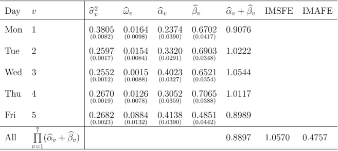
Table 6.7 displays the 2S-GQML estimates of the PACD(1,1) based on the UN-RV series. These estimates are quite different across the days and are all significant. Also, the persistence parameter, given byQ7v=1(αbv+βbv) = 0.8897, is significantly smaller than that obtained from the
the ACD. The ASEs of the estimates for the PACD are smaller than in the first application, since the series here is quite longer. Moreover, the PACD model outperforms the standard
ACD, according to the IMSFE and IMASE criteria. Day v σb2 v ωbv αbv βbv αbv +βbv IMSFE IMAFE Mon 1 0.3805 (0.0082) 0(0..01640098) 0(0.2374.0390) 0(0.6702.0417) 0.9076 Tue 2 0.2597 (0.0017) 0(0..01540084) 0(0.3320.0291) 0(0.6903.0348) 1.0222 Wed 3 0.2552 (0.0012) 0(0..00150088) 0(0.4023.0327) 0(0.6521.0354) 1.0544 Thu 4 0.2670 (0.0019) 0(0..01260078) 0(0.3052.0359) 0(0.7065.0388) 1.0117 Fri 5 0.2682 (0.0023) 0(0..08840132) 0(0.4138.0390) 0(0.4851.0442) 0.8989 All 7 Q v=1 (αbv +βbv) 0.8897 1.0570 0.4757
Table 6.7. 2S-GQML estimates for the PACD(1,1); UN-RV series.
We finally compare the out-of-sample forecasting performance of the two models, using the same devices as before. From Table 6.8 it can be concluded that for all truncated series (with sample size Tf), the PACD gives more accurate forecasts, in terms of the MSFE and MAFE
values. Regarding the mean QLIKE criterion, the PACD is clearly the best one (except for
Tf = 1100 and Tf = 1200, where the models are almost comparable).
Tf 1100 1200 1500 1600 1800 2000 ACD MSFE MAFE MQLI 1.0803 0.3662 0.4485 1.1501 0.3644 0.4534 1.4973 0.4219 0.5903 1.6645 0.4548 0.6690 2.1461 0.5509 0.9126 2.9891 0.6966 1.1470 PACD MSFE MAFE MQLI 0.9729 0.3656 0.4564 1.0299 0.3564 0.4547 1.3543 0.4094 0.5893 1.4932 0.4353 0.6686 1.9275 0.5189 0.9074 2.7234 0.6536 1.1404 Table 6.8. Out-of-sample forecasting values for the PACD and ACD (UN-RV series).
7
Conclusion and future research
A GARCH-like model for positive-valued data with seasonal behavior has been proposed. The model consists of an ACD model with parameters evolving periodically over time. In our methodology for studying and building such a model, we considered QML estimates that are distribution free and are consistent and asymptotically Gaussian under general conditions. In particular, our proposed two-stage Gamma QMLE takes into account the periodicity of the innovation sequence, giving more accurate results compared to the exponential QMLE. The proposed estimates are also consistent and asymptotically normal for more general non-MEM forms.
The model was applied to two daily financial series with different periods (S = 7 and
S = 5) in an attempt to capture the day-of-the-week effect. A third application to daily S&P 500 volumes (with S = 5) is displayed in the Supplementary material and leads to the same conclusions.
Our model can be applied to other data frequencies, such as monthly data with S = 12 and quarterly data withS = 4. Moreover, it may also be utilized as an approximate model for count time series data with large values, such as the daily number of transactions in a market. Although our model is named periodic ACD in reference to the ACD proposed by Engel and Russell (1998), it is not recommended to model intraday durations, which are rather characterized by a (stochastic) time-varying period, due to the irregularly-spaced nature of durations. Furthermore, modeling intraday positive-valued series generally requires very large periods for which the estimation of the parameters becomes very challenging.
For models with large periods, some basis functions for reducing the number of parameters, such as Fourier approximation (Bollerslev et al, 2000; Rossi and Fantazani, 2015; Bracher and Held, 2017), periodic B-splines (Ziel et al, 2015) or periodic wavelets (Ziel et al, 2016) could be adapted to our model. These issues are left for future research.
Proofs
Proof of Theorem 3.1 i) The ipdS-driven SRE (3.1) can be embedded in the following
system of S SREs
YnS+v =AnS+vY(n−1)S+v+BnS+v, n ∈Z, v ∈ {0, ..., S−1}, (A.1)
where AnS+v = QS−1
i=0 AnS+v−i and BnS+v = PSj=0−1
Qj−1
i=0 AnS+v−iBnS+v−j are such that the
sequence {(AnS+v,BnS+v), n ∈Z} is iid for all v ∈ {0, ..., S −1}. The standard top Lyapunov
exponentγv(S) associated with theiid-driven SRE (A.1) is given for all v ∈ {0, ..., S −1}by (cf.
Bougerol and Picard, 1992a)
γ(S) v = inf 1 nElog AnS+vA(n −1)S+v...AS+v , n ≥1 (A.2) = lim n→∞ 1
nlogkAnS+vAnS+v−1...Av+1k a.s.
Since Eξv <∞ it follows that Elog+kAvk< ∞ and Elog+kBvk <∞ for all 0 ≤ v ≤ S−1.
Therefore, by Theorem 2.5 of Bougerol and Picard (1992a), equation (A.1) admits a unique nonanticipative strictly stationary and ergodic solution YnS+v, n∈Z under γ
(S)
v <0. That
solution is given for all v ∈ {0, ..., S−1} by
YnS+v = ∞ X j=0 j−1 Y i=0 A(n −i)S+vB(n−j)S+v, n∈Z, v ∈ {0, ..., S−1} (A.3)
which is exactly (3.3), where the series in equality (A.3) converges absolutely a.s. This shows that {Yt, t∈Z} is the unique causal strictly periodically stationary and periodically ergodic
solution of (3.1). By a sandwiching argument, it is easily seen that for all v ∈ {0, ..., S−1}
γ(S)
v = limn
→∞
1
nlogkAnS+vAnS+v−1...Av+1k= limn→∞
1
nlogkAnSAnS−1...A1k:=γ
(S).
ii) If model (3.1) admits a nonanticipative strictly periodically stationary solution{Yt, t∈Z}
then from the non-negativity of the coefficients ofAt in (3.1) it follows that for all k >1,
Yv ≥ k X j=0 j−1 Y i=0 Av−iBv−j, a.s.,
so the series P∞
j=0
jQ−1
i=0
Av−iBv−j converges a.s. Therefore jQ−1
i=0
Av−iBv−j → 0 a.s. as j → ∞, from
which we have to show that
jQ−1
i=0
Av−i →0 a.s. as j → ∞.This holds whenever
lim
j→∞ j−1
Y i=0
Av−iem = 0, a.s. for all 1≤m≤r, (A.4)
wherer =p+qand (em)1≤m≤ris the canonical basis ofRr. SinceAthas the same zero-structure
as the matrix At in Bougerol and Picard (1992b), then (A.4) follows from their results using
the same argument.
ii) By the nonnegativity of {At, t∈Z} we have
γS(A) ≥γS(β) := logρ SY−1 v=0 βS−v ! . (A.5)
If (3.1) admits a strictly periodically stationary solution then γS(A)< 0. In view of (A.5), it
follows that
γS(β)<0 (A.6)
which in turn implies (3.4).
Proof of Theorem 3.2 Theorem 3.2 is a particular case of Theorem 3.3, ii).
Proof of Theorem 3.3 i) The proof is similar to the one of Lemma 2.3 of Berkes et al
(2003). See Supplementary material. ii) Define nYet, t∈Z o by e Yt=AtYet−1+Bt t≥1 e Yt= 0 t ≤0, (A.7) and let Y(v) (0
≤v ≤S−1) be a random variable having the same distribution as the term
YnS+v of the unique periodically stationary solution given by (3.1). By construction YenS+v
L
→
Y(v)asn → ∞. Letm = 2. From the weak convergence theory (Billingsley, 1968), to show that
EvecY(v)Y(v)′is finite for allv, it is sufficient to show that lim inf
n→∞E vecYe′ nS+vYenS+v <
∞ for all v. Set VnS+v =E
vecYe′
nS+vYenS+v
S-periodic difference equation VnS+v =E A⊗v2 VnS+v−1+ [E(Av⊗Bv) +E(Bv ⊗Av)]E e YnS+v +vec(E(BvBv′)) (A.8) where E A⊗t2
, E(At⊗Bt) and vec(E(BtBt′)) are finite S-periodic matrices over t. Since, the
last two terms of the right-hand side of (A.8) are bounded, it follows that lim
n→∞VnS+v exists for
every 1≤v ≤S as long as (3.8) holds, from which follows the proof form= 2. For general m, the proof is similar.
Before giving the proof of Proposition 3.1, we need to state the following well-known result on linear ordinary periodic difference equations. Let
yt=atyt−1+bt, t∈Z, (A.9)
be an ordinary difference equation with S-periodic positive coefficients at = at+S > 0 and
bt=bt+S >0 for all t∈Z.
Lemma 1 The real-valued ordinary difference equation (A.9) admits a unique solution
{yt, t∈Z} if and only if
S Y v=1
av <1.
Proof of Proposition 3.1 It is well-known that if Yt|Ft−1 ∼ Γ
1 σ2 t, 1 σ2 tψt then the conditional moments up to the fourth order are given by
E(Yt|Ft−1) = ψt (A.10a) E Yt2|Ft−1= 1 +σ2 t ψt2 (A.10b) E Yt3|Ft−1 = 1 +σ2t 1 + 2σt2 ψt3 (A.10c) E Yt4|Ft−1= 1 +σt2 1 + 2σ2t 1 + 3σt2 ψt4. (A.10d)
In view of (A.10) it turns out that the conditional moment of Yt of order i is a polynomial
in ψt with degree i (i= 1,2,3,4). HenceE(Yti)<∞ if and only if E(ψti)<∞ (i= 1,2,3,4),
conditions for which are given as follows.
S-periodic difference equation
E(ψt) = (αt+βt)E(ψt−1) +ωt, t∈Z. (A.11)
By Lemma 1, there is a unique solution of (A.11) if and only if (3.6) holds. ii) For the existence of the second moments E(Y2
v) (1 ≤ v ≤ S), expanding E(ψ2t) using
(2.1b) and (3.10a)-(3.10b), we find the following linear periodic difference equation
E ψ2t = α2tE ξt2−1 + 2αtβt+βt2 E ψt2−1 +Kt(1), t∈Z, (A.12) where Kt(1) = (2αtωt+ 2βtωt)E(ψt−1) +ωt2
is finite if and only if E(ψt−1) < ∞, and thus if and only if (3.6) holds. By Lemma 1, there
exists a unique solution to (A.12) if and only if (3.6) and (3.9) are satisfied. iii) Expanding E(ψ3
t) using (2.1b) and (A.10a)-(A.10c) we get the following linear periodic
difference equation E ψ3t= αt3E ξt3−1+ 3α2tβt σ2t−1+ 1 +βt3+ 3αtβt2 E ψt3−1+Kt(2), t∈Z (A.13) where Kt(2) = 3α2tωtE ξt2−1 + 6αtβtωt+ 3βt2ωt E ψt2−1+ 3βtω2t + 3αtωt2 E(ψt−1) +ωt3
is finite if and only if E ψ2
t−1
<∞ and E(ψt−1)<∞. By Lemma 1, equation (A.13) admits
a unique solution if and only if (3.6), (3.9) and (3.10) hold. iv) Expanding E(ψ4
t) using (2.1b) and (A.10a)-(A.10d) we get the following linear periodic
difference equation E ψ4t = α4tE ξt4−1 + 4α3tβt 1 +σ2t−1 1 + 2σt2−1 + 6α2tβt2 1 +σt2−1 + 4αtβt3+βt4 E ψt4−1 +Kt(3) (A.14)
where Kt(3) = 4α3tωtE Yt3−1 + 12α2 tβtωtE Yt2−1ψt−1 + 12αtβt2ωtE Yt−1ψt2−1 +4β3 tωtE ψ3t−1 + 6α2 tωt2E Yt2−1 + 12αtβtωt2E(Yt−1ψt−1) + 6βt2ωt2E ψt2−1 +4αtωt3E(Yt−1) + 4βtωt3E(ψt−1) +ωt4
is finite under (3.6), (3.9) and (3.10). By Lemma 1, equation (A.14) admits a unique positive solution if and only if (3.6), (3.9), (3.10) and (3.11) hold.
Proof of Theorem 4.1 Theorem 4.1 will be proved by showing several lemmas below. In what follows M >0 and ρ∈ (0,1) stand for constants that are not necessarily the same when appearing in different terms. Let LT (θ) and lt(θ) be defined in the same way as LeT(θ) and elt(θ) in (4.3a) and (4.3b), respectively, with ψt(θ) in place of ψet(θ).
Lemma 1 Under A1 and A2 we have
sup θ∈Θ LT (θ)−LeT (θ) →0 a.s. asT → ∞.
Proof Rewrite (4.2b) in a vector form as follows
ψt=βtψt −1+αt, t∈Z, (A.15) whereψt= (ψt(θ), ψt−1(θ), ..., ψt−p+1(θ))′ and αt= ωt+ q P i=1 αtiYt−i,0, ...,0 ′ 1×p . By A1 and the assumption A2 of compactness of Θ it follows that
sup θ∈Θ ρ SY−1 v=0 βS−v ! <1. (A.16) Iterating (A.15) gives ψt= t−1 X k=0 kY−1 i=0 βt−iαt−k+ t Y i=0 βt−iψ0, t∈Z.
Denote by ψetand αet the vectors obtained fromψt and αt, respectively, while replacing ψt−j(θ)
byψet−j with fixed initial values. From (A.15) and (A.16) we thus get
sup θ∈Θ ψt−ψet= sup θ∈Θ t−1 X k=t−q k−1 Y i=0 βt−i αt−k−αet−k + t−1 Y i=0 βt−i ψ0−ψe0 ≤M ρ t. (A.17)
Using the inequality logxy ≤ min(|y−y,xx|) for positive x and y (cf. Francq and Zakoian, 2019) it follows that sup θ∈Θ LT (θ)−LeT (θ) ≤ T1 T X t=1 sup θ∈Θ 1 σ2 t hψet−ψt(θ) e ψtψt(θ) Yt+ logψt(θ) e ψt(θ) i ≤ max 1≤v≤Ssupθ∈Θ ω−2 v σ2 v M T T X t=1 ρtYt+ max 1≤v≤Ssupθ∈Θ ω−2 v σ2 v M T T X t=1 ρt. The existence ofE Yδ t
(cf, Theorem 3.3, i)) implies, by the Borel-Cantelli lemma, thatρtY t→
0 a.s. and the conclusion follows by C´esaro’s lemma.
Lemma 2Under A1-A4there is t∈Z such that ψt(θ) = ψt(θ0)a.s.if and only if θ =θ0.
Proof From the assumption ρ
S−1 Q v=0
βS−v
<1 inA1, the polynomials (βv(L))v are
invert-ible for all 1 ≤ v ≤ S and all θ ∈ Θ. Assume ψt(θ) = ψt(θ0) a.s. for some t ∈ Z. Using the
second equality in (4.1) and (4.2b) we have
α v(L) βv(L) − α0 v(L) β0 v(L) Yv+nS = ω0 v β0 v(L)− ωv βv(L) for all 1≤v ≤S. If αv(L) βv(L) 6= α0 v(L) β0
v(L) for some 1 ≤ v ≤ S then there exists a deterministic periodic time-varying
combination of Yt−j, j ≥ 1. This contradicts A4 which assumes (ξt, t ∈Z) non-degenerate,
since by (2.6) we have Yt=E(Yt|Ft−1) +ψt(ξt−1). Therefore,
αv(z) βv(z) = α0 v(z) β0 v(z) ∀ |z| ≤1 and ω0 v β0 v(L) − ωv βv(L) for all 1≤v ≤S,
and by the assumption A3 of no common roots between α0
v(z) and βv0(z) it follows that
αv(z) = α0v(z), βv(z) =βv0(z) and ωv =ω0v for all 1≤v ≤S.
Lemma 3 Under A1 S X v=1 E(lv(θ0))<∞, and PSv=1E(lv(θ)) is minimized at θ =θ0.
Proof By Jensen’s inequality and Theorem 3.3, ii) we have
S X v=1 E(logψv(θ0)) = 1δ S X v=1 Elogψv(θ0) δ ≤ 1 δ S X v=1 logEψv(θ0) δ <∞.
Hence S X v=1 E(lv(θ0)) = S X v=1 1 σ2 vE[ξv + logψv(θ0)] = S X v=1 1 σ2 v + S X v=1 1 σ2 vE(logψv(θ0))<∞.
Using the inequality log (x)≤x−1 we have for all θ∈Θ
S X v=1 E(lv(θ))− S X v=1 E(lv(θ0)) = S X v=1 1 σ2 vE h logψv(θ) ψv(θ0) + ψv(θ0) ψv(θ) −1 i ≥ S X v=1 1 σ2 vE h log ψv(θ) ψv(θ0) + log ψv(θ0) ψv(θ) i = 0, (A.18)
showing that PSv=1E(lv(θ)) is minimized at θ0.
Lemma 4 For any θ6=θ0 there exists a neighborhood V (θ) such that
lim N→∞inf infθ∈V(θ) e LN S θ > 1 S S X v=1 E(lv(θ0)).
Proof For all θ ∈Θ and any positive integer k, let Vk(θ) be the open ball of center θ and
radius 1/k. In view of Lemma 1 we have
lim N→∞infθ∈Vinfk(θ)∩Θ e LT θ ≥ lim N→∞infθ∈Vinfk(θ)∩ΘLT θ − lim N→∞inf infθ∈Θ LT (θ)−LeT (θ) ≥ lim N→∞inf 1 N NX−1 n=0 1 S S X v=1 inf θ∈Vk(θ)∩Θlv+nS θ .
By the ergodic theorem for the stationary sequencenPSv=1lv+nS θ o nwithE PS v=1lv+nS θ ∈
R∪ {∞} (cf, Billingsley 1995, p. 495) it follows that
lim N→∞inf 1 N N−1 X n=0 1 S S X v=1 inf θ∈Vk(θ)∩Θlv+nS θ = S1 S X v=1 E inf θ∈Vk(θ)∩Θlv θ .
Beppo-Levi’s theorem (e.g. Billingsley, 1995, p. 219) yields
1 S S X v=1 E inf θ∈Vk(θ)∩Θlv+nS θ → S1 S X v=1 E(lv(θ)) as k → ∞,
Proof of Theorem 4.1 The proof of the theorem is completed by standard compactness arguments using Lemmas 2-4.
Proof of Theorem 4.2 The proof of Theorem 4.2 is based on a Taylor expansion of ∂LeT(θ)
∂θ
at θ0 which, byA5 and the strong consistency ofθbG, yields
0 = √N∂LeT∂θ(θbG) =√N∂LT(θ0) ∂θ + √ N∂2LT(θ∗) ∂θ∂θ′ b θG−θ0 +√N ∂LeT(θbG) ∂θ − ∂LT(θbG) ∂θ where θ∗ is between θb
G and θ0. The derivatives ∂L∂θT(θ) and ∂
2L T(θ) ∂θ∂θ′ are given by ∂LT(θ) ∂θ = 1 T T X t=1 ∂lt(θ) ∂θ = 1 T T X t=1 1− Yt ψt(θ) 1 σ2 tψt(θ) ∂ψt(θ) ∂θ ∂2L T(θ) ∂θ∂θ′ = 1 T T X t=1 h 1− Yt ψt(θ) 1 σ2 tψt(θ) ∂2ψ t(θ) ∂θ∂θ′ + 2Yt ψt(θ) −1 1 σ2 tψ 2 t(θ) ∂ψt(θ) ∂θ ∂ψt(θ) ∂θ′ i .
Therefore, the asymptotic normality result (4.6) follows whenever the following lemmas are established. Lemma 5 Under A1-A2 i) sup θ∈V(θ0) √ N∂LT(θ) ∂θ − ∂LeT(θ) ∂θ N→p →∞ 0, ii) θ∈supV(θ0) √ N∂2LT(θ) ∂θ∂θ′ − ∂2Le T(θ) ∂θ∂θ′ N→p →∞ 0
for some neighborhood V (θ0) of θ0.
Proof Following the same lines of Francq and Zakoian (2019, Section 7.4), it is easily seen that under A1, Eθ0 σ2 1 vψv(θ) ∂ψv(θ0) ∂θ <1,Eθ0 σ2 1 vψv2(θ) ∂2ψ v(θ0) ∂θ∂θ′ <1,Eθ0 σ2 1 vψ2v(θ) ∂ψv(θ0) ∂θ ∂ψv(θ0) ∂θ′ <1. (A.19)
By (A.17), the compactness of Θ (cf. A2) and the fact thatρ
S−1 Q v=0 βS−v <1 (cf. A1) we have ψet1(θ) − 1 ψt(θ) ≤ ψM ρt(θt) ψt(θ) e ψt(θ)(1 +M)ρ t, sup θ∈Θ ∂ψt(θ) ∂θ − ∂ψet(θ) ∂θ ≤ M ρt, sup θ∈Θ ∂2ψt(θ) ∂θ∂θ′ − ∂2ψe t(θ) ∂θ∂θ′ ≤M ρt,
and sup θ∈V(θ0) √ N∂LT(θ) ∂θ − ∂LeT(θ) ∂θ = sup θ∈V(θ0) 1 S√N T X t=1 h 1 e ψt(θ) − 1 ψt(θ) Yt σ2 tψt(θ) ∂ψt(θ) ∂θ +σ12 t 1− Yt ψt(θ) 1 ψt(θ) − 1 e ψt(θ) ∂ψ t(θ) ∂θ + 1− Yt ψt(θ) 1 σ2 tψet(θ) ∂ψ t(θ) ∂θ − ∂ψet(θ) ∂θ i ≤ M S√N S X v=1 NX−1 n=0 ρn(1 +ξv+nS) 1 + ψ 1 t(θ0) ∂ψt(θ0) ∂θ . (A.20) Therefore, (A.20) and the Markov inequality implies that for allε >0,
P √1 N S X v=1 N−1 X n=0 ρn(1 +ξv+nS) 1 + ψ 1 t(θ0) ∂ψt(θ0) ∂θ > ε ! ≤ 2ε 1 +Eθ0 1 + ψ 1 t(θ0) ∂ψt(θ0) ∂θ √1 N NX−1 n=0 ρn→0 as N →0,
from which the result i) follows. The same argument shows result ii). Lemma 6 Under A1-A6, ∂2L T(θ∗) ∂θ∂θ′ p → N→∞ 1 sJ θ0, σ 2
for any θ∗ between θb
G and θ0.
Proof LetVk(θ0) (k ∈N∗) be the open ball with centerθ0 and radius 1/k. Assume thatn is large enough so that θ∗ belongs to V
k(θ0). By periodic stationarity and periodic ergodicity
of nsupθ∈Vk(θ0) ∂2lt(θ) ∂θi∂θj −E ∂2l t(θ0) ∂θi∂θj o we have ∂2LT(θ∗) ∂θi∂θj −J θ0, σ 2 i,j = ∂2LT(θ∗) ∂θi∂θj −E ∂2L T(θ0) ∂θi∂θj = 1 T T X t=1 ∂2l t(θ∗) ∂θi∂θj −E ∂2l t(θ0) ∂θi∂θj ≤ N S1 T X t=1 sup θ∈Vk(θ0) ∂2lt(θ) ∂θi∂θj −E ∂2l t(θ0) ∂θi∂θj a.s. → N→∞ 1 S S X v=1 E sup θ∈Vk(θ0) ∂2lv(θ) ∂θi∂θj −E ∂2l v(θ0) ∂θi∂θj !.
The Lebesgue dominated convergence theorem yields
lim k→∞E θ∈supV k(θ0) ∂2lv(θ) ∂θi∂θj −E ∂2l v(θ0) ∂θi∂θj !=E lim k→∞θ∈supV k(θ0) ∂2lv(θ) ∂θi∂θj −E ∂2l v(θ0) ∂θi∂θj != 0,
Lemma 7 Under A1-A6 √ N∂LT(θ0) ∂θ L → N→∞ N 0, 1 S2I θ0, σ 2.
Proof It is clear that √N∂LT(θ0)
∂θ = T P t=1 1 S√N ∂lt(θ0)
∂θ is a term of a square integrable periodically
ergodic Martingale. Since by the periodic ergodic theorem (cf. Supplementary material)
1 N T X t=1 ∂lt(θ0) ∂θ ∂lt(θ0) ∂θ′ = 1 N T X t=1 (1−ξt)2 σ4 1 tψ2t(θ0) ∂ψt(θ) ∂θ ∂ψt(θ) ∂θ′ a.s. → N→∞I θ0, σ 2,
the result thus follows from the martingale central limit theorem (e.g. Billingsley, 1995). Proof of Theorem 4.3 Set Uv,n(θ) = (
Yv+nS−ψv+nS(θ))2
ψ2
v+nS(θ) , and denote by oa.s.(1) a term
converging almost surely to 0 as N → ∞. If we show
b σv2 = N1 N−1 X n=0 Uv,n(θ0) +oa.s.(1) (A.21)
then the result (4.9a) would follow from standard arguments. Now a Taylor expansion of Uv,n
b θG around θ0 yields b σv2 = N1 NX−1 n=0 Uv,n b θG = N1 N−1 X n=0 Uv,n(θ0) + b θG−θ0 1 N NX−1 n=0 ∂Uv,n(θ∗) ∂θ (A.22) where θ∗ is between θb
G and θ0. Note that
∂Uv,n(θ) ∂θ = 2 Y2 v+nS ψ2 v+nS(θ) − Yv+nS ψv+nS(θ) 1 ψv+nS(θ) ∂ψv+nS(θ) ∂θ .
Following the same lines of Francq and Zakoian (2019, p. 197) it can be easily seen that
E sup θ∈V(θ0) Y2 v+nS ψ2 v+nS(θ) ! <∞,E sup θ∈V(θ0) Yv+nS ψv+nS(θ) ! <∞, E sup θ∈V(θ0) ψv+nS1 (θ) ∂ψv+nS(θ) ∂θ ! <∞
we get lim sup N→∞ N− 1 NX−1 n=0 ∂Uv,n(θ∗) ∂θ ≤ lim supN→∞ N−1 NX−1 n=0 sup θ∈V(θ0) ∂Uv,n(θ) ∂θ = E sup θ∈V(θ0) ∂Uv,n(θ) ∂θ ! <∞. Thus b θG−θ0 1 N NX−1 n=0 ∂Uv,n(θ∗) ∂θ =oa.s.(1),
and in view of (A.22) we obtain (A.21). Result (4.9b) follows by a similar argument.
References
Aknouche, A. and Francq, C. (2020). Count and duration time series with equal conditional stochastic and mean orders. Econometric Theory, forthcoming.
Aknouche, A. and Francq, C. (2019). Two-stage weighted least squares estimator of the conditional mean of observation-driven time series models. MPRA paper 97382.
Aknouche, A., Demmouche, N., Dimitrakopoulos, S. and Touche, N. (2020). Bayesian analysis of periodic asymmetric power GARCH models. Studies in Nonlinear Dynamics and
Econometrics, forthcoming.
Ambach, D. and Croonenbroeck, C. (2015). Obtaining superior wind power predictions from a periodic and heteroscedastic wind power prediction tool. In Stochastic Models, Statistics and
Their Applications, edt, 225–232.
Ambach, D. and Schmid, W. (2015). Periodic and long range dependent models for high frequency wind speed data. Energy 82, 277–293.
Andersen, T. and Bollerslev, T. (1997). Intraday periodicity and volatility persistence in financial markets. Journal of Empirical Finance 4, 115–158.
Bhogal, S.K. and Variyam, R.T. (2019). Conditional duration models for high-frequency data: A review on recent developments. Journal of Economic Surveys 33, 252–273.
Billingsley, P. (1999). Convergence of probability measures. 2nd edition, Wiley, New York. Billingsley, P. (1995). Probability and measure. 3rd edition, Wiley, New York.
Bollerslev, T., Cai, J. and Song, F.M. (2000). Intraday periodicity, long memory volatil-ity, and macroeconomic announcement effects in the US Treasury bond market. Journal of
Empirical Finance 7, 37–55.
Bougerol, P. and Picard, N. (1992a). Strict stationarity of generalised autoregressive pro-cesses. Annals of Probability 20, 1714–1730.
Bougerol, P. and Picard, N. (1992b). Stationarity of GARCH processes and some nonneg-ative time series. Journal of Econometrics 52, 115–127.
Boynton, W., Oppenheimer, H.R. and Reid, S.F. (2009). Japanese day-of-the-week return patterns: New results. Global Finance Journal 20, 1–12.
Bracher, J. and Held, L. (2017), Periodically stationary multivariate autoregressive models.
arXiv preprint, arXiv:1707.04635.
Caporin, M., Rossi, E., and Santucci De Magistris, P. (2017). Chasing volatility: a persistent multiplicative error model with jumps. Journal of Econometrics 198, 122–145.
Charles, A. (2010). The day-of-the-week effects on the volatility: The role of the asymmetry.
European Journal of Operational Research 202, 143–152.
Chen, M. and An, H.Z. (1998). A note on the stationarity and the existence of moments of the GARCH model. Statistica Sinica 8, 505-510.
Chou, R.Y. (2005). Forecasting financial volatilities with extreme values: The conditional autoregressive range (CARR) Model. Journal of Money, Credit, and Banking 37, 561–582.
Diebold, F. (1986). Modeling the persistence of conditional variances: A comment.
Econo-metric Reviews 5, 51–56.
Engle, R. (2002). New frontiers for Arch models. Journal of Applied Econometrics 17, 425–446.
Engle, R. and Russell, J. (1998). Autoregressive conditional duration: A new model for irregular spaced transaction data. Econometrica 66, 1127–1162.
Francq, C. and Zakoian, J.-M. (2019). GARCH models: structure, statistical inference and
financial applications. John Wiley & Sons, 2nd edt.
Francq, C., Roy, R. and Saidi, A. (2011). Asymptotic Properties of Weighted Least Squares Estimation in Weak PARMA Models. Journal of Time Series Analysis 32, 699–723