http://wrap.warwick.ac.uk
Original citation:
Chitnis, Rajesh, Cormode, Graham, Esfandiari, Hossein, Hajiaghayi, Mohammad Taghi,
McGregor, Andrew, Monemizadeh, Morteza and Vorotnikova, Sofya (201
6) Kernelization
via sampling with applications to dynamic graph streams. In: ACM-SIAM Symposium on
Discrete Algorithms (SODA) 2016, Arlington, Virginia, 10-12 Jan 2016
Permanent WRAP url:
http://wrap.warwick.ac.uk/74438
Copyright and reuse:
The Warwick Research Archive Portal (WRAP) makes this work by researchers of the
University of Warwick available open access under the following conditions. Copyright ©
and all moral rights to the version of the paper presented here belong to the individual
author(s) and/or other copyright owners. To the extent reasonable and practicable the
material made available in WRAP has been checked for eligibility before being made
available.
Copies of full items can be used for personal research or study, educational, or not-for
profit purposes without prior permission or charge. Provided that the authors, title and
full bibliographic details are credited, a hyperlink and/or URL is given for the original
metadata page and the content is not changed in any way.
Publisher’s statement:
Copyright © 201
6 by the Society for Industrial and Applied Mathematics
A note on versions:
Kernelization via Sampling with Applications to
Finding Matchings and Related Problems in Dynamic Graph Streams
Rajesh Chitnis∗ Graham Cormode† Hossein Esfandiari‡ MohammadTaghi Hajiaghayi‡ Andrew McGregor§ Morteza Monemizadeh¶ Sofya Vorotnikova§
Abstract
In this paper we present a simple but powerful subgraph sampling primitive that is applicable in a variety of computational models including dynamic graph streams (where the input graph is defined by a sequence of edge/hyperedge insertions and deletions) and distributed systems such as MapReduce. In the case of dynamic graph streams, we use this primitive to prove the following results:
• Matching:Our main result for matchings is that there exists an
˜
O(k2)space algorithm that returns the edges of a maximum matching on the assumption the cardinality is at mostk. The best previous algorithm usedO˜(kn)space where nis the number of vertices in the graph and we prove our result is optimal up to logarithmic factors. Our algorithm hasO˜(1)
update time. We also show that there exists anO˜(n2/α3)
space algorithm that returns anα-approximation for matchings of arbitrary size. In independent work, Assadi et al. (SODA 2016) proved this approximation algorithm is optimal and provided an alternative algorithm. We generalize our exact and approximate algorithms to weighted matching. For graphs with low arboricity such as planar graphs, the space required for constant approximation can be further reduced. While there has been a substantial amount of work on approximate matching in insert-only graph streams, these are the first non-trivial results in the dynamic setting.
∗The Weizmann Institute of Science, Rehovot, Israel.
Sup-ported by a postdoctoral fellowship from I-CORE ALGO. Email: [email protected]
†Department of Computer Science, University of Warwick, UK.
Sup-ported in part by European Research Council grant ERC-2014-CoG 647557, the Yahoo Faculty Research and Engagement Program and a Royal Society Wolfson Research Merit Award. Email:[email protected]. ‡Department of Computer Science, University of Maryland. Supported
in part by NSF CAREER award 1053605, NSF Grant CCF-1161626, NSF grant IIS-1546108, ONR YIP award N000141110662, DARPA/AFOSR grant FA9550-12-1-0423, and a Google Faculty Research award. Email: {hossein, hajiagha}@cs.umd.edu
§University of Massachusetts Amherst. Supported by NSF CAREER
Award CCF-0953754 and CCF-1320719 and a Google Faculty Research Award. Email:{mcgregor,svorotni}@cs.umass.edu
¶Computer Science Institute of Charles University, Faculty of
Math-ematics and Physics, Prague, Czech Republic. Partially supported by the project 14-10003S of GA ˇCR. Part of this work was done when the author was at Department of Computer Science, Goethe-Universität Frankfurt, Germany and supported in part by MO 2200/1-1. Email: [email protected]
• Vertex Cover and Hitting Set: There exists anO˜(kd)space algorithm that solves the minimum hitting set problem where
dis the cardinality of the input sets andkis an upper bound on the size of the minimum hitting set. We prove this is optimal up to logarithmic factors. Our algorithm hasO˜(1)update time. The cased= 2corresponds to minimum vertex cover.
Finally, we consider a larger family of parameterized problems (includingb-matching, disjoint paths, vertex coloring among others) for which our subgraph sampling primitive yields fast, small-space dynamic graph stream algorithms. We then show lower bounds for natural problems outside this family.
1 Introduction
Over the last decade, a growing body of work has considered solving graph problems in the data stream model. Most of the early work considered the insert-only variant of the model where the stream consists of edges being added to the graph and the goal is to compute properties of the graph using limited memory. Recently, however, there has been a significant amount of interest in being able to process dynamic graph streams where edges are both added and deleted from the graph [3, 6–8, 10, 27, 28, 33, 34, 40]. These algorithms are all based on the surprising efficacy of using random linear projections, aka linear sketching, for solving combinatorial problems. Results include testing edge connectivity [6] and vertex connectivity [28], constructing sparsifiers [7, 8, 33], approximating the densest subgraph [10, 20, 43], correlation clustering [3], and estimating the number of triangles [40]. For a recent survey of the area, see [42].
The concept ofparameterized stream algorithms was explored by Chitnis et al. [13] and Fafianie and Kratsch [22]. Their work investigated a natural connection between data streams and parameterized complexity. In parameterized complexity, the time cost of a problem is analyzed in terms of not only the input size but also other parameters of the input. For example, while the classic vertex cover problem is NP complete, it can be solved via a simple branching algorithm in time2k·poly(n)wherekis the size of the optimal vertex cover. An important concept in parameterized complexity
iskernelizationin which the goal is to efficiently transform
of at least a certain size) iff the original instance was also a “yes” instance. For more background on parameterized complexity and kernelization, see [16, 24]. Parameterizing
thespacecomplexity of a problem in terms of the size of
the output is a particularly appealing notion in the context of data stream computation. In particular, the space used by any algorithm that returns an actual solution (as opposed to an estimate of the size of the solution) is necessarily at least the size of the solution.
Our Results and Related Work. In this paper we present a simple but powerful subgraph sampling primitive that is applicable in a variety of computational models including dynamic graph streams (where the input graph is defined by a sequence of edge/hyperedge insertions and deletions) and distributed systems such as MapReduce. This primitive will be useful for both those parameterized problems whose output has bounded size and for those where the optimal solution need not be bounded. In the case where the output has bounded size, our results can be thought of askernelization
via sampling, i.e., we sample a relatively small set of edges
according to a simple (but not uniform) sampling procedure and can show that the resulting graph has a solution of size at mostkiff the original graph has an optimal solution of size at mostk. We present the subgraph sampling primitive and implementation details in Section 2.
Graph Matchings. Finding a large matching is the most well-studied graph problem in the data stream model [4, 5, 15, 18, 23, 26, 31, 32, 37, 38, 41, 48]. However, all of the existing single-pass stream algorithms are restricted to the insert-only case, i.e., edges may be inserted but will never be deleted. This restriction is significant: for example, the simple greedy algorithm using O˜(n) space returns a2-approximation if there are no deletions. In contrast, prior to this paper no
o(n)-approximation was known in the dynamic case when there are both insertions and deletions. Finding an algorithm for the dynamic case of this fundamental graph problem was posed as an open problem in the Bertinoro Data Streams Open Problem List [1, Problem 64].
We prove the following results for computing a matching in the dynamic model. Our first result is anO˜(k2)space algo-rithm that returns the edges of a maximum matching on the assumption that its cardinality is at mostk. Our algorithm has
˜
O(1)update time. The best previous algorithm [13] collects min(deg(u),2k)edges incident to each vertexuand finds the optimal matching amongst these edges. This algorithm can be implemented inO˜(kn)space wherenis the number of vertices in the graph. Indeed obtaining an algorithm with
f(k)space, for any functionf, in the dynamic graph stream case was left as an important open problem [13]. We can also extend our approach to maximum weighted matching. Our second result is an optimalO˜(n2/α3)space algorithm that returns anα-approximation for matchings of arbitrary size.
For example, this implies ann1/3approximation usingO˜(n) space, commonly known as thesemi-streamingspace restric-tion [23, 44]. We present our second result and an algorithm for graphs with bounded arboricity, along with a discussion of very recent related work [9, 11, 36], in Section 4.
Vertex Cover and Hitting Set. We next consider the prob-lem of finding theminimum vertex coverand its generaliza-tion,minimum hitting set. The hitting set problem can be defined in terms of hypergraphs: given a set of hyperedges, select the minimum set of vertices such that every hyperedge contains at least one of the selected vertices. If all hyperedges have cardinality two, this is the vertex cover problem.
There is a growing body of work analyzing hypergraphs in the data stream model [17, 28, 35, 45–47]. For example, Emek and Rosén [17] studied the following set-cover problem which is closely related to the hitting set problem: given a stream of hyperedges (without deletions), find the minimum subset of these hyperedges such that every vertex is included in at least one of the hyperedges. They present anO(√n) approximation streaming algorithm usingO˜(n)space along with results for covering all but a small fraction of the vertices. Another related problem is independent set since the minimum vertex cover is the complement of the maximum independent set. Halldórsson et al. [29] presented streaming algorithms for finding large independent sets but these do not imply a result for vertex cover in either the insert-only or dynamic setting.
In Section 3.2, we present aO˜(kd)space algorithm that finds the minimum hitting set wheredis the cardinality of the input sets andkis an upper bound on the cardinality of the minimum hitting set. We prove the space use is optimal and matches the space used by previous algorithms in the insert-only model [13,22]. Our algorithms can be implemented with
˜
O(1)update time. The only previous results in the dynamic model were by Chitnis et al. [13] and included aO˜(kn)space algorithm for the vertex cover problem. They also provide aO˜(k2)space algorithm under a much stronger “promise” that the vertex cover of the graph defined by any prefix of the stream may never exceedk. Relaxing this promise remained as the main open problem of Chitnis et al. [13]. In Section 3.2, we also generalize our exact matching result to hypergraphs. In Section 6, we show our result is also optimal.
General Family of Results.We consider a larger family of parameterized problems for which our subgraph sampling primitive yields fast, small-space dynamic graph stream algorithms. This result is presented in Section 5, while lower bounds for various problems outside this family are proved in Section 6.
2 Basic Subgraph Sampling Technique
foredgesampling. Given a graphG= (V, E)and probability
p∈[0,1], letµG,pbe the distribution overE∪ {⊥}defined
by the following process:
1. Sample each vertex independently with probability p
and letV0denote the set of sampled vertices.
2. Return an edge chosen uniformly at random from the edges in the induced graph onV0. If no such edge exists, return⊥.
The distribution µG,p has some surprisingly useful
properties. For example, suppose that the optimal matching in a graphGhas size at mostk. It is possible to show that this matching has the same size as the optimal matching in the graph formed by takingO(k2)independent samples from
µG,1/k. It is not hard to show that such a result would not
hold if the edges were sampled uniformly at random.1 The
intuition is that when we sample fromµG,pwe are less likely
to sample an edge incident to a high degree vertex than if we sampled uniformly at random from the edge set. For a large family of problems including matching, it will be advantageous to avoid bias towards edges whose endpoints have high degree.
Our subgraph sampling primitive essentially parallelizes the process of sampling fromµG,p. This will lead to more
efficient algorithms in the dynamic graph stream model. The basic idea is rather than select a subset of verticesV0, we randomly partitionV intoV1∪V2∪. . .∪V1/p. Selecting
a random edge from the induced graph on anyViresults in
an edge distributed as inµG,p. Sampling an edge on each
Viresults in1/psamples fromµG,palthough note that the
samples are no longer independent. This lack of independence will not be an issue and will sometimes be to our advantage. In many applications it will make sense to parallelize the sampling further and select a random edge between each pair,ViandVj, of vertex subsets. For applications involving
hypergraphs we select random edges between larger subsets of{V1, V2, . . . , V1/p}.
Sampling Data Structure: We now present the subgraph sampling primitive formally. Given an unweighted (hy-per)graph G = (V, E), consider a “coloring” defined by a functionc:V →[b]. It will be convenient to introduce the notation: for eachi∈[b]
Vi={v∈V :c(v) =i}
and say that every vertex inVihas colori. For a (hyper)edge
e∈E, we definec(e) ={c(v) : v∈e}, i.e.,c(e)is exactly
1To see this, consider a layered graph on verticesL
1∪L2∪L3∪L4with edges forming a complete bipartite graph onL1×L2, a complete bipartite matching onL2×L3, and a perfect matching onL3×L4. If|L1|=nk and|L2|=|L3|=|L4|=k/2then the maximum matching has sizekand every matching includes all edges in the perfect matching onL3×L4. Since there areΩ(nk)edges in this graph we would needΩ(nk)edges sampled uniformly before we find the matching onL3×L4.
the set of colors seen on the vertices ofe. ForS⊆[b], we say that an (hyper)edgeeofGisS-coloredifc(e) =S, i.e., each color fromSis used to color the vertices ineand no other colors are used. Given a constantq≥1which denotes the “size restriction", for eachS ⊆[b]of cardinality at mostq,
ES contains a single edge chosen uniformly at random from
the set of allS-colored edges. If there are noS-colored edges, thenES =∅. The union of these sets defines the random
graphG0= (V, E0), i.e.,
E0= [
S⊆[b],|S|≤q
ES .
For example, given a simple graph, if we haveq= 1then for each colori ∈[b]we choose an edge whose endpoints are both coloredi. Ifq = 2, then for every1 ≤i≤j ≤bwe choose an edge whose one endpoint has coloriand the other endpoint has colorj: note that this includes the possibility thati=j. In the case of a weighted graph, for each distinct weightwwe choose a single edgeES,wuniformly at random
from the set ofS-colored edges with weightw.
DEFINITION2.1. We defineSampleb,q,1to be the
distribu-tion over subgraphs generated as above wherecis chosen
uniformly at random from a family of pairwise independent
hash functions. Sampleb,q,ris the distribution over graphs
formed by taking the union ofrindependent graphs sampled
fromSampleb,q,1. Algorithm 1 gives pseudocode for sampling fromSampleb,q,r.
Motivating Application. As a first application to motivate the subgraph sampling primitive we again consider the problem of estimating matchings. We will use the following simple lemma that will also be useful in subsequent sections.
LEMMA2.1. LetU ⊆V be an arbitrary subset of|U|=r
vertices and letc:V →[4r−1]be a pairwise independent
hash function. Then with probability at least3/4, at least
(1−)rof the vertices in U are hashed to distinct values.
Setting <1/rensures all vertices are hashed to distinct
values with this probability.
Proof. Let b = 4−1r. For a vertex u ∈ U, let I
u be
the indicator random variable that equals one if there exists
u0 ∈ U \ {u}such thatc(u) =c(u0). Sincec is pairwise independent,
P[Iu] ≤
X
u0∈U\{u}
P[c(u) =c(u0)]
= X
u0∈U\{u}
1/b < r/b=/4.
Let I = P
u∈UIu and note that E[I] ≤ r/4. Then
Algorithm 1Algorithm for Sampling Subgraphs According toSampleb,q,r Input:A (hyper)graphG= (V, E)and natural numbersb, q, r.
Output:A subgraphG0= (V, E0)whereE0⊆E
1: Choosec1, . . . , cru.a.r. from a family of pairwise independent hash functions mappingV to[b] 2: SetE0 =∅
3: for1≤j≤rdo
4: foreachS⊆[b]such that|S| ≤qdo
5: Select an edgeESj u.a.r. from the set ofS-colored edges{e ∈E : ∪v∈ecj(v) = S}if this set is non-empty.
Otherwise letESj =∅. 6: E0 ←E0∪ESj
7: Report the graphG0 = (V, E0).
SupposeGis a graph with a matchingM ={e1, . . . , ek}
of sizek. LetG0∼Sampleb,2,1. By the above lemma, there existsb=O(k2), such that all the2kendpoints of edges in
M are colored differently with constant probability. Suppose the endpoints of edgeeireceived the colorsaiandbi. Then
G0contains an edge inE
{ai,bi}for eachi∈[k]. Assuming
all endpoints receive different colors, no edge inE{ai,bi}
shares an endpoint with an edge inE{aj,bj}forj6=i. Hence,
we can conclude thatG0also has a matching of sizek. In Section 5, we show that a similar approach can be generalized to a range of problems. Using a similar argument there exists
b = O(k)such thatG0 contains a constant approximation to the optimum matching. However, in Section 3, we show that there existsb = O(k)such that with high probability graphs sampled fromSampleb,2,O(logk)preserve the size of the optimal matchingexactly.
2.1 Application to Data Streams and MapReduce
We now describe how the subgraph sampling primitive can be implemented in various computational models.
Dynamic Graph Streams. LetSbe a stream of insertions and deletions of edges of an underlying graphG(V, E). We assume that vertex setV ={1,2, . . . , n}. We assume that the length of the stream is polynomially related tonand hence
O(log|S|) =O(logn). We denote an undirected edge inE
with two endpointsu, v ∈V byuv. For weighted graphs, we assume that the weight of an edge is specified when the edge is inserted and deleted and that the weight never changes. The following theorem establishes that the sampling primitive can be efficiently implemented in dynamic graph streams.
THEOREM2.1. Suppose G is a graph with w0 distinct
weights. It is possible to sample from Sampleb,q,r with
probability at least1−δin the dynamic graph stream model
usingO˜(bqrw
0)space andO˜(r)update time.
Proof. To sample a graph from Sampleb,q,r we simply
sample r graphs fromSampleb,q,1 in parallel. To draw a sample fromSampleb,q,1, we employ one instance of an`0 -sampling primitive for each of theO(bq)edge colorings [14,
30]. Given a dynamic graph stream, the behavior of an`0 -sampler algorithm is defined as follows: It returns FAIL with probability at mostδand otherwise, it returns an edge chosen uniformly at random amongst the edges that have been inserted and not deleted. If there are no such edges, the`0-sampler returns NULL. The`0-sampling primitive can be implemented usingO(log2nlogδ−1)bits of space and
O(polylogn)update time. In some cases, we can make use of simpler deterministic data structures. For Theorem 3.1, we can replace the`0sampler with a counter and the exclusive-or of all the edge identifiers, since we only require to recover edges when they are unique within their color class. For Theorem 5.1, we only require a counter. In both cases, the space cost is reduced toO(logn).
At the start of the stream we choose a pairwise indepen-dent hash functionc:V →[b]. For each weightwand subset
S ⊆ [b] of sizeq, this hash function defines a sub-stream corresponding to theS-colored edges of weightw. We then use`0-sampling on each sub-stream to select a random edge
to be used asES.
MapReduce and Distributed Models. The sampling dis-tribution is naturally parallel, making it straightforward to implement in a variety of popular models. In MapReduce, therhash functions can be shared state among all machines, allowing Map function to output each edge keyed by its color under each hash function. Then, these can be sampled from on the Reduce side to generate the graphG0. Optimizations can do some data reduction on the Map side, so that only one edge per color class is emitted, reducing the communication cost. A similar outline holds for other parallel graph models such as Pregel.
3 Parameterized Matching, Vertex Cover, and Hitting Set
3.1 Finding Maximum Matchings and Minimum Ver-tex Covers Exactly
cover of a graphG. We use match(G)to denote the size of the maximum (weighted or unweighted as appropriate) matching inGand usevc(G)to denote the size of minimum vertex cover. The main theorem we prove in this section is that a maximum matching (or minimum vertex cover) in the sampled graph is also a maximum matching (or minimum vertex cover) in the original graph.
THEOREM3.1. (FINDINGEXACTSOLUTIONS) Suppose
match(G)≤k. Then, with probability1−1/poly(k),
match(G0) = match(G) and vc(G0) = vc(G),
whereG0= (V, E0)∼Sample1000k,2,Θ(logk).
Intuition and Preliminaries. To argue that G0 has a matching of the optimal size, it suffices to show that for every edgeuv∈Gthat is not inG0, there is a large number of edges incident to one or both ofuandvthat are inG0. If this is the case, then it will still be possible to match at least one of these vertices inG0.
To make this precise, letUbe the subset of vertices with degree at least10k. LetFbe the set of edges in the induced subgraph onV\U, i.e., the set of edges whose endpoints both have small degree. We will prove that with high probability,
(3.1) (F ⊆E0) and (∀u∈U , degG0(u)≥5k) ,
whereE0 is the set of edges inG0. Note that any sampled graphG0that satisfies (3.1) has the property that for all edges
uv ∈ G that are not in G0 we have degG0(u) ≥ 5k or
degG0(v)≥5k.
Analysis.The first lemma establishes that it is sufficient to prove that (3.1) holds with high probability.
LEMMA3.1. If match(G) ≤ k then (3.1) implies
match(G0) = match(G)andvc(G0) = vc(G).
Proof. We first argue thatvc(G0) = vc(G). Since the vertex
cover ofGis of size at most2k, every vertex inU must be in the vertex cover of bothGandG0 since the degrees of such vertices in both graphs are strictly greater than2k. This follows because if a vertex inU was not in the minimum vertex cover then all its neighbors need to be in the vertex cover. To complete the vertex cover requires consideration of only those edges not incident onU. This is exactly the set of edgesF, which by the assumption are present inG0, leading to the same vertex cover.
We next argue that match(G0) = match(G). If property (3.1) is satisfied then G0 contains a matching of sizematch(F) +|U| ≥match(G)since we may choose the optimum matching inF and then still be able to match every vertex inU. This follows because the optimum matching in F “consumes” at most 2k potential endpoints, since match(G) ≤ k. Hence, each of the (at most2k) vertices inU can still be matched to3kpossible vertices.
The next lemma establishes that (3.1) holds with the required probability.
LEMMA3.2. Property(3.1)holds with probability at least
1−1/poly(k).
Proof. LetVC(G)be a minimum vertex cover ofG. Recall
thatmatch(G)≤ kimplies thatvc(G) = |VC(G)| ≤ 2k
because the endpoints of the edges in a maximum matching form a vertex cover. Next considerH ∼ Sample1000k,2,1. We will show that for anye∈F andu∈U,
P[e∈H]>1/2 and P[degH(u)≥5k]≥1/2.
It follows that ifr = Θ(logk)andG0 ∼ Sample1000k,2,r then
P[e∈G0anddegG0(u)≥5k]≥1−1/poly(k).
We then take the union bound over theO(k2)edges inF and theO(k)vertices inU. The fact that|F|=O(k2)and
|U|=O(k)follows from the promisesmatch(G)≤kand vc(G)≤2k. In particular, the induced graph onV \U has a matching of sizeΩ(|F|/k)since the maximum degree is
O(k)and this size is at mostk. Since all vertices inU must be in the minimum vertex cover,|U| ≤2k.
To proveP[e∈ H|e∈ F] ≥ 1/2. Let the endpoints of
ebexandy. We define a set of verticesAsuch thateis the unique edge that remains if all vertices inAare removed from the graph:
A= (VC(G)∪Γ(x)∪Γ(y))\ {x, y}
whereΓ(·)denotes the set of neighbors of a vertex. The removal of VC(G) \ {x, y} ensures all remaining edges are incident to eitherx ory. The subsequent removal of (Γ(x)∪Γ(y))\ {x, y}ensures the unique remaining edge is
xyas claimed.
Consider the hash functionc : [n] → [b] that defined
H whereb = 1000k. Observe that if all the vertices inA
receive colors that are different thanc(x)andc(y), thenxyis the unique{c(x), c(y)}-colored edge and hence is definitely sampled. Sinceb= 1000kand|A| ≤2k+ 10k+ 10k= 22k,
P[xy∈H]
≥1−P[∃a∈A:c(a) =c(x)]−P[∃a∈A:c(a) =c(y)] ≥1−2|A|/b >1/2.
To proveP[degH(u)≥5k|u∈ U] ≥ 1/2. LetNube
an arbitrary set of10kneighbors ofuandA= VC(G)\ {u}. Ifc(u) 6∈ c(A)and there exist different colorsc1, . . . , c5k
such that eachci∈c(Nu)\c(A)then the algorithm returns
every{ci, c(u)}-colored edge is incident touand is distinct
from every{cj, c(u)}-colored edge.
Observe that P[c(u)∈c(A)] ≤ 2k/b. By appealing
to Lemma 2.1, with probability at least 3/4, there are at least 6k colors used to color the vertices Nu. Of these
colors, at least5kare colored differently from vertices in
A. Hence we find5kedges incident touwith probability at
least3/4−2k/b≥1/2.
Extension to Weighted Matching.We now extend the result of the previous section to the weighted case. The following lemma shows that it is possible to remove an edgeuvfrom a graph without changing the weight of the maximum weighted matching, ifuandvsatisfy certain properties.
LEMMA3.3. LetG= (V, E)be a weighted graph and let
G0= (V, E0)be a subgraph with the property:
∀uv∈E\E0, degGw(0uv)(u)≥5k or deg w(uv)
G0 (v)≥5k ,
wheredegwG(u)is the number of edges incident touinGwith
weightw. Then,match(G) = match(G0).
Proof. LetE\E0={e1, e2, . . . et}and letG0ibe the graph
formed by removing {e1, . . . , ei} from G. So G00 = G and G0t = G0. For the sake of contradiction, suppose
match(G) > match(G0) and let rbe the minimal value such thatmatch(G)>match(G0
r).
By the minimality of r, match(G) = match(G0r−1). Consider the maximum weight matchingM in G0r−1. If
er 6∈ M then match(G) = match(G0r−1) = match(G0r)
and we have a contradiction. Ifer ∈ M, let u, v be the
endpoints oferand the weight oferbew. Without loss of
generalitydegwG0
r(u) ≥ d
w
G0(u) ≥ 5k. Hence, there exists
edge ux of weight w in G0r where x is not an endpoint in M. Therefore, the matching (M\ {er})∪ {ux} is
contained in G0r and has the same weight asM. Hence, match(G) = match(G0r−1) = match(G0r)and we again
have a contradiction.
Consider a weighted graph G and let G0 ∼
Sample1000k,2,Θ(logk). For each weightw, letGwandG0w
denote the subgraphs consisting of edges with weight exactly
w. By applying the analysis of the previous section toGw
andG0wwe may conclude thatG0satisfies the properties of the above lemma. Hence,match(G) = match(G0). To re-duce the dependence on the number of distinct weights in Theorem 2.1, we may first round each weight to the nearest power of(1 +)at the cost of incurring a(1 +)factor error. IfW is the ratio of the max weight to min weight, there are
O(−1logW)distinct weights after the rounding.
3.2 Finding Minimum Hitting Set Exactly
In this section, we present exact results for computing hitting sets and hypergraph matchings. Throughout the section, let
Gbe a hypergraph withhs(G)≤kwherehs(G)denotes the cardinality of the minimum hitting set ofG. We assume that each edge has size exactlydwheredis a constant.
Intuition and Preliminaries. Given that the hitting set problem is a generalization of the vertex cover problem, naturally some of the ideas in this section build upon ideas from the previous section. However, the combinatorial structure we need to analyze for our sampling result goes beyond what is typically needed when extending vertex cover kernelization results to hitting sets. We first need to review a basic definition and result about “sunflower” set systems.
LEMMA3.4. (SUNFLOWERLEMMA[19]) LetFbe a
col-lection of subsets of [n]. Then A1, . . . , As ∈ F is an s
-sunflowerifAi∩Aj =Cfor all1≤i < j≤s. We refer
toC as thecoreof the sunflower andAi\Cas thepetals.
If each set inF has size at mostdand|F |> d!kd, thenF
contains a(k+ 1)-sunflower.
LetsG(C)denote the number of petals in a maximum
sunflower in the graphGwith coreC. We say a core islarge
ifsG(C) > akfor some large constantaandsignificantif
sG(C)> k. Define the sets:
• U ={C⊆V |sG(C)> ak}is the set of large cores.
• F ={D ∈ E | ∀C ∈U, C 6⊆D}is the set of edges that do not include a large core.
• U0 ={C ∈U | ∀C0 ⊂C, sG(C0)≤k}is the set of
large cores that do not contain significant cores.
LEMMA3.5. |F|=O(kd)and|U0|=O(kd−1)
Proof. For the sake of contradiction assume|F|> d!(ak)d.
Then, by the Sunflower Lemma, F contains a (ak+ 1)-sunflower. If the core of this sunflower is empty, F has a matching of size(ak+ 1)and therefore cannot have a hitting set of size at mostk. If the sunflower has a non-empty core
C, then some edgeD∈F containsC, which contradicts the definition ofF. Therefore,|F| ≤d!(ak)d.
To prove|U0| ≤(d−1)!kd−1, first note that|C0| ≤d−1 for allC0 ∈U0. For the sake of contradiction assume that
|U0|>(d−1)!kd−1. Then, by the Sunflower Lemma again,
U0contains a(k+ 1)-sunflower. Note that it is a sunflower of cores, not hypergraph edges. LetC1, C2, . . . , Ck+1be the sets in the sunflower. Each of these sets has to contain at least one vertex of the minimum hitting set. Therefore, if
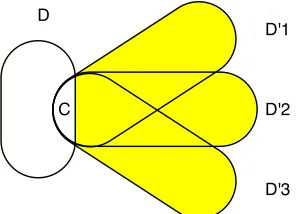
D'1
D'2
D'3 D
[image:8.612.108.257.85.192.2]C
Figure 1: Given setsD01, D02, D30 that intersect setDexactly atCthenMC,Dconsists of the shaded subsets ofD10, D20,and
D30. AssumingCis non-empty,{D10, D02, D30}has a hitting set of size 1 since any vertex inChits all sets. Lemma 3.6 bounds the size of the minimum hitting set of{D01, D20, D03}
that may not include any vertices inC.
(d−1)!kd−1=O(kd−1). To construct the sunflower onC∗, fori = 1, . . . , k+ 1, we pick an edgeDiin the maximum
sunflower with coreCisuch thatDi∩Cj=C∗forj6=iand
Di∩Dj =C∗forj < i. This is possible ifais sufficiently
large.
The sets U and F play a similar role to the sets of the same name in the previous section. For example, if
d= 2, then a large core corresponds to a high degree vertex. However, the setU0has no corresponding notion whend= 2 because a high degree vertex cannot contain another high degree vertex. The following (rather technical) lemma will play a crucial role when dealing with cores that are subsets of other cores inU0or of edges inF. It shows that if a core
Cis contained in a setD, then the set of edges that intersect
DatChas a hitting set that a) does not include vertices inC
and b) has small size assumingsG(C)is small.
LEMMA3.6. For any two sets of verticesC, D, whereC⊆
D, define
MC,D={D0\C|D0 ∈E, D∩D0=C}.
Thenhs(MC,D)≤sG(C)d. See Figure 1 for an example.
Proof. Consider the size of minimum hitting set ofMC,D.
Ifhs(MC,D)> sG(C)d, thenMC,Dhas a matching of size
greater thansG(C). This matching together with the setC
forms a sunflower with coreCand oversG(C)petals, which
contradicts the assumption. Therefore,hs(MC,D)≤sG(C)d
as claimed.
Hitting Set. For the rest of this section we let G0 = (V, E0) ∼ Sampleb,d,r(G) where b = O(k), d is the
cardinality of the hyperedges, andr=O(logk). It will also be convenient to use the notationHS(S)to denote a minimum hitting set of a collection of setsS, i.e.,hs(S) =|HS(S)|.
THEOREM3.2. Suppose hs(G) ≤ k. With probability
1−1/poly(k),hs(G0) = hs(G).
Proof. For each significant coreC there has to be at least
one vertex from the hitting set inC. Since all large cores are significant,hs(G) = hs(U∪F). IfC∈Uhas a subset
C0 such thatsG(C0) > k, then there is at least one vertex
from the hitting set inC0 and this vertex also hitsC. Thus, hs(G) = hs(U0∪F). By Lemma 3.7, the set of significant cores in G0 is a superset ofU0 with high probability. By Lemma 3.8, every edge inF is inG0with high probability.
LEMMA3.7. P[∀C∈U0, sG0(C)> k]≥1−1/poly(k).
Proof. Fix an arbitrary core C ∈ U0. Consider H ∼
Sampleb,d,1 and let c : [n] → [b] be the coloring that defined H. We need to identify k + 1 sets of colors
S1, S2, . . . Sk+1 ⊂ [b]each of size d, such that any set of edges D1, D2, . . . , Dk+1 where Di is Si-colored forms a
sunflower of sizek+ 1on coreC. In order for this to hold, the color sets have to satisfy the following three properties:
1. All edges that areSi-colored containC.
2. There is at least oneSi-colored edge.
3. IfDisSi-colored andD0isSj-colored then(D\C)∩
(D0\C) =∅.
In what follows, we first define a setF ={S1, S2, . . .}that satisfies the above properties. We then argue that|F | ≥k+ 1 with probability at least 1/2. By repeating the process
O(logk)times will ensure that such a family exists with high probability. The lemma follows by taking the union bound over allC∈U0since|U0|=O(kd−1)by Lemma 3.5.
Property 1.We first define a set of verticesAsuch that any edge that does not intersect Amust includeC. Then, for anyS⊂[b]that is disjoint fromc(A), we may infer that all
S-colored edges containC. This follows since ifS=c(D) for some edgeD, thenc(D)∩c(A) =∅which implies that
D∩A=∅, and soC⊆D. Let
A= (HS(G)\C)∪
S
C0⊂CHS(MC0,C)
.
All edges that do not intersectHS(G)\Cmust intersect with
C. But all edges that intersect with only a subset ofC, sayC0, must intersect withHS(MC0,C). HenceAhas the claimed
property. We will say thatCis agood coreifc(C)∩c(A) =∅
Property 2.Next, letPbe a set of petals in a sunflower with coreCthat do not intersect withA. We may choose a set of
|P|=ak− |A|such petals. For eachP ∈ P, define the set:
AP =A∪C∪
S
Q∈P\PQ
.
If C is a good core, let P0 contain all P ∈ P such that
c(P)∩c(AP) =∅and|c(P)|=|P|. IfCis not a good core,
letP0=∅. Then the familyF={c(P∪C)}
P∈P0 satisfies
Properties 1 and 2. Note that no two petals inP0share the same color and hence|F |=|P0|assumingCis a good core.
Property 3.AssumeCis a good core since otherwiseF=∅
and Property 3 is trivially satisified. Let S1, S2 ∈ F and supposeS1 = c(C∪P1)andS2 = c(C∪P2)for some
P1, P2 ∈ P0. Suppose edgesC∪Q1andC∪Q2areS1 -colored andS2-colored respectively. Thenc(Q1) = c(P1) andc(Q2) = c(P2)because|c(C)| =|C|,|c(P1)| = |P1|,
|c(P2)| = |P2|, and all edges have the same cardinality. But c(P1)∩c(P2) = ∅ implies c(Q1)∩c(Q2) = ∅ and soQ1∩Q2=∅as required.
Size of F. We need to show that|P0| ≥ (k+ 1) with probability1/2. Recall thatc:V →[b]is chosen randomly from a family of pairwise independent hash functions and suppose b = 8 max(d|A| +d2, d|A
P|+d2). Note that
b=O(k)since, by appealing to Lemma 3.6,
|A| ≤ |AP| ≤ |A|+|C|+d|P| ≤ hs(G) + X
C0⊂C
hs(MC,C0) +|C|+d|P|
≤ k+ 2ddk+d+dak=O(k).
Then,
P[Cis not a good core]
= P[c(C)∩c(A)=6 ∅or|c(C)| 6=|C|]
≤ (d|A|+d2)/b≤1/8.
For eachP ∈ P, letXP = 1ifP 6∈ P0orCis not a good
core. LetXP = 0otherwise. Then
E hX
XP
i
≤ |P| d|AP|+d2)/b+ 1/8
≤ |P|/4,
and so
P hX
XP ≥ |P|/2
i ≤1/2
by the Markov inequality. Hence,
|P0|=|P| −XXP ≥ |P|/2 =ak/2− |A|/2≥k+ 1
for sufficiently largeawith probability at least1/2.
LEMMA3.8. P[F ⊆E0]≥1−1/poly(k).
Proof. Pick an arbitrary edge D ∈ F. Consider H ∼
Sampleb,d,1and letc: [n]→[b]be the coloring that defined
H. It suffices to show that there is a unique edge that is
c(D)-colored since thenD is necessarily an edge inH. It suffices to show that this is the case with probability at least 1/2because repeating the processO(logk)times will ensure that such a family exists with high probability. The result then follows by taking the union bound over allD∈Fsince
|F|=O(kd)by Lemma 3.5.
LetS=c(D). We first define a setAof vertices such that the only edge that is disjoint fromAisD. It follows that
Dis the uniqueS-colored edge ifS∩c(A) =∅, since every other edge intersectsAand hence must share a color with it. We defineAas follows:
A= (HS(G)\D)∪ S
C⊂DHS(MC,D)
.
NoteDitself is disjoint fromAsince eachHS(MC,D)does
not include vertices from D. If an edge is disjoint from (HS(G)\D)then it must intersectD. Suppose there exists an edgeD0such thatD∩D0 =C 6=D, thenD0intersects HS(MC,D). Hence, the only edge that is disjoint from
A includes the vertices inD and so is equal to D on the assumption that all edges have the same number of vertices. It remains to show thatS∩c(A) =∅with probability at least1/2. Ifb≥2d|A|then we have
P[S∩c(A) =∅]≥1−d|A|/b≥1/2.
Finally, note that b = O(k) since |A| ≤ hs(G) +
P
C⊂Dhs(MC,D) ≤ k+ 2dakd = O(k)by appealing to
Lemma 3.6 and using the fact thatsG(C)≤akfor allC⊂D
sinceD∈F.
A result for hypergraph matching follows along similar lines.
THEOREM3.3. Suppose match(G) ≤ k0 = k/d. With
probability1−1/poly(k),match(G0) = match(G).
Proof. hs(G)≤dk0=k. LetM be the matching.F∩M is
preserved inG0. Consider an edgeD∈M such thatC⊆D
for someC ∈U. Then inG0 we can find (by Lemma 3.7) at leastk+ 1petals in a sunflower with core eitherCitself or someC0 ⊂ C. At mostk of those intersectM \ {D}. Therefore, there is still at least one edge we can pick for the
matching.
4 Approximating Large Matchings
(which they show is optimal). Konrad [36] proves slightly weaker bounds. Bury and Schwiegelshohn [11] present an algorithm for estimating thesizeof the maximum matching in graphs of bounded arboricity. Our second algorithm in this section is similar (the difference is that we can find the edges of an exact matching when it is small whereas they approx-imate the cardinality in this case by guessing and verifying the rank of a related matrix).
4.1 Approximating Matching in Arbitrary Graphs
Intuition and Preliminaries.Given a hash functionc:V →
[b], we say an edgeuvis colorediifc(u) =c(v) =i. If the endpoints have different colors, we say the edge isuncolored. The basic idea behind our algorithm is to repeatedly sample a set of colored edges with distinct colors. Note that a set of colored edges disjoint colors is a matching. We use the edges in this matching to augment the matching already constructed from previous rounds. In this section we require the hash functions to beO(k)-wise independent and, in the context of dynamic data streams, this will increase the update time by a
O(k)factor.
THEOREM4.1. Supposematch(G)≥k. For any1≤α≤ √
kand0< ≤1, with probability1−1/poly(k),
match(G0)≥
1−
2α
·k ,
whereG0∼Sample2k/α,1,rwherer=O(kα−2−2logk).
Note that ifmatch(G)≥10k, = 0.1, andα= 3, then the theorem above implies that we can find a matching of size strictly greater thatkusingO˜(k2)space in the dynamic graph stream model. If match(G) ≤ 10k then if we run the algorithm used for Theorem 3.1, we can find the exact matching usingO˜(k2)space. Hence, we can distinguish between the casematch(G)≤kandmatch(G)> kusing
˜
O(k2)space.
Proof. [Proof of Theorem 4.1] Let H1, . . . , Hr ∼
Sample2k/α,1,1and letG0be the union of these graphs. Con-sider the greedy matchingMrwhereM0=∅and fort≥1,
Mtis the union ofMt−1and additional edges fromHt. We
will show that ifMt−1is small, then we can find many edges inHtthat can be used to augmentMt−1.
Consider Ht and suppose |Mt−1| < 12−α ·k. Let
c : V →[b]be the hash-function used to defineHtwhere
b=2k
α. LetU be the set of colors that are not used to color
the endpoints ofMt−1, i.e.,
U ={c∈[b] : there does not exist a matched vertex
uinMt−1withc(u) =c}. and note that|U| ≥b−2|Mt−1| ≥ αk. For eachc∈U, define the indicator variableXcwhereXc= 1if there exists an edge
uvwithc(u) =c(v) =c. We will findX =P
c∈UXcedges
to add to the matching.
Sincematch(G)≥k, there exists a setk−2|Mt−1|>
k vertex disjoint edges that can be added to Mt−1. Let
p = 2αk and observe that E[Xc] ≥ kp2 − k2
p4 > kp2/2 =·α2
8k.Therefore,E[X]≥( k α)··
α2
8k = α
8 . Since
Xc and Xc0 are negative correlated, P[X ≥E[X]/2] ≥
1 −exp (−Ω (α)) ≥ Ω(). Hence, with each repetition we may increase the size of the matching by at leastα/2 with probabilityΩ(). AfterO(kα−2−2logk)repetitions the matching has size at least 12−α·k.
By applying Theorem 4.1 for allk∈ {1,2,4,8,16, . . .}
and appealing to Theorem 2.1, we establish:
COROLLARY4.1. There exists aO(npolylogn)-space
al-gorithm that returns anO(n1/3)-approximation to the size of
the maximum matching in the dynamic graph stream model.
Proof. For1 ≤ i ≤ logn, letG0i ∼ Sampleb,1,r where
r=O(2iα−2logk)andb= 2i+1/α. These graphs can be generated inO˜(n2α−3)space. For somei,
2i≤match(G)<2i+1
and hencematch(G0i) = Ω(match(G)/α). This result generalizes to the weighted case using the Crouch-Stubbs technique [15]. They showed that if we can find aβ-approximation to the maximumcardinalitymatching amongst all edges of weight greater than(1 +)ifor eachi,
then we can find a2(1 +)β-approximation to the maximum weighted matching.
4.2 Matchings in Planar and Bounded-Arboricity Graphs
In this section, we present an algorithm for estimating the size of the matching in a graph of bounded arboricity. Recall that a graph hasarboricityνif its edges can be partitioned into at mostν forests. In particular, it can be shown that a planar graph has arboricity at most 3. We will make repeated use of the fact that the average degree of every subgraph of a graph with arboricityνis at most2ν.
Our algorithm is based on an insertion-only streaming algorithm due to Esfandiari et al. [21]. They first proved upper and lower bounds on the size of the maximum matching in a graph of arboricityν.
LEMMA4.1. (ESFANDIARI ET AL. [21]) For any graphG
with arboricityν, define a vertex to beheavyif its degree is
at least2ν+ 3and define an edge to beshallowif it is not
incident to a heavy vertex. Then,
max{h, s}
wherehis the number of heavy vertices andsis the number of shallow edges.
To estimatemax{h, s}, Esfandiari et al. sampled a set of verticesZand (a) computed the exact degree of these vertices, then (b) found the set of all edges in the induced subgraph on these vertices. The fraction of heavy vertices inZand shallow edges in the induced graph are then used to estimatehands. By choosing the size ofZappropriately, they showed that the resulting estimate was sufficiently accurate on the assumption thatmax{h, s}is large. In the case wheremax{h, s}is small, the maximum matching is also small and hence a maximal matching could be constructed in small space using a greedy algorithm.
Algorithm for Dynamic Graph Streams. In the dynamic graph stream model, it is not possible to construct a maximal matching. However, we may instead use the algorithm of Theorem 3.1 to find the exact size of the maximum matching. Furthermore we can still recover the induced subgraph on sampled verticesZ via a sparse recovery sketch [25]. This can be done space-efficiently because the number of edges is at most2ν|Z|. Lastly, rather than fixing the size ofZ, we consider sampling each vertex independently with a fixed probability as this simplifies the analysis significantly. The resulting algorithm is as follows:
1. Invoke algorithm of Theorem 3.1 fork= 2n2/5and let
rbe the reported matching size.
2. In parallel, sample vertices with probability p = 8−2n−1/5 and let Z be the set of sampled vertices. Find the degrees of vertices inZ inGand maintain a 2ν|Z|-sparse recovery sketch of the edges in the induced graph onZ. LetsZ be the number of shallow edges
in the induced graph onZand letsZbe the number of
heavy vertices inZ. Returnmax{r, hZ/p, sZ/p2}.
Analysis. Our analysis relies on the following lemma that shows thatmax{hZ/p, sZ/p2}is a1 +approximation for
max{s, h}on the assumption thatmax{s, h} ≥n2/5.
LEMMA4.2. With probability at least4/5,
|max{hZ/p, sZ/p2} −max{s, h}| ≤·max{n2/5, s, h}.
Proof. First we showsZ/p2is a sufficiently good estimate
fors. LetSbe the set of shallow edges inGand letEZ be
the set of edges in the induced graph onZ. For each shallow edgee∈S, define an indicator random variableXewhere
Xe= 1iffe∈EZand note thatsZ =Pe∈SXe. Then,
E[sZ] =sp2
and
V[sZ] =
X
e∈S
X
e0∈S
E[XeXe0]−E[Xe]E[Xe0] .
Note that
X
e0∈S
E[XeXe0]−E[Xe]E[Xe0]
=
p2−p4 ife=e0
p3−p4 ifeande0share exactly one endpoint 0 ifeande0share no endpoints
.
and since there are at most2ν+3edges that share an endpoint with a shallow edge,
V[sZ]≤s(p2−p4+ (2ν+ 3)p3−p4)≤2sp2
on the assumption that (2ν + 3) ≤ 1/p. We then use Chebyshev’s inequality to obtain
P h
|sZ−sp2| ≤p2·max{n2/5, s}
i
≤ 2sp
2
(p2·max{n2/5, s})2 ≤9/10
.
(4.2)
Next we show thathZ/pis a sufficiently good estimate
forh. LetH denote the set ofhheavy vertices inGand define an indicator random variable Yv for eachv ∈ H,
whereYv = 1iffv ∈ Z. Note thathZ = Pv∈HYv and
E[hZ] = hp. Then, by an application of the
Chernoff-Hoeffding bound,
P h
|hZ−hp| ≥pmax{h, n2/5}
i
≤exp(−2pn2/5/3)≤9/10
.
(4.3)
Therefore, it follows from Eq. 4.2 and 4.3 that with probability at least4/5,
|max{hZ/p, sZ/p2} −max{s, h}| ≤·max{n2/5, s, h}.
THEOREM4.2. There exists aO˜(ν−2n4/5logδ−1)-space
dynamic graph stream algorithm that returns a(5ν+ 9)(1 +
)2approximation ofmatch(G)with probability at least1−δ
whereνis the arboricity ofG.
Proof. To argue the approximation factor, first suppose
match(G) ≤ 2n2/5. In this case r = match(G) and max{s, h} ≤(2.5ν+4.5) match(G)by appealing to Lemma 4.1. Hence,
match(G)≤max{r, hZ/p, sZ/p2} ≤(2.5ν+4.5) match(G)
Next suppose match(G) ≥ 2n2/5. In this case, max{s, h} ≥ n2/5 by Lemma 4.1. Therefore, by Lemma 4.2,max{hZ/p, sZ/p2}= (1±) max{s, h}, and so
match(G)
2(1 +) ≤ max{r, hZ/p, sZ/p 2}
≤ (1 +) max{s, h}
To argue the space bound, recall that the algorithm used in Theorem 3.1 requires O˜(n4/5) space. Note that
|Z| ≤2np = ˜O(−2n4/5)with high probability. Hence, to sample the verticesZand maintain a2ν|Z|-sparse recovery data structure requiresO˜(n4/5ν)space.
5 Sampling Kernels for Subgraph Search Problems
We extend our parameterized results to a class of problems where the objective is to search for a subgraphH ofG(V, E) which satisfies some propertyP. In the parameterized setting, we typically search for the largestH which satisfies this property, subject to the promise that the size of any H
satisfying P is at most k. For concreteness, we assume the size is captured by the number of vertices in H, and our objective is to find a maximum cardinality satisfying subgraph. The sampling primitiveSampleb,2,1can be used here whenPis preserved under vertex contraction: ifG0is a vertex contraction ofG, then any subgraphHofG0satisfying
P also satisfiesP forG(with vertices suitably remapped). Here, the vertex contraction of verticesuandvcreates a new vertex whose neighbors areΓ(u)∪Γ(v). Many well-studied problems possess the required structure, including:
—b-matching, finding a maximum cardinality subgraphHof
Gsuch that the degree of each vertex inHis at mostb. Hence, the standard notion of matching in Section 2 is equivalent to 1-matching.
— k-colorable subgraph, finding a subgraph H that isk -colorable. The maximum cardinality 2-colorable subgraph forms a max-cut, and more generally the maximum cardinal-ityk-colorable subgraph is a maxk-cut.
— other maximum subgraph problems, such as finding the largest subgraph that is a forest, has at least c connected components, or is a collection of vertex disjoint paths.
THEOREM5.1. LetP be a graph property preserved under vertex contraction. Suppose that the number of vertices in
some optimum solution opt(G) is at most k. Let G0 ∼
Sample4k2,2,1(G). With constant probability, we can compute
a solutionH forPfromG0that achieves|H|=|opt(G)|.
Proof. We construct acontracted graphG00fromG0based on
the color classes used in theSampleoperator: we contract all vertices that are assigned the same color by the hash function
c(). Fix an optimum solutionopt(G)with at mostkvertices. Lemma 2.1 shows that for b = 4k2, all vertices involved in opt(G) are hashed into distinct color values. Hence, the subgraph opt(G) is a subgraph ofG00: for any edge
e = (u, v) ∈ opt(G), the edge itself was sampled from the data structure, or else a different edge with the same color values was sampled, and so can be used interchangeably in
G00. Hence, (the remapped form of)opt(G)persists inG00. By the vertex contraction property ofP, this means that a
maximum cardinality solution forP inG00 is a maximum cardinality solution inG.
Note that for this application of the subgraph sampling primitive, it suffices to implement the sampling data structure with a counter for each pair of colors: any non-zero count
corresponds to an edge inG00.
Note that the generality of the result comes at the cost of increasing the number of colors, and hence the space of the stream algorithms. To generalize the result to the weighted case (e.g., where the objective is to find the subgraph satisfying P with the greatest total weight), we take the approach used in Section 3.1. We perform the sampling in parallel for each distinct weight value, and then round each edge weight to the closest power of(1 +)to reduce the number of weight classes toO(−1logW), with a loss factor of(1 +).
6 Lower Bounds
6.1 Matching and Hitting Set Lower Bounds
The following theorem establishes that the space-use of our matching, vertex cover, hitting set, and hyper matching algorithms is optimal up to logarithmic factors.
THEOREM6.1. Any (randomized) parameterized
stream-ing algorithm for the minimum d-hitting set or maximum
(hyper)matching problem with parameterkrequiresΩ(kd)
space.
Proof. We reduce from the MEMBERSHIPproblem in
com-munication complexity:
MEMBERSHIP
Input: Alice has a setX ⊆[n], and Bob has an element
1≤x≤n.
Question: Bob wants to check whetherx∈X.
There is a lower bound ofΩ(n)bits of communication from Alice to Bob, even allowing randomization [2].
LetS =s1s2...snbe the characteristic string ofX, i.e.
a binary string such thatsi= 1iffi∈X. Letk= d √
n. Fix a canonical mappingh: [n]→[k]d. This way we can view
annbit string as an adjacency matrix of ad-partite graph. Construct the following graph G with dvertex partitions
V1, V2, ..., Vd:
• Each partitionVihasdkvertices: for eachj∈[k]create
verticesv∗i,j,v1
i,j,vi,j2 ,...,v d−1 i,j . • Alice inserts a hyperedge(v∗1,j
1, v
∗ 2,j2, ..., v
∗
d,jd)iff the
corresponding bit in the stringSis 1, i.e.,sa= 1where
h(a) = (j1, j2, ..., jd).
• Let h(x) = (J1, J2, ..., Jd). Bob inserts edge
Alice runs the (assumed) hitting set algorithm on the edges she is inserting using spacef(k). Then she sends the memory contents of the algorithm to Bob, who finishes running the algorithm on his edges.
The minimum hitting set should include vertices vi,j∗
such thatj 6= Ji. If edge(v1∗,J1, v
∗ 2,J2, ..., v
∗
d,Jd)is in the
graph, we also need to include one of its vertices. Therefore,
x∈X ⇐⇒ sx= 1 ⇐⇒ (v∗1,J
1, v
∗ 2,J2, ..., v
∗
d,Jd)is inG ⇐⇒ hs(G) =dk−d+ 1.
On the other hand,
x6∈X ⇐⇒ sx= 0
⇐⇒ (v1∗,J1, v2∗,J2, ..., v∗d,Jd)is not inG
⇐⇒ hs(G) =dk−d .
Alice only sends f(k) bits to Bob. Therefore, f(k) = Ω(n) = Ω(kd).
For the lower bound on matching we use the same construction. For each vertexv∗
i,jsuch thatj6=Jimaximum
matching should include(vi,j∗ , vi,j1 , vi,j2 , ..., vi,jd−1). If edge (v∗
1,J1, v
∗ 2,J2, ..., v
∗
d,Jd)is in the graph, we include it in the
matching as well. Therefore,
x∈X ⇐⇒ sx= 1 ⇐⇒ (v∗1,J
1, v
∗ 2,J2, ..., v
∗
d,Jd)is inG ⇐⇒ match(G) =dk−d+ 1.
And
x6∈X ⇐⇒ sx= 0
⇐⇒ (v1∗,J1, v2∗,J2, ..., v∗d,Jd)is not inG
⇐⇒ match(G) =dk−d .
6.2 Lower Bounds for Problems considered by Fafianie and Kratsch [22]
Comparison with Lower Bounds for Streaming Kernels: Fafianie and Kratsch [22] introduced the notion of kerneliza-tion in the streaming setting as follows:
DEFINITION6.1. A 1-pass streaming kernelization
algo-rithm receives an input(x, k)and returns a kernel, with the
restriction that the space usage of the algorithm is bounded
byp(k)·log|x|for some polynomialp.
Fafianie and Kratsch [22] gave deterministic lower bounds for several parameterized problems. In particular, they showed that:
• Any 1-pass kernel for EDGE DOMINATING SET(k) requiresΩ(m)bits, wheremis the number of edges. However, there is a 2-pass kernel which usesO(k3· logn)bits of local memory andO(k2)time in each step and returns an equivalent instance of sizeO(k3·logk).
• The lower bound ofΩ(m)bits for any 1-pass kernel also holds for several other problems such as CLUS -TEREDITING(k), CLUSTERDELETION(k), CLUSTER VERTEX DELETION(k), COGRAPH VERTEX DELE -TION(k), MINIMUM FILL-IN(k), EDGE BIPARTIZA -TION(k), FEEDBACK VERTEXSET(k), ODD CYCLE TRANSVERSAL(k), TRIANGLEEDGEDELETION(k), TRIANGLEVERTEXDELETION(k), TRIANGLEPACK -ING(k),s-STARPACKING(k), BIPARTITECOLORFUL NEIGHBORHOOD(k).
• Anyt-pass kernel for CLUSTEREDITING(k)and MINI -MUMFILL-IN(k)requiresΩ(n/t)space.
In this section, we giveΩ(n)randomized lower bounds for the space complexity of all the problems considered by Fafianie and Kratsch. In addition, we also consider some other problems such as PATH(k)which were not considered by Fafianie and Kratsch. A simple observation shows that any lower bound for parameterized streaming kernels also transfers for the parameterized streaming algorithms. Thus the results of Fafiane and Kratsch [22] also give lower bounds for the parameterized streaming algorithms for these problems. However, our lower bounds have the following advantage over the results of [22]:
• All our lower bounds also hold forrandomized
algo-rithms, whereas the kernel lower bounds were for
deter-ministic algorithms.
• With the exception of EDGEDOMINATINGSET(k), all our lower bounds also hold for anyconstant number of
passes.
6.2.1 Lower Bound for EDGEDOMINATINGSET
We now show a lower bound for the EDGEDOMINATING SET(k)problem.
DEFINITION6.2. Given a graphG= (V, E)we say that a
set of edgesX⊆Eis an edge dominating set if every edge
inE\Xis incident on some edge ofX.
EDGEDOMINATINGSET(k) Parameter:k
Input: An undirected graphsGand an integerk
Question: Does there exist an edge dominating setX ⊆E
of size at mostk?
THEOREM6.2. For theEDGEDOMINATINGSET(k)
prob-lem, any (randomized) streaming algorithm needs Ω(n)
Proof. Given an instance of MEMBERSHIP, we create a graph
Gonn+ 2vertices as follows. For eachi∈[n]we create a vertexvi. Also add two special verticesaandb. For every
y∈X, add the edge(a, y). Finally add the edge(b, x). Now we will show thatGhas an edge dominating set of size 1 iff MEMBERSHIPanswers YES. In the first direction suppose thatGhas an edge dominating set of size 1. Then it must be the case thatx∈X: otherwise for a minimum edge dominating set we need one extra edge to dominate the star incident ona, in addition to the edge(b, x)dominating itself. Hence MEMBERSHIP answers YES. In reverse direction, suppose that MEMBERSHIP answers YES. Then the edge (a, x)is clearly an edge dominating set of size 1.
Therefore, any (randomized) streaming algorithm that can determine whether a graph has an edge dominating set of size at mostk = 1gives a communication protocol for MEMBERSHIP, and hence requiresΩ(n)space.
6.2.2 Lower Bound forG-FREEDELETION
DEFINITION6.3. Let Gbe a set of graphs such that each
graph inGis connected. We say thatGisbadif there is graph
H ∈ Gsuch that
• H is a minimal element ofG under the operation of
taking subgraphs, i.e., no proper subgraph ofHis inG
• Hhas at least two distinct edges
Note thatG={P2}is notbad(whereP2is the path on two vertices) since the only minimal graph inGisP2which does not have two edges. On the other hand, the class of graphsG ={P3, P4, P5, . . .}isbadsinceP3is a minimal graph (under operation of taking subgraphs) ofG andP3 contains two edges.
For any bad set of graphsG, we now show a lower bound for the following general problem:
G-FREEDELETION(k) Parameter:k
Input: A bad set of graphsG, an undirected graphG =
(V, E)and an integerk
Question: Does there exist a setX ⊆V such thatG\X
contains no graph fromG?
We reduce from the DISJOINTNESSproblem in commu-nication complexity.
DISJOINTNESS
Input: Alice has a stringx∈ {0,1}ngiven byx
1x2. . . xn.
Bob has a stringy∈ {0,1}ngiven byy
1y2. . . yn.
Question: Bob wants to check if ∃ i ∈ [n] such that
xi=yi= 1.
There is a lower bound ofΩ(n/p)bits of communication between Alice and Bob, allowingp-rounds and randomiza-tion [39].
THEOREM6.3. For abadset of graphsG, anyp-pass
(ran-domized) streaming algorithm for the G-FREEDELETION
problem needsΩ(n/p)space .
Proof. SinceGis abadset of graphs, there is a minimal graph
H ∈ G which has at least two distinct edges, saye1ande2. LetH0:=H\{e
1, e2}. Given an instance of DISJOINTNESS, we create a graphGwhich consists ofndisjoint copies say
G1, G2, . . . , GnofH0. For eachi∈[n], to the copyGi of
H0we add the edgee1iffxi= 1and the edgee2iffyi= 1.
We now show that the resulting graphGcontains a copy of
H if and only if it is a YES instance of DISJOINTNESS. Suppose that it is a YES instance of DISJOINTNESS. So there is aj ∈ [n]such thatxj = 1 = yj. Therefore, to
the copyGj ofH0we would have added the edgese1and
e2which would produce an instance ofH. SoGcontains a copy ofH. In other direction, suppose thatGcontains a copy ofH. Note that since we addndisjoint copies ofH0
and add at most two edges (e1ande2) to each copy, it follows that each connected component ofGis in fact a subgraph of
H =H0∪(e1+e2). SinceHis connected andGcontains a copy ofH, some connected component ofGmust exactly be the graphH, i.e, to some copyGiofH0we must have added
both the edgese1ande2. This impliesxi= 1 =yi, and so
DISJOINTNESSanswers YES.
Since each connected component of Gis a subgraph ofH, the minimality ofH implies thatGcontains a graph fromGiffGcontains a copy of H, which in turn is true iff DISJOINTNESS answers YES. Therefore, any p-pass (randomized) streaming algorithm that can determine whether a graph isG-free (i.e., answers the question withk= 0) gives a communication protocol for DISJOINTNESS, and hence
requiresΩ(n/p)space.
This implies lower bounds for the following set of problems:
THEOREM6.4. For each of the following problems,
any p-pass (randomized) algorithm requires Ω(n/p)
space: FEEDBACK VERTEX SET(k), ODD CYCLE
TRANSVERSAL(k),EVENCYCLETRANSVERSAL(k)and
TRIANGLEDELETION(k).
Proof. We first define the problems below:
FEEDBACKVERTEXSET(k) Parameter:k
Input: An undirected graphG= (V, E)and an integerk
Question: Does there exist a setX ⊆V of size at mostk
such thatG\X has no cycles?
ODDCYCLETRANSVERSAL(k) Parameter:k
Input: An undirected graphG= (V, E)and an integerk
Question: Does there exist a setX ⊆V of size at mostk
EVENCYCLETRANSVERSAL(k) Parameter:k
Input: An undirected graphG= (V, E)and an integerk
Question: Does there exist a setX⊆V of size at mostk
such thatG\X has no even cycles?
TRIANGLEDELETION(k) Parameter:k
Input: An undirected graphG= (V, E)and an integerk
Question: Does there exist a setX⊆V of size at mostk
such thatG\X has no triangles?
Now we show how each of these problems can be viewed as aG-FREEDELETIONproblem for an appropriate choice ofbadG.
• FEEDBACK VERTEX SET(k): Take G =
{C3, C4, C5, . . .}andH =C3
• ODD CYCLE TRANSVERSAL(k): Take G =
{C3, C5, C7, . . .}andH =C3
• EVEN CYCLE TRANSVERSAL(k): Take G =
{C4, C6, C8, . . .}andH =C4
• TRIANGLEDELETION(k): TakeG ={C3}andH =
C3
We verify the conditions for FEEDBACK VERTEXSET(k); the proofs for other problems are similar. Note that the choice ofG={C3, C4, C5, . . .}andH =C3implies thatGisbad since each graph inGis connected, the graphH belongs toG, has at least two distinct edges and is a minimal element ofG
(under operation of taking subgraphs). Finally, finding a set
Xsuch that the graphG\X isG-free implies that it has no cycles, i.e.,X is a feedback vertex set forG.
It is easy to see that the same proofs also work for the edge deletion versions of the ODDCYCLETRANSVER -SAL(k), EVENCYCLETRANSVERSAL(k)and the TRIAN -GLEDELETION(k)problems.
6.2.3 G-EDITING
DEFINITION6.4. We say that a set of graphsG isgoodif
there is graphH ∈ Gsuch that
• H is a minimal element ofG under the operation of
taking subgraphs, i.e., no proper subgraph ofHis inG
• His connected and has at least two distinct edges
Definition 6.4 looks very similar to Definition 6.3: however there is a subtle difference. Each graph in abad
set of graphs must be connected while only a minimal graph in agood set of graphs is required to be connected. This difference is used crucially in the proofs of Theorem 6.3 and Theorem 6.5.
For anygood set of graphsG, we now show a lower bound for the following general problem:
G-EDITING(k) Parameter:k
Input: A graph classG, an undirected graphG= (V, E)
and an integerk
Question: Does there exist a setXofkedges such that
(V, E∪X)contains a graph fromG?
THEOREM6.5. For a good set of graphs G, any p-pass
(randomized) streaming algorithm for the G-EDITING(k)
problem needsΩ(n/p)space.
Proof. We reduce from the DISJOINTNESSproblem in
com-munication complexity. Since G is agood set of graphs, there is a minimal graphH ∈ G such thatH is connected and has at least two distinct edges, say e1 and e2. Let
H0 :=H \ {e1, e2}. Given an instance of DISJOINTNESS, we create a graphGwhich consists ofndisjoint copies say
G1, G2, . . . , GnofH0. By minimality ofH, it follows that
H0∈ G/ . For eachi∈[n]we add toGithe edgee1iffxi = 1
and the edgee2iffyi= 1. Let the resulting graph beG.
We now show thatGcontains a copy ofH if and only if DISJOINTNESS answers YES. Suppose thatG contains a copy ofH. Note that since we addndisjoint copies of
H0 and add at most two edges (e1 ande2) to each copy, it follows that each connected component of Gis in fact a subgraph ofH = H0 ∪(e1+e2). Since H is connected andGcontains a copy ofH, some connected component of
Gmust exactly be the graphH, i.e, to some copyGiofH0
we must have added both the edgese1ande2. This implies
xi = 1 = yi, and so DISJOINTNESSanswers YES. Now
suppose that DISJOINTNESSanswers YES, i.e., there exists
j∈[n]such thatxj= 1 =yj. Therefore, to the copyGjof
H0we would have added the edgese1ande2which would complete it intoH. SoGcontains a copy ofH.
Otherwise, due to minimality ofH, the graphGdoes not contain any graph from G. Therefore, any p-pass (randomized) streaming algorithm that can determine whether a graph G contains a graph from G (i.e., answers the question withk = 0) gives a communication protocol for DISJOINTNESS, and hence requiresΩ(n/p)space.
This implies lower bounds for the following set of problems:
THEOREM6.6. For each of the following problems, anyp
-pass (randomized) algorithm requiresΩ(n/p)space: TRI
-ANGLEPACKING(k),s-STARPACKING(k)andPATH(k).
Proof. We first define the problems below:
TRIANGLEPACKING(k) Parameter:k
Input: An undirected graphG= (V, E)and an integerk
Question: Do there exist at leastkvertex disjoint triangles